Dynamical behavior in $f(T,T_{G})$ cosmology

Abstract

The $f(T,T_{G})$ class of gravitational modification, based on the quadratic torsion scalar $T$, as well as on the new quartic torsion scalar $T_{G}$ which is the teleparallel equivalent of the Gauss-Bonnet term, is a novel theory, different from both $f(T)$ and $f(R,G)$ ones. We perform a detailed dynamical analysis of a spatially flat universe governed by the simplest non-trivial model of $f(T,T_{G})$ gravity which does not introduce a new mass scale. We find that the universe can result in dark-energy dominated, quintessence-like, cosmological-constant-like or phantom-like solutions, according to the parameter choices. Additionally, it may result to a dark energy - dark matter scaling solution, and thus it can alleviate the coincidence problem. Finally, the analysis “at infinity” reveals that the universe may exhibit future, past, or intermediate singularities depending on the parameters.

1 Introduction

Since the discovery of the universe late-times acceleration, a large amount of research has been devoted to its explanation. In principle, one can follow two main directions to achieve this. The first way is to modify the content of the universe introducing the dark energy concept, with its simpler candidates being a canonical scalar field, a phantom field or the combination of both fields in a unified model dubbed quintom (for reviews on dark energy see [1, 2] and references therein). The second direction that one can follow is to modify the gravitational sector itself (for a review see [3] and references therein), acquiring a modified cosmological dynamics. However, note that apart from the interpretation, one can transform from one approach to the other, since the crucial issue is just the number of degrees of freedom beyond General Relativity and standard model particles (see [4] for a review on such a unified point of view). Finally, note that the above scenarios, apart from late-times implications, can be also used for the description of the inflationary stage [5].

In the majority of modified gravitational theories, one suitably extends the curvature-based Einstein-Hilbert action of General Relativity. However, an interesting class of gravitational modification arises when one modifies the action of the equivalent formulation of General Relativity based on torsion. In particular, it is known that Einstein himself constructed the so-called “Teleparallel Equivalent of General Relativity” (TEGR) [6, 7, 8, 9] using the curvature-less Weitzenböck connection instead of the torsion-less Levi-Civita one. The corresponding Lagrangian, namely the torsion scalar $T$, is constructed by contractions of the torsion tensor, in a similar way that the usual Einstein-Hilbert Lagrangian $R$ is constructed by contractions of the curvature (Riemann) tensor. Thus, inspired by the $f(R)$ modifications of the Einstein-Hilbert Lagrangian [10, 11], one can construct the $f(T)$ modified gravity by extending $T$ to an arbitrary function [12, 13, 14]. Note that although TEGR coincides with General Relativity at the level of equations, $f(T)$ does not coincide with $f(R)$, that is they represent different modification classes. Thus, the cosmological implications of $f(T)$ gravity are new and interesting [14, 15, 16, 17, 19, 20, 18, 21, 22, 23, 24, 25, 26, 27, 28, 29, 30, 31, 32, 33, 34, 35, 36, 37, 38, 39, 40, 41, 42, 43].

However, in curvature gravity, apart from the simple $f(R)$ modification one can construct more complicated extensions using higher-curvature corrections such as the Gauss-Bonnet term $G$ [44, 45, 46] or functions of it [47, 48], Lovelock combinations [49, 50, 51], and Weyl combinations [52, 53, 54]. Inspired by these, in the recent work [55], the $f(T,T_{G})$ gravitational modification was constructed, which is based on the old quadratic torsion scalar $T$, as well as on the new quartic torsion scalar $T_{G}$ that is the teleparallel equivalent of the Gauss-Bonnet term. Obviously, $f(T,T_{G})$ theories cannot arise from the $f(T)$ ones, and additionally they are different from $f(R,G)$ class of curvature modified gravity. Thus, $f(T,T_{G})$ is a novel class of gravitational modification.

The cosmological applications of $f(T,T_{G})$ gravity proves to be very interesting [55]. Therefore, it is both interesting and necessary to perform a dynamical analysis, examining in a systematic way the allowed cosmological behaviors, focusing on the late-times stable solutions. The phase-space and stability analysis is a very powerful tool, since it reveals the global features of a given cosmological scenario, independently of the initial conditions and the specific evolution of the universe. In the present investigation we perform such a detailed phase-space analysis, and we extract the late-times, asymptotic solutions, calculating also the corresponding observable quantities, such as the deceleration parameter, the effective dark energy equation-of-state parameter, and the various density parameters.

The plan of the work is the following: In section 2 we briefly review the scenario of $f(T,T_{G})$ gravity and in section 3 we present its application in cosmology. In section 4 we perform the detailed dynamical analysis for the simplest non-trivial model of $f(T,T_{G})$ gravity. In section 5 we discuss the cosmological implications and the physical behavior of the scenario. Finally, in section 6 we summarize our results.

2 $f(T,T_{G})$ gravity

In this section we briefly review the $f(T,T_{G})$ gravitational modification following [55]. In the whole manuscript we use the following notation: Greek indices run over the coordinate space-time, while Latin indices run over its tangent space.

In this framework the dynamical variable is the vierbein field $e_{a}(x^{\mu})$. In terms of coordinates, it can be expressed in components as $e_{a}=e^{\,\,\,\mu}_{a}\partial_{\mu}$, while the dual vierbein is defined as $e^{a}=e^{a}_{\,\,\,\mu}dx^{\mu}$. Concerning the other field, that is the connection 1-forms $\omega^{a}_{\,\,\,b}(x^{\mu})$ which defines the parallel transportation, one uses the Weitzenböck one, which in all coordinate frames is defined as

$$\omega_{\,\,\,\mu\nu}^{\lambda}=e_{a}^{\,\,\,\lambda}e^{a}_{\,\,\,\mu,\nu}.$$ (2.1)

Due to its inhomogeneous transformation law it has tangent-space components $\omega_{\,\,\,bc}^{a}=0$, assuring the property of vanishing non-metricity. Additionally, for an orthonormal vierbein the metric tensor is given by the relation

$$g_{\mu\nu}=\eta_{ab}\,e^{a}_{\,\,\,\mu}\,e^{b}_{\,\,\,\nu},$$ (2.2)

where $\eta_{ab}=\text{diag}(-1,1,1,1)$ and indices $a,b,...$ are raised/lowered with $\eta_{ab}$.

One can now define the torsion tensor as

$$T^{\lambda}_{\,\,\,\mu\nu}=e_{a}^{\,\,\,\lambda}\left(\partial_{\nu}e^{a}_{\,\,\,\mu}-\partial_{\mu}e^{a}_{\,\,\,\nu}\right),$$ (2.3)

while the Riemann tensor is zero by construction, due to the teleparallelism condition which is imposed with the use of the Weitzenböck connection. Moreover, the contorsion tensor, which equals the difference between the Weitzenböck and Levi-Civita connections, is defined as

$$\mathcal{K}^{\mu\nu}_{\>\>\>\>\rho}=-\frac{1}{2}\Big{(}T^{\mu\nu}_{\>\>\>\>\rho}-T^{\nu\mu}_{\>\>\>\>\>\rho}-T_{\rho}^{\>\>\mu\nu}\Big{)}.$$ (2.4)

Since in this formulation all the information concerning the gravitational field is included in the torsion tensor $T^{\lambda}_{\,\,\,\mu\nu}$, one can use it in order to construct torsion invariants. The simplest invariants that one can build are quadratic in the torsion tensor. In particular, the combination

$$T = \frac{1}{4}T^{\mu\nu\lambda}T_{\mu\nu\lambda}+\frac{1}{2}T^{\mu\nu\lambda}T_{\lambda\nu\mu}-T_{\nu}^{\,\,\,\nu\mu}T^{\lambda}_{\,\,\,\lambda\mu},$$ (2.5)

which can in general be defined in an arbitrary dimension $D$, is the “torsion scalar”, and if it is used as a Lagrangian and be varied in terms of the vierbein it gives rise to the Einstein field equations. That is why the gravitational theory characterized by the action

$$S=-\frac{1}{2\kappa^{2}}\int d^{4}x\,e\,T\,,$$ (2.6)

with $e=\det{(e^{a}_{\,\,\,\mu})}=\sqrt{|g|}$ and $\kappa^{2}\equiv 8\pi G$ the gravitational constant, is called Teleparallel Equivalent of General Relativity. In these lines, one can be based on $T$ in order to construct modified gravitational theories extending the TEGR action to [14, 15, 16, 17, 19, 20, 18, 21, 22, 23, 24, 25, 26, 27, 28, 29, 30, 31, 32, 33, 34, 35, 36, 37, 38, 39, 40, 41, 42, 43]

$$S=\frac{1}{2\kappa^{2}}\int d^{4}x\,e\,f(T)\,.$$ (2.7)

We stress here that although the field equations of TEGR are identical with those of General Relativity, $f(T)$ modification gives rise to different equations than $f(R)$ modification.

However, one can use the torsion tensor in order to construct higher-order torsion invariants, in a similar way that one uses the Riemann tensor in order to construct higher-order curvature invariants. In particular, in [55] the invariant

$$T_{G}=\left(\mathcal{K}^{\kappa}_{\,\,\,\varphi\pi}\mathcal{K}^{\varphi\lambda}_{\,\,\,\,\,\,\,\rho}\mathcal{K}^{\mu}_{\,\,\,\,\chi\sigma}\mathcal{K}^{\chi\nu}_{\,\,\,\,\,\,\,\tau}-2\mathcal{K}^{\kappa\!\lambda}_{\,\,\,\,\,\,\pi}\mathcal{K}^{\mu}_{\,\,\,\varphi\rho}\mathcal{K}^{\varphi}_{\,\,\,\chi\sigma}\mathcal{K}^{\chi\nu}_{\,\,\,\,\,\,\tau}\right.$$

$$\left.\ \ \ \ \ \ \ \ \ \ \ +2\mathcal{K}^{\kappa\!\lambda}_{\,\,\,\,\,\,\pi}\mathcal{K}^{\mu}_{\,\,\,\,\varphi\rho}\mathcal{K}^{\varphi\nu}_{\,\,\,\,\,\,\chi}\mathcal{K}^{\chi}_{\,\,\,\,\sigma\tau}+2\mathcal{K}^{\kappa\!\lambda}_{\,\,\,\,\,\,\pi}\mathcal{K}^{\mu}_{\,\,\,\,\varphi\rho}\mathcal{K}^{\varphi\nu}_{\,\,\,\,\,\,\,\sigma,\tau}\right)\delta^{\pi\rho\sigma\tau}_{\kappa\lambda\mu\nu}$$ (2.8)

was constructed in an arbitrary dimension $D$, where the generalized $\delta^{\pi\rho\sigma\tau}_{\kappa\lambda\mu\nu}$ is the determinant of the Kronecker deltas. This invariant is just the Teleparallel Equivalent of the Gauss-Bonnet combination $G=R^{2}-4R_{\mu\nu}R^{\mu\nu}+R_{\mu\nu\kappa\lambda}R^{\mu\nu\kappa\lambda}$, and in four dimensions it reduces to a topological term. Thus, inspired by the $f(G)$ extensions of General Relativity [47, 48], one can consider general functions $f(T_{G})$ in the action too.

Taking the above into account, one can propose a new class of gravitational modifications as [55]

$$S=\frac{1}{2\kappa^{2}}\!\int d^{4}x\,e\,f(T,T_{G})\,,$$ (2.9)

which is also valid in higher dimensions. Since $T_{G}$ is quartic in the torsion tensor, $f(T,T_{G})$ gravity is more general than the $f(T)$ class. Additionally, $f(T,T_{G})$ gravity is obviously different from $f(R,G)$ one [47, 48, 56, 57, 58]. Note that the usual Einstein-Gauss-Bonnet theory for $D>4$ arises in the special case $f(T,T_{G})=-T+\alpha T_{G}$ (with $\alpha$ the Gauss-Bonnet coupling), while TEGR (that is GR) is obtained for $f(T,T_{G})=-T$.

3 $f(T,T_{G})$ cosmology

In order to investigate the cosmological implication of the above action (2.9), we consider a spatially flat cosmological ansatz

$$ds^{2}=-dt^{2}+a^{2}(t)\delta_{\hat{i}\hat{j}}dx^{\hat{i}}dx^{\hat{j}}\,,$$ (3.1)

where $a(t)$ is the scale factor. This metric arises from the diagonal vierbein

$$e^{a}_{\,\,\,\mu}=\text{diag}(1,a(t),a(t),a(t))$$ (3.2)

through (2.2), while the dual vierbein is $e_{a}^{\,\,\,\mu}=\text{diag}(1,a^{-1}(t),a^{-1}(t),a^{-1}(t))$, and its determinant $e=a(t)^{3}$. Thus, inserting the vierbein (3.2) into relations (2.5) and (2.8), we find

$$T=6H^{2}$$ (3.3)

$$T_{G}=24H^{2}\big{(}\dot{H}+H^{2}\big{)},$$ (3.4)

where $H=\frac{\dot{a}}{a}$ is the Hubble parameter and dots denote differentiation with respect to $t$.

Finally, in order to acquire a realistic cosmology we additionally consider a matter action $S_{m}$, corresponding to an energy-momentum tensor $\Theta^{\mu\nu}$, focusing on the case of a perfect fluid of energy density $\rho_{m}$ and pressure $p_{m}$.

As it was showed in [55], variation of the total action $S+S_{m}$ gives in the case of FRW geometry the following Friedmann equations

$$f-12H^{2}f_{T}-T_{G}f_{T_{G}}+24H^{3}\dot{f_{T_{G}}}=2\kappa^{2}\rho_{m}$$ (3.5)

$$f-4\big{(}3H^{2}+\dot{H}\big{)}f_{T}-4H\dot{f_{T}}-T_{G}f_{T_{G}}+\frac{2}{3H}T_{G}\dot{f_{T_{G}}}+8H^{2}\ddot{f_{T_{G}}}=-2\kappa^{2}p_{m}\,,$$ (3.6)

where $\dot{f_{T}}=f_{TT}\dot{T}+f_{TT_{G}}\dot{T}_{G}$, $\dot{f_{T_{G}}}=f_{TT_{G}}\dot{T}+f_{T_{G}T_{G}}\dot{T}_{G}$, $\ddot{f_{T_{G}}}=f_{TTT_{G}}\dot{T}^{2}+2f_{TT_{G}T_{G}}\dot{T}\dot{T}_{G}+f_{T_{G}T_{G}T_{G}}\dot{T}_{G}^{\,\,2}+f_{TT_{G}}\ddot{T}+f_{T_{G}T_{G}}\ddot{T}_{G}$, with $f_{TT}$, $f_{TT_{G}}$,… denoting multiple partial differentiations of $f$ with respect to $T$, $T_{G}$. Here, the involved time-derivatives of $\dot{T}$, $\ddot{T}$, $\dot{T}_{G}$, $\ddot{T}_{G}$ are straightforwardly obtained using (3.3), (3.4).

Therefore, we can rewrite the Friedmann equations (3.5) and (3.6) in the usual form

$$H^{2} = \frac{\kappa^{2}}{3}\left(\rho_{m}+\rho_{DE}\right)$$ (3.7)

$$\dot{H} = -\frac{\kappa^{2}}{2}\left(\rho_{m}+p_{m}+\rho_{DE}+p_{DE}\right),$$ (3.8)

defining the energy density and pressure of the effective dark energy sector as

$$\rho_{DE}\equiv\frac{1}{2\kappa^{2}}\left(6H^{2}-f+12H^{2}f_{T}+T_{G}f_{T_{G}}-24H^{3}\dot{f_{T_{G}}}\right)$$ (3.9)

$$p_{DE}\equiv\frac{1}{2\kappa^{2}}\left[\!-2(2\dot{H}\!+\!3H^{2})+f\!-\!4\big{(}\dot{H}\!+\!3H^{2}\big{)}f_{T}-4H\dot{f_{T}}-T_{G}f_{T_{G}}+\frac{2}{3H}T_{G}\dot{f_{T_{G}}}+8H^{2}\ddot{f_{T_{G}}}\right]\!.$$ (3.10)

The standard matter $\rho_{m}$ is conserved independently, i.e. $\dot{\rho}_{m}+3H(\rho_{m}+p_{m})=0$. One can easily verify that the dark energy density and pressure satisfy the usual evolution equation

$$\dot{\rho}_{DE}+3H(\rho_{DE}+p_{DE})=0,$$ (3.11)

and we can also define the dark energy equation-of-state parameter as usual

$$w_{DE}\equiv\frac{p_{DE}}{\rho_{DE}}.$$ (3.12)

4 Dynamical analysis

In order to perform the stability analysis of a given cosmological scenario, one first transforms it to its autonomous form $\textbf{X}^{\prime}=\textbf{f(X)}$ [59, 60, 61, 62, 63, 64, 65], where X are some auxiliary variables presented as a column vector and primes denote derivatives with respect to $N=\ln a$. Then, one extracts the critical points $\bf{X_{c}}$ by imposing the condition $\bf{X}^{\prime}=0$, and in order to determine their stability properties one expands around them with U the column vector of the perturbations of the variables. Therefore, for each critical point the perturbation equations are expanded to first order as $\textbf{U}^{\prime}={\bf{Q}}\cdot\textbf{U}$, with the matrix ${\bf{Q}}$ containing the coefficients of the perturbation equations. The eigenvalues of ${\bf{Q}}$ determine the type and stability of the specific critical point.

In order to perform the above analysis, we need to specify the $f(T,T_{G})$ form. In usual $f(T)$ gravity one starts adding corrections of $T$-powers. However, in the scenario at hand, since $T_{G}$ contains quartic torsion terms it is of the same order with $T^{2}$. Therefore, $T$ and $\sqrt{T^{2}+\alpha_{2}T_{G}}$ are of the same order, and thus, one should use both in a modified theory. Hence, the simplest non-trivial model, which does not introduce a new mass scale into the problem and differs from General Relativity, is the one based on

$$f(T,T_{G})=-T+\alpha_{1}\sqrt{T^{2}+\alpha_{2}T_{G}}\,.$$ (4.1)

The couplings $\alpha_{1},\alpha_{2}$ are dimensionless and the model is expected to play an important role at late times. Indeed, this model, although simple, can lead to interesting cosmological behavior, revealing the advantages, the capabilities, and the new features of $f(T,T_{G})$ cosmology. We mention here that when $\alpha_{2}=0$ this scenario reduces to TEGR, that is to General Relativity, with just a rescaled Newton’s constant, whose dynamical analysis has been performed in detail in the literature [61, 62, 63]. Thus, in the following we restrict our analysis to the case $\alpha_{2}\neq 0$.

In this case, the cosmological equations are the Friedmann equations (3.7), (3.8), with the effective dark energy density and pressure (3.9) and (3.10) becoming

$$\!\!\!\!\!\!\!\!\!\!\!\!\!\!\!\!\!\!\!\!\!\!\!\!\!\!\!\!\!\!\!\!\!\!\!\!\!\!\!\!\!\!\!\!\!\!\!\!\!\!\!\!\!\!\!\!\!\!\!\!\!\!\!\!\!\!\!\!\!\!\!\!\!\!\!\!\!\kappa^{2}\rho_{DE}=\frac{\sqrt{3}\alpha_{1}H^{2}\left\{\alpha_{2}^{2}\ddot{H}+9\alpha_{2}H\dot{H}+\big{[}(3-2\alpha_{2})\alpha_{2}+9\big{]}H^{3}\right\}}{D^{3/2}}$$ (4.2)

$$\!\!\!\!\!\!\kappa^{2}p_{DE}=\frac{\alpha_{1}\!\left\{\!(2\alpha_{2}\!+\!3)\big{[}\alpha_{2}(10\alpha_{2}\!-\!51)\!-\!18\big{]}H^{4}\!+\!\alpha_{2}\big{[}4\alpha_{2}(5\alpha_{2}\!-\!21)\!-\!90\big{]}H^{2}\dot{H}\!-\!54\alpha_{2}^{2}\dot{H}^{2}\right\}\!H\dot{H}}{\sqrt{3}D^{5/2}}$$

$$\ \ \ \ \ \ \ \ -\frac{\alpha_{1}\alpha_{2}^{2}H\dddot{H}}{\sqrt{3}D^{3/2}}+\frac{\sqrt{3}\alpha_{1}\alpha_{2}^{3}H\ddot{H}^{2}}{D^{5/2}}-\frac{2\alpha_{1}\alpha_{2}^{2}\ddot{H}\left[2(\alpha_{2}\!-\!3)H^{2}\dot{H}+2\alpha_{2}\dot{H}^{2}+(6\alpha_{2}\!+\!9)H^{4}\right]}{\sqrt{3}D^{5/2}}$$

$$\ \ \ \ \ \ \ \ +\frac{\sqrt{3}\alpha_{1}(\alpha_{2}\!-\!3)(2\alpha_{2}\!+\!3)^{2}H^{7}}{D^{5/2}}\,,$$ (4.3)

where $D=3H^{2}+2\alpha_{2}(\dot{H}+H^{2})$. In order to perform the dynamical analysis of this cosmological scenario, we introduce the following auxiliary variables

$$x=\sqrt{\frac{D}{3H^{2}}}=\sqrt{1+\frac{2\alpha_{2}}{3}\Big{(}1+\frac{\dot{H}}{H^{2}}\Big{)}}$$ (4.4)

$$\Omega_{m}=\frac{\kappa^{2}\rho_{m}}{3H^{2}}.$$ (4.5)

Thus, the cosmological system is transformed to the following autonomous form

$$x^{\prime}=-\frac{x\left[3\alpha_{1}x^{2}-6(1\!-\!\Omega_{m})x+\alpha_{1}(3\!-\!4\alpha_{2})\right]}{2\alpha_{1}\alpha_{2}}$$ (4.6)

$$\Omega_{m}^{\prime}=-\frac{\Omega_{m}\left(3x^{2}+\alpha_{2}+3\alpha_{2}w_{m}-3\right)}{\alpha_{2}}\,,$$ (4.7)

where primes denote differentiation with respect to the new time variable $N$, so $f^{\prime}=H^{-1}\dot{f}$. The above dynamical system is defined in the phase space $\left\{(x,\Omega_{m})|x\in[0,\infty),\Omega_{m}\in[0,\infty]\right\}$.

One can now express the various observables in terms of the above auxiliary variables $\Omega_{m}$ and $x$ (note that $\Omega_{m}$ is an observable itself, that is the matter density parameter). In particular, the deceleration parameter $q\equiv-1-\dot{H}/H^{2}$ is given by

$$q=\frac{3\left(1-x^{2}\right)}{2\alpha_{2}}.$$ (4.8)

Similarly, the dark energy density parameter straightaway reads

$$\Omega_{DE}\equiv\frac{\kappa^{2}\rho_{DE}}{3H^{2}}=1-\Omega_{m}.$$ (4.9)

The dark energy equation-of-state parameter $w_{DE}$ is given by the relation $2q=1+3(w_{m}\Omega_{m}+w_{DE}\Omega_{DE})$, and therefore

$$w_{DE}=\frac{3x^{2}+\alpha_{2}+3\alpha_{2}w_{m}\Omega_{m}-3}{3\alpha_{2}(\Omega_{m}-1)}\,,$$ (4.10)

where $w_{m}\equiv\frac{p_{m}}{\rho_{m}}$ is the matter equation-of-state parameter. In the following, without loss of generality we assume dust matter ($w_{m}=0$), but the extension to general $w_{m}$ is straightforward.

4.1 Finite phase space analysis

We now proceed to the detailed phase-space analysis. The real and physically interesting (that is corresponding to an expanding universe) critical points of the autonomous system (4.6)-(4.7), obtained by setting the left hand sides of these equations to zero, are presented in Table 1. In the same table we provide their existence conditions. Their stability is extracted by examining the sign of the real part of the eigenvalues of the $2\times 2$ matrix ${\bf{Q}}$ of the corresponding linearized perturbation equations. This procedure is shown in the Appendix A, and in Table 1 we summarize the stability results. Furthermore, for each critical point we calculate the values of the deceleration parameter $q$ and the dark energy equation-of-state parameter $w_{DE}$ given by (4.8) and (4.10), and we present the results in Table 2. Finally, in the same Table we summarize the physical description of the solutions, which we analyze in the next section.

Cr. P.	$x$	$\Omega_{m}$	Existence	Stability
$P_{1}$	$\sqrt{1-\frac{\alpha_{2}}{3}}$	$\Omega_{m1}$	$\frac{6}{5}<\alpha_{2}<3,\alpha_{1}\geq-2\sqrt{\frac{3(3-\alpha_{2})}{(-6+5\alpha_{2})^{2}}}$ or	Stable spiral for $\alpha_{2}<3$ and
			$\alpha_{2}=\frac{6}{5}$ or	$-32\sqrt{3}\sqrt{\frac{(3-\alpha_{2})^{3}}{\left(71\alpha_{2}^{2}-336\alpha_{2}+288\right)^{2}}}<\alpha_{1}<0$ or
			$\alpha_{2}<\frac{6}{5},\,\alpha_{1}\leq 2\sqrt{\frac{3(3-\alpha_{2})}{(-6+5\alpha_{2})^{2}}}$	$\alpha_{1}<0,\alpha_{2}\leq\frac{1}{71}\left(168-36\sqrt{6}\right)\approx 1.124$.
				Saddle otherwise (hyperbolic cases).
$P_{2}$	$x_{2}$	$0$	$\alpha_{2}<\frac{3}{4},\,0<\alpha_{1}\leq\sqrt{\frac{3}{3-4\alpha_{2}}}$ or	Stable node for $\alpha_{2}<0,\,0<\alpha_{1}<2\sqrt{\frac{3(3-\alpha_{2})}{(5\alpha_{2}-6)^{2}}}$
			$\alpha_{1}\neq 0,\,\alpha_{2}=\frac{3}{4}$ or	or $\frac{6}{5}<\alpha_{2}\leq 3,\,\alpha_{1}<-2\sqrt{\frac{3(3-\alpha_{2})}{(5\alpha_{2}-6)^{2}}}$
			$\alpha_{2}>\frac{3}{4},\,\alpha_{1}<0$	or $\alpha_{2}>3,\,\alpha_{1}<0$.
				Unstable node for $0<\alpha_{2}<\frac{3}{4},\,0<\alpha_{1}<\sqrt{\frac{3}{3-4\alpha_{2}}}.$
				Saddle otherwise (hyperbolic cases).
$P_{3}$	$x_{3}$	$0$	$\alpha_{2}<\frac{3}{4},\,0<\alpha_{1}\leq\sqrt{\frac{3}{3-4\alpha_{2}}}$ or	Stable node for $\alpha_{1}>0,\alpha_{2}\geq\frac{6}{5}.$
			$\alpha_{2}\geq\frac{3}{4},\,\alpha_{1}>0$	Unstable node for $\alpha_{2}<0,\,0<\alpha_{1}<\frac{\sqrt{3}}{\sqrt{3-4\alpha_{2}}}.$
				Saddle otherwise (hyperbolic cases).
$P_{4}$	$0$	$0$	Always	Unstable node for $\frac{3}{4}<\alpha_{2}<3$.
				Saddle otherwise (hyperbolic cases).

Table 1: The real and physically interesting critical points of the autonomous system (4.6)-(4.7). Existence and stability conditions. We use the notations $\Omega_{m1}=\frac{\alpha_{1}\sqrt{9-3\alpha_{2}}(6-5\alpha_{2})+6(\alpha_{2}-3)}{6(\alpha_{2}-3)}$, $x_{2}=\frac{3-\sqrt{3\alpha_{1}^{2}(4\alpha_{2}-3)+9}}{3\alpha_{1}}$ and $x_{3}=\frac{3+\sqrt{3\alpha_{1}^{2}(4\alpha_{2}-3)+9}}{3\alpha_{1}}$.

Cr. P.	$\Omega_{DE}$	$q$	$w_{DE}$	Properties of solutions
$P_{1}$	$1-\Omega_{m1}$	$\frac{1}{2}$	$0$	Dark Energy - Dark Matter scaling solution
$P_{2}$	$1$	$q_{2}$	$w_{DE2}$	Decelerating solution for
				$\alpha_{2}<0,\;\frac{3}{3-2\alpha_{2}}<\alpha_{1}\leq\sqrt{\frac{3}{3-4\alpha_{2}}}$ or
				$0<\alpha_{2}<\frac{3}{4},\;0<\alpha_{1}\leq\sqrt{\frac{3}{3-4\alpha_{2}}}$ or
				$\alpha_{1}\neq 0,\;\alpha_{2}=\frac{3}{4}$ or
				$\frac{3}{4}<\alpha_{2}\leq\frac{3}{2},\;\alpha_{1}<0$ or $\alpha_{2}>\frac{3}{2},\;\frac{3}{3-2\alpha_{2}}<\alpha_{1}<0$.
				Quintessence solution for
				$\alpha_{2}\leq-\frac{3}{2},\;\,0<\alpha_{1}<\frac{3}{3-2\alpha_{2}}$ or
				$-\frac{3}{2}<\alpha_{2}<0,\;-\sqrt{\frac{3(2\alpha_{2}+3)}{(\alpha_{2}-3)^{2}}}<\alpha_{1}<\frac{3}{3-2\alpha_{2}}$ or
				$\frac{3}{2}<\alpha_{2}\leq 3,\;\alpha_{1}<\frac{3}{3-2\alpha_{2}}$ or
				$\alpha_{2}>3,\;-\sqrt{\frac{3(2\alpha_{2}+3)}{(\alpha_{2}-3)^{2}}}<\alpha_{1}<\frac{3}{3-2\alpha_{2}}$.
				De Sitter solution for
				$-\frac{3}{2}<\alpha_{2}<0,\;\alpha_{1}=\sqrt{\frac{3(2\alpha_{2}+3)}{(\alpha_{2}-3)^{2}}}$ or $\alpha_{2}>3,\;\alpha_{1}=-\sqrt{\frac{3(2\alpha_{2}+3)}{(\alpha_{2}-3)^{2}}}$.
				Phantom solution for
				$-\frac{3}{2}<\alpha_{2}<0,\;0<\alpha_{1}<\sqrt{\frac{3(2\alpha_{2}+3)}{(\alpha_{2}-3)^{2}}}$ or $\alpha_{2}>3,\;\alpha_{1}<-\sqrt{\frac{3(2\alpha_{2}+3)}{(\alpha_{2}-3)^{2}}}$.
$P_{3}$	$1$	$q_{3}$	$w_{DE3}$	Decelerating solution for
				$\alpha_{2}<0,\;0<\alpha_{1}\leq\sqrt{\frac{3}{3-4\alpha_{2}}}$ or
				$0<\alpha_{2}<\frac{3}{4},\;\frac{3}{3-2\alpha_{2}}<\alpha_{1}\leq\sqrt{\frac{3}{3-4\alpha_{2}}}$ or
				$\frac{3}{4}\leq\alpha_{2}<\frac{3}{2},\;\alpha_{1}>\frac{3}{3-2\alpha_{2}}$.
				Quintessence solution for
				$0<\alpha_{2}<\frac{3}{2},\;\sqrt{\frac{3(2\alpha_{2}+3)}{(\alpha_{2}-3)^{2}}}<\alpha_{1}<-\frac{3}{2\alpha_{2}-3}$ or
				$\frac{3}{2}\leq\alpha_{2}<3,\;\alpha_{1}>\sqrt{\frac{3(2\alpha_{2}+3)}{(\alpha_{2}-3)^{2}}}$.
				De Sitter solution for $0<\alpha_{2}<3,\;\alpha_{1}=\sqrt{\frac{3(2\alpha_{2}+3)}{(\alpha_{2}-3)^{2}}}$.
				Phantom solution for
				$0<\alpha_{2}<3,\;0<\alpha_{1}<\sqrt{\frac{3(2\alpha_{2}+3)}{(\alpha_{2}-3)^{2}}}$ or $\alpha_{2}\geq 3,\;\alpha_{1}>0$.
$P_{4}$	$1$	$\frac{3}{2\alpha_{2}}$	$\frac{1}{\alpha_{2}}-\frac{1}{3}$	Decelerating solution for $\alpha_{2}>0$.
				Quintessence DE dominated solution for $\alpha_{2}<-\frac{3}{2}$.
				De Sitter solution for $\alpha_{2}=-\frac{3}{2}$.
				Phantom solution for $-\frac{3}{2}<\alpha_{2}<0$.

Table 2: The real and physically interesting critical points of the autonomous system (4.6)-(4.7), and the corresponding values of the dark energy density parameter $\Omega_{DE}$, the deceleration parameter $q$ and the dark energy equation-of-state parameter $w_{DE}$. We use the notation $\Omega_{m1}=\frac{\alpha_{1}\sqrt{9-3\alpha_{2}}(6-5\alpha_{2})+6(\alpha_{2}-3)}{6(\alpha_{2}-3)}$, $q_{2}=\frac{\sqrt{3\alpha_{1}^{2}(4\alpha_{2}-3)+9}}{\alpha_{1}^{2}\alpha_{2}}-\frac{3}{\alpha_{1}^{2}\alpha_{2}}+\frac{3}{\alpha_{2}}-2$, $q_{3}=-\frac{\sqrt{3\alpha_{1}^{2}(4\alpha_{2}-3)+9}}{\alpha_{1}^{2}\alpha_{2}}-\frac{3}{\alpha_{1}^{2}\alpha_{2}}+\frac{3}{\alpha_{2}}-2$, $w_{DE2}=\frac{2\sqrt{3\alpha_{1}^{2}(4\alpha_{2}-3)+9}}{3\alpha_{1}^{2}\alpha_{2}}-\frac{2}{\alpha_{1}^{2}\alpha_{2}}+\frac{2}{\alpha_{2}}-\frac{5}{3}$ and $w_{DE3}=-\frac{2\sqrt{3\alpha_{1}^{2}(4\alpha_{2}-3)+9}}{3\alpha_{1}^{2}\alpha_{2}}-\frac{2}{\alpha_{1}^{2}\alpha_{2}}+\frac{2}{\alpha_{2}}-\frac{5}{3}$. In the last column we summarize their physical description.

4.2 Phase space analysis at infinity

Due to the fact that the dynamical system (4.6)-(4.7) is non-compact, there could be non-trivial dynamical features in the asymptotic regime too. Therefore, in order to complete the phase space analysis we must extend our investigation with the analysis at infinity using the Poincaré projection method [66, 67].

We introduce the new coordinates $(r,\theta)$ defined by

$$x=\frac{r}{1-r}\cos\theta$$ (4.11)

$$\Omega_{m}=\frac{r}{1-r}\sin\theta,$$ (4.12)

with $\theta\in\left[0,\frac{\pi}{2}\right]$ and $r\in\left[0,1\right)$. Thus, the critical points at infinity, that is $x\rightarrow+\infty$ or $\Omega_{m}\rightarrow+\infty$ (that is $R^{2}\equiv x^{2}+\Omega_{m}^{2}\rightarrow+\infty$), correspond to $r\rightarrow 1^{-}$. Moreover, the region of the plane $(r,\theta)$ that is corresponding to $0\leq x,\,0\leq\Omega_{m}\leq 1$ is given by

$$\left\{(r,\theta):0\leq r\leq\frac{1}{2},0\leq\theta\leq\frac{\pi}{2}\right\}\cup\left\{(r,\theta):\frac{1}{2}<r<1,0\leq\theta\leq\arcsin\left(\frac{1-r}{r}\right)\right\}.$$ (4.13)

Using relations (4.11), (4.12) and substituting into (4.8) and (4.10), we obtain the deceleration and equation-of-state parameters as a function of the new variables, namely

$$q=\frac{3\left(1-2r+r^{2}\sin^{2}\theta\right)}{2\alpha_{2}(1-r)^{2}}$$ (4.14)

$$w_{DE}=\frac{\alpha_{2}(1-r)^{2}-3\left(1-2r+r^{2}\sin^{2}\theta\right)}{3\alpha_{2}(1-r)\left[r(\sin\theta+1)-1\right]}\,,$$ (4.15)

while $\Omega_{DE}$ is just $1-\Omega_{m}$, that is

$$\Omega_{DE}=\frac{1-r(1+\sin\theta)}{1-r}.$$ (4.16)

Cr. P.	$\theta$	Stability	$\Omega_{DE}$	$q$	$w_{DE}$
$Q_{1}$	$0$	saddle point	$1$	$-\text{sgn}(\alpha_{2})\infty$	$-\text{sgn}(\alpha_{2})\infty$
$Q_{2}$	$\arctan\left(\frac{\alpha_{1}}{2}\right)$	unstable for $\alpha_{2}>0$	$-\infty$	$-\text{sgn}(\alpha_{2})\infty$	$\text{sgn}(\alpha_{2})\infty$
		stable for $\alpha_{2}<0$
$Q_{3}$	$\frac{\pi}{2}$	see numerical elaboration	$-\infty$	$\frac{3}{2\alpha_{2}}$	$0$

Table 3: The real critical points of the autonomous system (4.6)-(4.7) at infinity, stability conditions, and the corresponding values of the dark energy density parameter $\Omega_{DE}$, of the deceleration parameter $q$, and of the dark energy equation-of-state parameter $w_{DE}$. All points correspond to a form of future, past, or intermediate singularity, depending on the parameters [68, 69, 70, 71, 72, 73].

Applying the procedure described in the Appendix B, we conclude that there are three critical point at infinity. These critical points, along with their stability conditions are presented in Table 3. In the same Table we include the corresponding values of the observables $\Omega_{DE}$, $q$ and $w_{DE}$, calculated using (4.14), (4.15) and (4.16). These points correspond to Big Rip, sudden or other forms of singularities [68, 69, 70, 71, 72, 73], depending on whether the singularity is reached at finite or infinite time, and on their observable features.

5 Cosmological Implications

In the previous section we performed the complete phase-space analysis of the physically interesting model with $f(T,T_{G})=-T+\alpha_{1}\sqrt{T^{2}+\alpha_{2}T_{G}}$, both at the finite region and at infinity. Thus, in the present section we discuss the corresponding cosmological behavior. As usual, the features of the solutions can be easily deduced by the values of the observables. In particular, $q<0$ ($q>0$) corresponds to acceleration (deceleration), $q=-1$ to de Sitter solution, $w_{DE}>-1$ ($w_{DE}<-1$) corresponds to quintessence-like (phantom-like) behavior, and $\Omega_{DE}=1$ implies a dark-energy dominated universe.

Point $P_{1}$ is stable for the conditions presented in Table 1, and thus it can attract the universe at late times. Since the dark energy and matter density parameters are of the same order, this point represents a dark energy - dark matter scaling solution, alleviating the coincidence problem (note that in order to handle the coincidence problem one should provide an explanation of why the present $\Omega_{m}$ and $\Omega_{DE}$ are of the same order, although they follow different evolution behaviors). However, it has the disadvantage that $w_{DE}$ is $0$ and the universe is not accelerating, as expected [74]. Although this picture is not favored by observations, it may simply imply that the today universe has not yet reached its asymptotic regime.

Point $P_{2}$ is stable for the conditions presented in Table 1, and therefore, it can be the late-times state of the universe. It corresponds to a dark energy dominated universe that can be accelerating. Interestingly enough, depending on the model parameters, the dark energy equation-of-state parameter can lie in the quintessence regime, it can be equal to the cosmological constant value $-1$, or it can even lie in the phantom regime. These features are a great advantage of the scenario at hand, since they are compatible with observations, and moreover they are obtained only due to the novel features of $f(T,T_{G})$ gravity, without the explicit inclusion of a cosmological constant or a scalar field, either canonical or phantom one.

Point $P_{3}$ is stable for the conditions presented in Table 1, and therefore, it can attract the universe at late times. It has similar features with $P_{2}$, but for different parameter regions. Namely, it corresponds to a dark energy dominated universe that can be accelerating, where the dark energy equation-of-state parameter can lie in the quintessence or phantom regime, or it can be exactly $-1$. These features make also this point a good candidate for the description of Nature.

Point $P_{4}$ corresponds to a dark energy dominated universe that can be accelerating, where the dark energy equation-of-state parameter can lie in the quintessence or phantom regime, or it can be exactly $-1$. However, $P_{4}$ is not stable and thus it cannot attract the universe at late times.

Finally, the present scenario possesses three critical points at infinity, two of which can be stable. They correspond to Big Rip, sudden or other forms of singularities, depending on the parameter choice. We mention that as the universe moves towards these stable points the matter density parameter $\Omega_{m}$ will be larger than $1$. Although this is not theoretically excluded, growth-index observations could indeed exclude these regions (as it happens in $f(R)$ gravity [10]), and thus the corresponding parameter range that leads the universe to their basin of attraction should be excluded in the model at hand. Such a detailed investigation has not been performed in torsion-based gravity, and therefore it has to be done from the beginning. However, since it lies outside the scope of the present work, it is left for a future project.

In order to present the aforementioned behavior more transparently, we first evolve the autonomous system (4.6)-(4.7) numerically for the parameter choices $\alpha_{1}=-\sqrt{33}$ and $\alpha_{2}=4$, assuming the matter to be dust ($w_{m}=0$). The corresponding phase-space behavior is depicted in Fig. 1. For completeness we also present the projection in the “Poincaré plane” $(r,\theta)$, where we depict the behavior at both the finite and the infinite region. In this case the universe at late times is attracted by the dark-energy dominated de Sitter attractor $P_{2}$, where the effective dark energy behaves like a cosmological constant. At infinity, there is not any stable point, and thus the universe cannot result in any form of singularity.

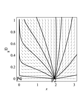
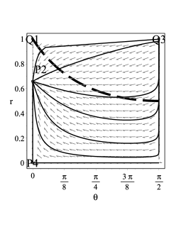
Figure 1: (a) Trajectories in the phase space for the cosmological scenario (4.6)-(4.7), for the parameter choices $\alpha_{1}=-\sqrt{33}$ and $\alpha_{2}=4$, and assuming the matter to be dust ($w_{m}=0$). (b) Projection of the phase space on the “Poincaré plane” $(r,\theta)$. The dashed curve marks the region above which $\Omega_{m}>1$ and the universe may result to future singularities. In this specific example the universe is led to the de Sitter attractor $P_{2}$, while $P_{4}$ is saddle. At infinity, there is not any stable point, and thus the universe cannot result in any form of singularity ($Q_{1}$ and $Q_{2}$ are saddle points ($Q_{2}$ has $\theta<0$ and thus it is not depicted in the plot), while $Q_{3}$ is unstable).

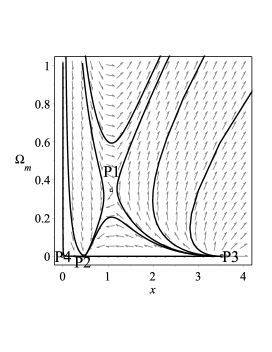
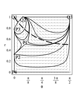
Figure 2: (a) Trajectories in the phase space for the cosmological scenario (4.6)-(4.7), for the parameter choices $\alpha_{1}=\frac{1}{2}$ and $\alpha_{2}=-\frac{1}{2}$, and assuming the matter to be dust ($w_{m}=0$). (b) Projection of the phase space on the “Poincaré plane” $(r,\theta)$. The dashed curve marks the region above which $\Omega_{m}>1$ and the universe may result to future singularities. In this specific example the universe is led to the phantom solution $P_{2}$. At infinity, there is the stable point $Q_{2}$, which corresponds to a future singularity.

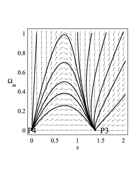
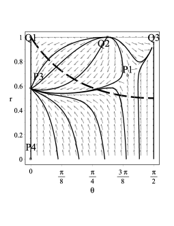
Figure 3: (a) Trajectories in the phase space for the cosmological scenario (4.6)-(4.7), for the parameter choices $\alpha_{1}=3$ and $\alpha_{2}=\frac{3}{2}$, and assuming the matter to be dust ($w_{m}=0$). (b) Projection of the phase space on the “Poincaré plane” $(r,\theta)$. The dashed curve marks the region above which $\Omega_{m}>1$ and the universe may result to future singularities. In this specific example the universe is led to the quintessence solution $P_{3}$. At infinity, there is the stable point $Q_{3}$, which corresponds to a future singularity.

In Fig. 2 we present the phase-space behavior of the autonomous system (4.6)-(4.7) for the choice $\alpha_{1}=\frac{1}{2}$ and $\alpha_{2}=-\frac{1}{2}$ (assuming $w_{m}=0$), and its projection on the “Poincaré plane” $(r,\theta)$. In this case the attractor at the finite region is the phantom solution $P_{2}$. Additionally, the attractor in the infinite region is $Q_{2}$, that is a future singularity.

Finally, in Fig. 3 are present some orbits and the corresponding Poincaré projections for the choice $\alpha_{1}=3$ and $\alpha_{2}=\frac{3}{2}$, with $w_{m}=0$. In this case, the universe is attracted by the quintessence solution $P_{3}$. Furthermore, in the infinite region the attractor is $Q_{3}$, that is a future singularity.

6 Conclusions

In the present work we studied the dynamical behavior of the recently proposed scenario of $f(T,T_{G})$ cosmology [55]. This class of modified gravity is based on the quadratic torsion scalar $T$, which is the Lagrangian of the teleparallel equivalent of General Relativity, as well as on the new quartic torsion scalar $T_{G}$, which is the teleparallel equivalent of the Gauss-Bonnet term. Obviously, $f(T,T_{G})$ theories are more general and cannot be spanned by the simple $f(T)$ ones, and additionally they are different from $f(R,G)$ class of curvature modified gravity too.

Without loss of generality, as a simple, but non-trivial example, capable of revealing the advantages and the new features of the theory, we considered a model where $T$ and $T_{G}$ corrections are of the same order, and thus expected to play an important role at late times. We performed for a spatially flat universe the complete and detailed phase-space behavior, both in the finite and infinite regions, calculating additionally also the values of basic observables such is the various density parameters, the deceleration parameter and the dark energy equation-of-state parameter.

This scenario exhibits interesting cosmological behaviors. In particular, depending on the model parameters, the universe can result in a dark energy dominated accelerating solution and the dark energy equation-of-state parameter can lie in the quintessence regime, it can be equal to the cosmological constant value $-1$, or it can even lie in the phantom regime. Additionally, it can result in a dark energy - dark matter scaling solution, and thus it can alleviate the coincidence problem. Finally, under certain parameter choices the universe can result to Big Rip, sudden, or other form of singularities, as it is usual in many modified gravitational theories. Definitely, before the scenario at hand can be considered as a good candidate for the description of Nature, a detailed confrontation with observations should be performed. In particular, one should use data from local gravity experiments (Solar System observations), as well as type Ia Supernovae (SNIa), Baryon Acoustic Oscillations (BAO), and Cosmic Microwave Background (CMB) radiation data, in order to impose constraints on the model. These necessary investigations lie beyond the scope of the present work and are left for a future project.

Appendix A Stability of the finite critical points

For the critical points $(x_{c},\Omega_{mc})$ of the autonomous system (4.6)-(4.7), presented in Table 1, the coefficients of the perturbation equations form a $2\times 2$ matrix ${\bf{Q}}$, which reads:

$${\bf{Q}}_{11} = \frac{\alpha_{1}(4\alpha_{2}-3)-9\alpha_{1}x^{2}-12x(\Omega_{m}-1)}{2\alpha_{1}\alpha_{2}}$$

$${\bf{Q}}_{12} = -\frac{3x^{2}}{\alpha_{1}\alpha_{2}}$$

$${\bf{Q}}_{21} = -\frac{6x\Omega_{m}}{\alpha_{2}}$$

$${\bf{Q}}_{22} = -\frac{\alpha_{2}+3x^{2}-3}{\alpha_{2}}$$

Thus, we can straightforwardly see that using the explicit critical points shown in Table 1, the matrix ${\bf{Q}}$ acquires a simple form that allows for an easy calculation of its eigenvalues. Hence, by examining the sign of the real parts of these eigenvalues, we can classify the corresponding critical point. In particular, if all eigenvalues of a critical point have positive real parts then this point is unstable, if they all have negative real parts then it is stable, and if they change sign then it is a saddle one. In the following we present the results for each separate point.

Point $P_{1}$ has the coordinates

$$P_{1}:(x,\Omega_{m})=\left(\sqrt{1-\frac{\alpha_{2}}{3}},\frac{\alpha_{1}\sqrt{9-3\alpha_{2}}(6-5\alpha_{2})+6(\alpha_{2}-3)}{6(\alpha_{2}-3)}\right),$$

that is it exists for either $\alpha_{2}=\frac{6}{5}$ or $\frac{6}{5}<\alpha_{2}<3,\,\alpha_{1}\geq-2\sqrt{\frac{3(3-\alpha_{2})}{(5\alpha_{2}-6)^{2}}}$ or $\alpha_{2}<\frac{5}{6},\,\alpha_{1}\leq 2\sqrt{\frac{3(3-\alpha_{2})}{(5\alpha_{2}-6)^{2}}}$. The eigenvalues of the corresponding linearization matrix are

$$\left\{-\frac{\sqrt{\alpha_{1}\left[(336-71\alpha_{2})\alpha_{2}-288\right]+32\sqrt{3}(3-\alpha_{2})^{3/2}}}{4\sqrt{\alpha_{1}}\alpha_{2}}-\frac{3}{4},\right.$$

$$\left.\frac{\sqrt{\alpha_{1}\left[(336-71\alpha_{2})\alpha_{2}-288\right]+32\sqrt{3}(3-\alpha_{2})^{3/2}}}{4\sqrt{\alpha_{1}}\alpha_{2}}-\frac{3}{4}\right\}.$$ (A.1)

Therefore, $P_{1}$ is a stable spiral for

$$\alpha_{2}<3,\ \ -32\sqrt{3}\sqrt{\frac{(3-\alpha_{2})^{3}}{\left(71\alpha_{2}^{2}-336\alpha_{2}+288\right)^{2}}}<\alpha_{1}<0,$$

or

$$\alpha_{1}<0,\alpha_{2}\leq\frac{1}{71}\left(168-36\sqrt{6}\right)\lesssim 1.12421.$$

Otherwise it is a saddle (we have excluded the parameter values that leads to non-hyperbolic critical points).

Point $P_{2}$ has the coordinates

$$P_{2}:(x,\Omega_{m})=\left(\frac{3-\sqrt{3\alpha_{1}^{2}(4\alpha_{2}-3)+9}}{3\alpha_{1}},0\right),$$

that is it exists for either $\alpha_{2}<\frac{3}{4},0<\alpha_{1}\leq\sqrt{\frac{3}{3-4\alpha_{2}}}$ or $\alpha_{1}\neq 0,\alpha_{2}=\frac{3}{4}$ or $\alpha_{2}>\frac{3}{4},\alpha_{1}<0$. The eigenvalues of the linearization matrix are

$$\!\!\!\left\{\frac{2\sqrt{3\alpha_{1}^{2}(4\alpha_{2}-3)+9}}{\alpha_{1}^{2}\alpha_{2}}-\frac{6}{\alpha_{1}^{2}\alpha_{2}}+\frac{6}{\alpha_{2}}-5,\,\frac{\sqrt{3\alpha_{1}^{2}(4\alpha_{2}-3)+9}}{\alpha_{1}^{2}\alpha_{2}}-\frac{3}{\alpha_{1}^{2}\alpha_{2}}+\frac{3}{\alpha_{2}}-4\right\}.$$ (A.2)

Hence, it is an stable node for either

$$\alpha_{2}<0,\ \ 0<\alpha_{1}<2\sqrt{\frac{3(3-\alpha_{2})}{(5\alpha_{2}-6)^{2}}}$$

or

$$\frac{6}{5}<\alpha_{2}\leq 3,\ \ \alpha_{1}<-2\sqrt{\frac{3(3-\alpha_{2})}{(5\alpha_{2}-6)^{2}}}$$

or

$$\alpha_{2}>3,\ \ \alpha_{1}<0.$$

Additionally, it is unstable node for

$$0<\alpha_{2}<\frac{3}{4},\ \ 0<\alpha_{1}<\sqrt{\frac{3}{3-4\alpha_{2}}}.$$

Finally, for the remaining parameter range in the hyperbolic domain, the point behaves as a saddle.

Point $P_{3}$ has the coordinates

$$P_{3}:(x,\Omega_{m})=\left(\frac{3+\sqrt{3\alpha_{1}^{2}(4\alpha_{2}-3)+9}}{3\alpha_{1}},0\right),$$

that is it exists for $\alpha_{2}<\frac{3}{4},\,0<\alpha_{1}\leq\sqrt{\frac{3}{3-4\alpha_{2}}}$ or $\alpha_{2}\geq\frac{3}{4},\alpha_{1}>0$. The eigenvalues of the corresponding linearization matrix are

$$\left\{-\frac{2\sqrt{3}\sqrt{4\alpha_{1}^{2}\alpha_{2}-3\alpha_{1}^{2}+3}}{\alpha_{1}^{2}\alpha_{2}}-\frac{6}{\alpha_{1}^{2}\alpha_{2}}+\frac{6}{\alpha_{2}}-5,\,-\frac{\sqrt{3}\sqrt{4\alpha_{1}^{2}\alpha_{2}-3\alpha_{1}^{2}+3}}{\alpha_{1}^{2}\alpha_{2}}-\frac{3}{\alpha_{1}^{2}\alpha_{2}}+\frac{3}{\alpha_{2}}-4\right\}.$$ (A.3)

That is, it is stable node for

$$\alpha_{1}>0,\ \ \alpha_{2}\geq\frac{6}{5},$$

it is unstable node for

$$\alpha_{2}<0,\ \ 0<\alpha_{1}<\frac{\sqrt{3}}{\sqrt{3-4\alpha_{2}}},$$

otherwise it is a saddle with the exclusion of the parameter values that leads to non-hyperbolic critical point.

Point $P_{4}$ has the coordinates $P_{4}:(x,\Omega_{m})=(0,0)$ and it exists always. The eigenvalues of the linearization matrix read

$$\left\{2-\frac{3}{2\alpha_{2}},\,\frac{3}{\alpha_{2}}-1\right\}.$$

Therefore, it is unstable node for $\frac{3}{4}<\alpha_{2}<3$, it is non-hyperbolic for $\alpha_{2}\in\left\{\frac{3}{4},3\right\}$, otherwise it is a saddle.

The above results are summarized in Table 4.

Cr. P.	$x$	$\Omega_{m}$	Existence	$\nu_{1}$	$\nu_{2}$
$P_{1}$	$\sqrt{1-\frac{\alpha_{2}}{3}}$	$\Omega_{m1}$	$\alpha_{2}=\frac{6}{5}$ or	$-\frac{\sqrt{\alpha_{1}\left[(336-71\alpha_{2})\alpha_{2}-288\right]+32\sqrt{3}(3-\alpha_{2})^{3/2}}}{4\sqrt{\alpha_{1}}\alpha_{2}}-\frac{3}{4}$	$\frac{\sqrt{\alpha_{1}\left[(336-71\alpha_{2})\alpha_{2}-288\right]+32\sqrt{3}(3-\alpha_{2})^{3/2}}}{4\sqrt{\alpha_{1}}\alpha_{2}}-\frac{3}{4}$
			$\frac{6}{5}<\alpha_{2}<3,-2\sqrt{\frac{3(3-\alpha_{2})}{(-6+5\alpha_{2})^{2}}}\leq\alpha_{1}\leq 0$
			or $\alpha_{2}=\frac{6}{5}$
			or $\alpha_{2}<\frac{6}{5},0\leq\alpha_{1}\leq 2\sqrt{\frac{3(3-\alpha_{2})}{(-6+5\alpha_{2})^{2}}}$
$P_{2}$	$\frac{3-\sqrt{3\alpha_{1}^{2}(4\alpha_{2}-3)+9}}{3\alpha_{1}}$	$0$	$\alpha_{2}<\frac{3}{4},0<\alpha_{1}\leq\sqrt{\frac{3}{3-4\alpha_{2}}}$ or	$\frac{2\sqrt{3\alpha_{1}^{2}(4\alpha_{2}-3)+9}}{\alpha_{1}^{2}\alpha_{2}}-\frac{6}{\alpha_{1}^{2}\alpha_{2}}+\frac{6}{\alpha_{2}}-5$	$\frac{\sqrt{3\alpha_{1}^{2}(4\alpha_{2}-3)+9}}{\alpha_{1}^{2}\alpha_{2}}-\frac{3}{\alpha_{1}^{2}\alpha_{2}}+\frac{3}{\alpha_{2}}-4$
			$\alpha_{1}\neq 0,\alpha_{2}=\frac{3}{4}$ or
			$\alpha_{2}>\frac{3}{4},\alpha_{1}<0$
$P_{3}$	$\frac{3+\sqrt{3\alpha_{1}^{2}(4\alpha_{2}-3)+9}}{3\alpha_{1}}$	$0$	$\alpha_{2}<\frac{3}{4},0<\alpha_{1}\leq\sqrt{\frac{3}{3-4\alpha_{2}}}$ or	$-\frac{2\sqrt{3}\sqrt{4\alpha_{1}^{2}\alpha_{2}-3\alpha_{1}^{2}+3}}{\alpha_{1}^{2}\alpha_{2}}-\frac{6}{\alpha_{1}^{2}\alpha_{2}}+\frac{6}{\alpha_{2}}-5$	$-\frac{\sqrt{3}\sqrt{4\alpha_{1}^{2}\alpha_{2}-3\alpha_{1}^{2}+3}}{\alpha_{1}^{2}\alpha_{2}}-\frac{3}{\alpha_{1}^{2}\alpha_{2}}+\frac{3}{\alpha_{2}}-4$
			$\alpha_{2}\geq\frac{3}{4},\alpha_{1}>0$
$P_{4}$	$0$	$0$	Always	$2-\frac{3}{2\alpha_{2}}$	$\frac{3}{\alpha_{2}}-1$

Table 4: The real and physically interesting critical points at the finite region of the autonomous system (4.6)-(4.7), their existence conditions, and the corresponding eigenvalues $\nu_{1},\nu_{2}$ of the matrix ${\bf{Q}}$ of the perturbation equations. We denote $\Omega_{m1}=\frac{\alpha_{1}\sqrt{9-3\alpha_{2}}(6-5\alpha_{2})+6(\alpha_{2}-3)}{6(\alpha_{2}-3)}$.

Appendix B Stability of the critical points at infinity

We introduce the new coordinates $(r,\theta)$ defined by

$$x=\frac{r}{1-r}\cos\theta$$

$$\Omega_{m}=\frac{r}{1-r}\sin\theta,$$ (B.1)

with $\theta\in\left[0,\frac{\pi}{2}\right]$ and $r\in\left[0,1\right)$. The limit $r\rightarrow 1^{-}$ corresponds to $R^{2}\equiv x^{2}+\Omega_{m}^{2}\rightarrow\infty.$ Note that the physical region of the plane $(r,\theta)$, that is corresponding to $0\leq x,\,0\leq\Omega_{m}\leq 1$, is given by

$$\left\{(r,\theta):0\leq r\leq\frac{1}{2},0\leq\theta\leq\frac{\pi}{2}\right\}\cup\left\{(r,\theta):\frac{1}{2}<r<1,0\leq\theta\leq\arcsin\left(\frac{1-r}{r}\right)\right\}.$$ (B.2)

The leading terms of the equations for $r^{\prime}$ and $\theta^{\prime}$ as $r\rightarrow 1^{-}$ are

$$r^{\prime}\rightarrow\frac{3\cos^{2}(\theta)[\alpha_{1}(\cos(2\theta)-3)-2\sin(2\theta)]}{4\alpha_{1}\alpha_{2}(1-r)}$$ (B.3)

$$\theta^{\prime}\rightarrow-\frac{3\sin(\theta)\cos^{2}(\theta)[\alpha_{1}\cos(\theta)-2\sin(\theta)]}{2\alpha_{1}\alpha_{2}(1-r)^{2}}.$$ (B.4)

Hence, the fixed points at infinity (that is for $r\rightarrow 1^{-}$) are obtained by setting $\theta^{\prime}=0$, and solving for $\theta$.

Let us denote a generic fixed point by $\theta=\theta^{*}$. The stability of this point is studied by analyzing first the stability of the angular coordinates from equation (B.4), and then deducing, from the sign of the equation (B.3), the stability on the radial direction . A fixed point $\theta=\theta^{*}$ is said to be stable if both

$$\frac{d\theta^{\prime}}{d\theta}\left|{}_{\theta=\theta^{*}}\right.<0,r^{\prime}\left|{}_{\theta=\theta^{*}}\right.>0.$$ (B.5)

The first condition implies stability of the angular coordinate $\theta$. The second condition implies that the $r$-values increase before reaching the limit value $r=1$ (that is before the boundary “at infinity” is reached) at the fixed point $\theta=\theta^{*}$. Similarly, a fixed point $\theta=\theta^{*}$ is said to be unstable if both

$$\frac{d\theta^{\prime}}{d\theta}\left|{}_{\theta=\theta^{*}}\right.>0,r^{\prime}\left|{}_{\theta=\theta^{*}}\right.<0.$$ (B.6)

Finally, it is a saddle point if either

$$\frac{d\theta^{\prime}}{d\theta}\left|{}_{\theta=\theta^{*}}\right.>0,r^{\prime}\left|{}_{\theta=\theta^{*}}\right.>0,$$ (B.7)

or

$$\frac{d\theta^{\prime}}{d\theta}\left|{}_{\theta=\theta^{*}}\right.<0,r^{\prime}\left|{}_{\theta=\theta^{*}}\right.<0.$$ (B.8)

In summary, the fixed points of the autonomous system at hand at infinity are the following:

• $Q_{1}:\theta^{*}=0,r^{*}=1,x=\infty,\Omega_{m}=0$.

  Since from the definition (4.4) we have $x=\sqrt{1+\frac{2\alpha_{2}}{3}\left(1+\frac{\dot{H}}{H^{2}}\right)}$, we deduce that the corresponding cosmological solution satisfies $\text{sign}(\alpha_{2}\dot{H})\frac{|\dot{H}|}{H^{2}}\rightarrow\infty,$ or $H\rightarrow 0$ ($\dot{H}$ is bounded, with $\text{sign}(\alpha_{2}\dot{H})>0$). Since $q=w_{DE}=-\text{sgn}(\alpha_{2})\infty$, the point represents a super-accelerated phantom solution for $\alpha_{2}>0$, where eventually the universe ends in Big Rip, sudden or other forms of singularities (depending on whether the singularity is reached at finite or infinite time, what are its features etc.) [68, 69, 70, 71, 72, 73]. For $\alpha_{2}<0$ it is a decelerating solution where the universe asymptotically stops expanding. Since $\left(\frac{d\theta^{\prime}}{d\theta},r^{\prime}\right)|_{\theta=0}=\left(-\frac{3}{2\alpha_{2}},-\frac{3}{2\alpha_{2}}\right)$, we conclude that $Q_{1}$ is always a saddle point.

• $Q_{2}:\theta^{*}=\arctan\left(\frac{\alpha_{1}}{2}\right),\alpha_{1}\neq 0,r^{*}=1,\frac{\Omega_{m}}{x}\rightarrow\frac{\alpha_{1}}{2},x\rightarrow\infty,\Omega_{m}\rightarrow\infty$. Since $0\leq\theta\leq\frac{\pi}{2},$ then $\alpha_{1}>0$. Since $\left(\frac{d\theta^{\prime}}{d\theta},r^{\prime}\right)|_{\theta=\frac{\pi}{2}}=\left(\frac{6}{(1+\alpha_{1}^{2})\alpha_{2}},-\frac{12}{(1+\alpha_{1}^{2})\alpha_{2}}\right)$, we deduce that $Q_{2}$ is unstable for $\alpha_{2}>0$ or stable for $\alpha_{2}<0$, as confirmed in Figure 2. Since at this point $\Omega_{m}$ diverges, it corresponds to some form of future (respectively past) singularity for $\alpha_{2}<0$ (respectively $\alpha_{2}>0$) [68, 69, 70, 71, 72, 73]. Its detailed classification for the various parameter regions lies beyond the scope of the present work.

• $Q_{3}:\theta^{*}=\frac{\pi}{2},r^{*}=1,x=0,\Omega_{m}=\infty$. Since $\left(\frac{d\theta^{\prime}}{d\theta},r^{\prime}\right)|_{\theta=\frac{\pi}{2}}=\left(0,0\right)$, we cannot rely on the linearization to examine the stability, and therefore, we need to resort to numerical examination (see Figures 1, 2). Since at this point $\Omega_{m}$ diverges, it corresponds to some form of future, past or intermediate singularity [68, 69, 70, 71, 72, 73].

The above results are summarized in Table 5.

Cr. P.	$\theta^{*}$	$\frac{d\theta^{\prime}}{d\theta}\left|{}_{\theta=\theta^{*}}\right.$	$r^{\prime}\left|{}_{\theta=\theta^{*}}\right.$	Stability
$Q_{1}$	$0$	$-\frac{3}{2\alpha_{2}}$	$-\frac{3}{2\alpha_{2}}$	saddle point
$Q_{2}$	$\arctan\left(\frac{\alpha_{1}}{2}\right)$	$\frac{6}{(1+\alpha_{1}^{2})\alpha_{2}}$	$-\frac{12}{(1+\alpha_{1}^{2})\alpha_{2}}$	unstable for $\alpha_{2}>0$
				stable for $\alpha_{2}<0$
$Q_{3}$	$\frac{\pi}{2}$	$0$	$0$	see numerical elaboration

Table 5: The real critical points of the autonomous system (4.6)-(4.7) at infinity, their existence conditions, the corresponding values of $\frac{d\theta^{\prime}}{d\theta}$ and $r^{\prime}$, and the resulting stability conditions.

References

• [1] E. J. Copeland, M. Sami and S. Tsujikawa, Dynamics of dark energy, Int. J. Mod. Phys.  D 15, 1753 (2006), [arXiv:hep-th/0603057].
• [2] Y. -F. Cai, E. N. Saridakis, M. R. Setare and J. -Q. Xia, Quintom Cosmology: Theoretical implications and observations, Phys. Rept.  493, 1 (2010), [arXiv:0909.2776].
• [3] S. Capozziello and M. De Laurentis, Extended Theories of Gravity, Phys. Rept.  509, 167 (2011), [arXiv:1108.6266].
• [4] V. Sahni and A. Starobinsky, Reconstructing Dark Energy, Int. J. Mod. Phys. D 15, 2105 (2006), [arXiv:astro-ph/0610026].
• [5] S. ’i. Nojiri and S. D. Odintsov, Modified gravity with negative and positive powers of the curvature: Unification of the inflation and of the cosmic acceleration, Phys. Rev. D 68, 123512 (2003), [arXiv:hep-th/0307288].
• [6] A. Unzicker and T. Case, Translation of Einstein’s attempt of a unified field theory with teleparallelism, [arXiv:physics/0503046].
• [7] K. Hayashi and T. Shirafuji, New general relativity, Phys. Rev.  D 19, 3524 (1979) [Addendum-ibid.  D 24, 3312 (1982)].
• [8] R. Aldrovandi and J. G. Pereira, Teleparallel Gravity: An Introduction, Springer, Dordrecht (2013).
• [9] J. W. Maluf, The teleparallel equivalent of general relativity, Annalen Phys.  525, 339 (2013), [arXiv:1303.3897].
• [10] A. De Felice and S. Tsujikawa, f(R) theories, Living Rev. Rel.  13, 3 (2010), [arXiv:1002.4928].
• [11] S. ’i. Nojiri and S. D. Odintsov, Unified cosmic history in modified gravity: from F(R) theory to Lorentz non-invariant models, Phys. Rept.  505, 59 (2011), [arXiv:1011.0544].
• [12] R. Ferraro and F. Fiorini, Modified teleparallel gravity: Inflation without inflaton, Phys. Rev. D 75, 084031 (2007), [arXiv:gr-qc/0610067].
• [13] G. R. Bengochea and R. Ferraro, Dark torsion as the cosmic speed-up, Phys. Rev. D 79, 124019 (2009), [arXiv:0812.1205].
• [14] E. V. Linder, Einstein’s Other Gravity and the Acceleration of the Universe, Phys. Rev.  D 81, 127301 (2010), [arXiv:1005.3039].
• [15] S. H. Chen, J. B. Dent, S. Dutta and E. N. Saridakis, Cosmological perturbations in f(T) gravity, Phys. Rev. D 83, 023508 (2011), [arXiv:1008.1250].
• [16] J. B. Dent, S. Dutta, E. N. Saridakis, f(T) gravity mimicking dynamical dark energy. Background and perturbation analysis, JCAP 1101, 009 (2011) [arXiv:1010.2215].
• [17] R. Zheng and Q. G. Huang, Growth factor in f(T) gravity, JCAP 1103, 002 (2011), [arXiv:1010.3512].
• [18] Y. -F. Cai, S. -H. Chen, J. B. Dent, S. Dutta, E. N. Saridakis, Matter Bounce Cosmology with the f(T) Gravity, Class. Quant. Grav.  28, 2150011 (2011), [arXiv:1104.4349].
• [19] M. Sharif, S. Rani, F(T) Models within Bianchi Type I Universe, Mod. Phys. Lett.  A26, 1657 (2011), [arXiv:1105.6228].
• [20] M. Li, R. X. Miao and Y. G. Miao, Degrees of freedom of $f(T)$ gravity, JHEP 1107, 108 (2011), [arXiv:1105.5934].
• [21] C. G. Boehmer, A. Mussa and N. Tamanini, Existence of relativistic stars in f(T) gravity, Class. Quant. Grav.  28, 245020 (2011), [arXiv:1107.4455].
• [22] S. Capozziello, V. F. Cardone, H. Farajollahi and A. Ravanpak, Cosmography in f(T)-gravity, Phys. Rev.  D 84, 043527 (2011), [arXiv:1108.2789].
• [23] M. H. Daouda, M. E. Rodrigues and M. J. S. Houndjo, Static Anisotropic Solutions in f(T) Theory, [arXiv:1109.0528].
• [24] C. -Q. Geng, C. -C. Lee, E. N. Saridakis and Y. -P. Wu, ’Teleparallel’ Dark Energy, Phys. Lett. B 704, 384 (2011), [arXiv:1109.1092].
• [25] Y. P. Wu and C. Q. Geng, Primordial Fluctuations within Teleparallelism, Phys. Rev. D 86, 104058 (2012), [arXiv:1110.3099].
• [26] P. A. Gonzalez, E. N. Saridakis and Y. Vasquez, Circularly symmetric solutions in three-dimensional Teleparallel, f(T) and Maxwell-f(T) gravity, [arXiv:1110.4024].
• [27] H. Wei, X. J. Guo and L. F. Wang, Noether Symmetry in $f(T)$ Theory, Phys. Lett.  B 707, 298 (2012), [arXiv:1112.2270].
• [28] K. Atazadeh and F. Darabi, $f(T)$ cosmology via Noether symmetry, [arXiv:1112.2824].
• [29] H. Farajollahi, A. Ravanpak and P. Wu, Cosmic acceleration and phantom crossing in $f(T)$-gravity, Astrophys. Space Sci.  338, 23 (2012), [arXiv:1112.4700].
• [30] K. Karami and A. Abdolmaleki, Generalized second law of thermodynamics in f(T)-gravity, [arXiv:1201.2511].
• [31] L. Iorio and E. N. Saridakis, Solar system constraints on f(T) gravity, [arXiv:1203.5781].
• [32] V. F. Cardone, N. Radicella and S. Camera, Accelerating f(T) gravity models constrained by recent cosmological data, Phys. Rev. D 85, 124007 (2012), [arXiv:1204.5294].
• [33] S. Capozziello, P. A. Gonzalez, E. N. Saridakis and Y. Vasquez, Exact charged black-hole solutions in D-dimensional f(T) gravity: torsion vs curvature analysis, JHEP 1302 (2013) 039, [arXiv:1210.1098].
• [34] M. Jamil, D. Momeni and R. Myrzakulov, Wormholes in a viable f(T) gravity, Eur. Phys. J. C 72, 2267 (2012), [arXiv:1212.6017].
• [35] Y. C. Ong, K. Izumi, J. M. Nester and P. Chen, Problems with Propagation and Time Evolution in f(T) Gravity, Phys. Rev. D 88 (2013) 2, 024019, [arXiv:1303.0993].
• [36] J. Amoros, J. de Haro and S. D. Odintsov, Bouncing Loop Quantum Cosmology from $F(T)$ gravity, Phys. Rev. D 87, 104037 (2013), [arXiv:1305.2344].
• [37] G. Otalora, Cosmological dynamics of tachyonic teleparallel dark energy, Phys. Rev. D 88, 063505 (2013), [arXiv:1305.5896].
• [38] C. -Q. Geng, J. -A. Gu and C. -C. Lee, Singularity Problem in Teleparallel Dark Energy Models, Phys. Rev. D 88, 024030 (2013), [arXiv:1306.0333].
• [39] S. Nesseris, S. Basilakos, E. N. Saridakis and L. Perivolaropoulos, Viable f(T) models are practically indistinguishable from LCDM, Phys. Rev. D 88, 103010 (2013), [arXiv:1308.6142].
• [40] K. Bamba, S. Capozziello, M. De Laurentis, S. ’i. Nojiri and D. Sáez-Gómez, No further gravitational wave modes in $F(T)$ gravity, Phys. Lett. B 727, 194 (2013), [arXiv:1309.2698].
• [41] G. G. L. Nashed, $f(T)$ gravity theories and local Lorentz transformation, [arXiv:1403.6937].
• [42] T. Harko, F. S. N. Lobo, G. Otalora and E. N. Saridakis, Nonminimal torsion-matter coupling extension of f(T) gravity, Phys. Rev. D 89, 124036 (2014), [arXiv:1404.6212].
• [43] T. Harko, F. S. N. Lobo, G. Otalora and E. N. Saridakis, $f(T,\mathcal{T})$ gravity and cosmology, [arXiv:1405.0519].
• [44] J. T. Wheeler, Symmetric Solutions to the Gauss-Bonnet Extended Einstein Equations, Nucl. Phys. B 268, 737 (1986).
• [45] I. Antoniadis, J. Rizos and K. Tamvakis, Singularity - free cosmological solutions of the superstring effective action, Nucl. Phys. B 415, 497 (1994), [arXiv:hep-th/9305025].
• [46] S. ’i. Nojiri, S. D. Odintsov and M. Sasaki, Gauss-Bonnet dark energy, Phys. Rev. D 71, 123509 (2005), [arXiv:hep-th/0504052].
• [47] S. ’i. Nojiri and S. D. Odintsov, Modified Gauss-Bonnet theory as gravitational alternative for dark energy, Phys. Lett. B 631, 1 (2005), [arXiv:hep-th/0508049].
• [48] A. De Felice and S. Tsujikawa, Construction of cosmologically viable f(G) dark energy models, Phys. Lett. B 675, 1 (2009), [arXiv:0810.5712].
• [49] D. Lovelock, The Einstein tensor and its generalizations, J. Math. Phys.  12, 498 (1971).
• [50] N. Deruelle and L. Farina-Busto, The Lovelock Gravitational Field Equations in Cosmology, Phys. Rev. D 41, 3696 (1990).
• [51] C. Charmousis, Higher order gravity theories and their black hole solutions, Lect. Notes Phys.  769 (2009) 299, [arXiv:0805.0568].
• [52] P. D. Mannheim and D. Kazanas, Exact Vacuum Solution to Conformal Weyl Gravity and Galactic Rotation Curves, Astrophys. J.  342, 635 (1989).
• [53] E. E. Flanagan, Fourth order Weyl gravity, Phys. Rev. D 74, 023002 (2006), [arXiv:astro-ph/0605504].
• [54] D. Grumiller, M. Irakleidou, I. Lovrekovic and R. McNees, Conformal gravity holography in four dimensions, Phys. Rev. Lett.  112, 111102 (2014), [arXiv:1310.0819].
• [55] G. Kofinas and E. N. Saridakis, Teleparallel equivalent of Gauss-Bonnet gravity and its modifications, [arXiv:1404.2249].
• [56] S. C. Davis, Solar system constraints on f(G) dark energy, [arXiv:0709.4453].
• [57] A. De Felice and S. Tsujikawa, Solar system constraints on f(G) gravity models, Phys. Rev. D 80, 063516 (2009), [arXiv:0907.1830].
• [58] A. Jawad, S. Chattopadhyay and A. Pasqua, Reconstruction of f(G) gravity with the new agegraphic dark-energy model, Eur. Phys. J. Plus 128, 88 (2013).
• [59] L. Perko, Differential Equations and Dynamical Systems, Third Edition, Springer (2001).
• [60] Dynamical Systems in Cosmology, edited by J. Wainwright and G. F. R. Ellis, Cambridge University Press (1997).
• [61] E. J. Copeland, A. R. Liddle and D. Wands, Exponential potentials and cosmological scaling solutions, Phys. Rev.  D 57, 4686 (1998), [arXiv:gr-qc/9711068].
• [62] P. G. Ferreira and M. Joyce, Structure formation with a self-tuning scalar field, Phys. Rev. Lett.  79, 4740 (1997), [arXiv:astro-ph/9707286].
• [63] X. m. Chen, Y. g. Gong and E. N. Saridakis, Phase-space analysis of interacting phantom cosmology, JCAP 0904, 001 (2009), [arXiv:0812.1117].
• [64] S. Cotsakis and G. Kittou, Flat limits of curved interacting cosmic fluids, Phys. Rev. D 88, 083514 (2013), [arXiv:1307.0377].
• [65] R. Giambo and J. Miritzis, Energy exchange for homogeneous and isotropic universes with a scalar field coupled to matter, Class. Quant. Grav.  27 (2010) 095003, [arXiv:0908.3452].
• [66] S. Lynch, Dynamical Systems with Applications using Mathematica, Birkhauser, Boston (2007).
• [67] C. Xu, E. N. Saridakis and G. Leon, Phase-Space analysis of Teleparallel Dark Energy, JCAP 1207, 005 (2012), [arXiv:1202.3781].
• [68] M. Sami and A. Toporensky, Phantom field and the fate of universe, Mod. Phys. Lett. A 19, 1509 (2004), [arXiv:gr-qc/0312009]
• [69] S. ’i. Nojiri, S. D. Odintsov and S. Tsujikawa, Properties of singularities in (phantom) dark energy universe, Phys. Rev. D 71, 063004 (2005), [arXiv:hep-th/0501025]
• [70] F. Briscese, E. Elizalde, S. Nojiri and S. D. Odintsov, Phantom scalar dark energy as modified gravity: Understanding the origin of the Big Rip singularity, Phys. Lett. B 646, 105 (2007), [arXiv:hep-th/0612220].
• [71] K. Bamba, S. ’i. Nojiri and S. D. Odintsov, The Universe future in modified gravity theories: Approaching the finite-time future singularity, JCAP 0810, 045 (2008), [arXiv:0807.2575].
• [72] S. Capozziello, M. De Laurentis, S. Nojiri and S. D. Odintsov, Classifying and avoiding singularities in the alternative gravity dark energy models, Phys. Rev. D 79, 124007 (2009), [arXiv:0903.2753].
• [73] E. N. Saridakis and J. M. Weller, A Quintom scenario with mixed kinetic terms, Phys. Rev. D 81, 123523 (2010), [arXiv:0912.5304].
• [74] G. Kofinas, G. Panotopoulos and T. N. Tomaras, Brane-bulk energy exchange: A Model with the present universe as a global attractor, JHEP 0601, 107 (2006), [arXiv:0510207].