Numerical test of hydrodynamic fluctuation theory in the Fermi-Pasta-Ulam chain

Abstract

Recent work has developed a nonlinear hydrodynamic fluctuation theory for a chain of coupled anharmonic oscillators governing the conserved fields, namely stretch, momentum, and energy. The linear theory yields two propagating sound modes and one diffusing heat mode. In contrast, the nonlinear theory predicts that, at long times, the sound mode correlations satisfy Kardar-Parisi-Zhang (KPZ) scaling, while the heat mode correlations satisfies Lévy-walk scaling. In the present contribution we report on molecular dynamics simulations of Fermi-Pasta-Ulam chains to compute various spatiotemporal correlation functions and compare them with the predictions of the theory. We find very good agreement in many cases, but also some deviations.

I Introduction

It is now general consensus that heat conduction in one-dimensional (1D) momentum conserving systems is anomalous LLP03 ; dhar08 . There are various approaches which lead to this conclusion. The first approach is through direct nonequilibrium molecular dynamics simulations LLP97 ; dhar02 ; grass02 ; casati03 ; mai07 . Consider a system of $N$ particles connected at the ends to heat baths with a small temperature difference $\Delta T$, so that a steady state heat current $J$ flows across the system. Defining the thermal conductivity as $\kappa=JN/\Delta T$ one typically finds

$$\kappa\sim N^{\alpha}$$ (1)

with $0<\alpha<1$, which means that Fourier’s law is not valid. A second approach is to use the Green-Kubo formula relating thermal conductivity to the integral over the equilibrium heat current auto-correlation function. Simulations and several theoretical approaches delfini06 ; narayan ; wang04 ; pereverez03 ; lukkarinen ; BBO ; beijeren find that the correlation function has a slow power law decay $\sim 1/t^{1-\alpha}$ and this again results in a divergent conductivity. Finally, a number of contributions onuttom03 ; zhao06 ; chen11 ; cipriani ; denisov11 ; lepri11 ; dhar13 ; liu14 have studied the decay of equilibrium energy fluctuations or of heat pulses and find that they are super-diffusive. This is understood through phenomenological models in which the energy carriers perform Lévy walks cipriani ; denisov11 ; lepri11 ; dhar13 .

A significant step towards understanding anomalous heat transport in one-dimension was achieved recently in beijeren and extended to anharmonic chains in mendl13 ; spohn13 , where a detailed theory of hydrodynamic fluctuations is developed including several analytic results. The main strength of this theory lies in very detailed predictions which can be verified through direct simulations of microscopic models. Unlike earlier studies which have mainly focused on the thermal conductivity exponent $\alpha$, nonlinear fluctuating hydrodynamics predicts the scaling forms of various correlation functions, including prescriptions to compute the non-universal parameters for a given microscopic model. The hydrodynamic theory is based on several assumptions and hence there is a need to check the theory through a comparison with results from molecular dynamic simulations. This is the aim of our contribution. In a recent paper mendl14 results are discussed for hard point particle systems either interacting via the so-called shoulder potential or with alternating masses. Here we consider Fermi-Pasta-Ulam (FPU) chains, report on simulation results for equilibrium time correlations in different parameter regimes, and compare with the theory.

There is a large body of work which addresses the equilibration in FPU chains berman ; benettin ; ruffo . As in our study they start from random initial data. However they consider non-equilibrium initial conditions at very low energy. In contrast we investigate the decay of time correlations with initial data chosen from a thermal distribution at a moderate temperature. The correlation functions are obtained by performing an average over these initial conditions.

Let us first summarize the results of the theory in spohn13 . Consider $N$ particles with positions and momenta described by the variables $\{q(x),p(x)\}$, for $x=1,\ldots,N$, and moving on a periodic ring of size $L$ such that $q({N+1})=q(1)+L$ and $p({N+1})=p(1)$. Defining the “stretch” variables $r(x)=q(x+1)-q(x)$, the anharmonic chain is described by the following Hamiltonian with nearest neighbor interactions

$$H=\sum_{x=1}^{N}\epsilon(x),\quad\epsilon(x)=\frac{p^{2}(x)}{2}+V[r(x)]~{},$$ (2)

where the particles are assumed to have unit mass. From the Hamiltonian equations of motion one conludes that stretch $r(x)$, momentum $p(x)$, and energy $\epsilon(x)$ are locally conserved and satisfy the following equations of motion

$$\frac{\partial r(x,t)}{\partial t} =\frac{\partial p(x,t)}{\partial x},$$

$$\frac{\partial p(x,t)}{\partial t} =-\frac{\partial{P}(x,t)}{\partial x},$$

$$\frac{\partial e(x,t)}{\partial t} =-\frac{\partial}{\partial x}[p(x,t){P}(x,t)]~{},$$ (3)

where ${P}(x)=-dV(r)/dr|_{x-1}$ is the local force and $\partial f/\partial x=f(x+1)-f(x)$ denotes the discrete derivative. Assume that the system is in a state of thermal equilibrium at zero total average momentum in such a way that, respectively, the average energy and average stretch are fixed by the temperature ($T=\beta^{-1}$) and pressure ($P$) of the chain. This corresponds to an ensemble defined by the distribution

$$\mathcal{P}(\{p(x),r(x)\})=\prod_{x=1}^{N}\frac{e^{-\beta[p_{x}^{2}/2+V(r_{x})+Pr_{x}]}}{Z_{x}}~{},\quad Z_{x}=\int_{-\infty}^{\infty}dp\int_{-\infty}^{\infty}dre^{-\beta[p^{2}/2+V(r)+Pr]}~{}.$$ (4)

Now consider small fluctuations of the conserved quantities about their equilibrium values, $u_{1}(x,t)=r(x,t)-\langle r\rangle_{eq}$, $u_{2}(x,t)=p(x,t)$ and $u_{3}(x,t)=\epsilon(x,t)-\langle\epsilon\rangle_{eq}$. The fluctuating hydrodynamic equations for the field $\vec{u}=(u_{1},u_{2},u_{3})$ are now written by expanding the conserved currents in Eq. (3) to second order in the nonlinearity and then adding dissipation and noise terms to ensure thermal equilibration. Thereby one arrives at the noisy hydrodynamic equations

$$\partial_{t}u_{\alpha}=-\partial_{x}\left[A_{\alpha\beta}u_{\beta}+H^{\alpha}_{\beta\gamma}u_{\beta}u_{\gamma}-\partial_{x}\widetilde{D}_{\alpha\beta}u_{\beta}+\widetilde{B}_{\alpha\beta}\xi_{\beta}\right]~{}.~{}~{}~{}~{}$$ (5)

The noise and dissipation matrices, $\widetilde{B},\widetilde{D}$, are related by the fluctuation-dissipation relation $\widetilde{D}C+C\widetilde{D}=\widetilde{B}\widetilde{B}^{T}$, where the matrix $C$ corresponds to equilibrium correlations and has elements $C_{\alpha\beta}(x)=\langle u_{\alpha}(x,0)u_{\beta}(0,0)\rangle$.

We switch to normal modes of the linearized equations through the transformation $(\phi_{-1},\phi_{0},\phi_{1})=\vec{\phi}=R\vec{u}$, where the matrix $R$ acts only on the component index and diagonalizes $A$, i.e.  $RAR^{-1}={\rm diag}(-c,0,c)$. The diagonal form implies that there are two sound modes, $\phi_{\pm}$, traveling at speed $c$ in opposite directions and one stationary but decaying heat mode, $\phi_{0}$. The quantities of interest are the equilibrium spatiotemporal correlation functions $C_{ss^{\prime}}(x,t)=\langle\phi_{s}(x,t)\phi_{s^{\prime}}(0,0)\rangle$, where $s,s^{\prime}=-,0,+$. Because the modes separate linearly in time, one argues that they decouple into three single component equations. These have the structure of the noisy Burgers equation, for which the exact scaling function, denoted by $f_{\mathrm{KPZ}}$, is available. This works well for the sound peaks. But for the heat peak the self-coupling coefficient vanishes whatever the interaction potential. Thus one has to study the sub-leading corrections, which at present can be done only within mode-coupling approximation, resulting in the symmetric Lévy-walk distribution. While this is an approximation, it seems to be very accurate. For the generic case of non-zero pressure, i.e. $P\neq 0$, which corresponds either to asymmetric inter-particle potentials or to an externally applied stress, the prediction for the left moving, resp. right moving, sound peaks and the heat mode are

$$C_{\mp\mp}(x,t) =\frac{1}{(\lambda_{s}t)^{2/3}}~{}f_{\mathrm{KPZ}}\left[~{}\frac{(x\pm ct)}{(\lambda_{s}t)^{2/3}}~{}\right]~{},$$ (6)

$$C_{00}(x,t) =\frac{1}{(\lambda_{e}t)^{3/5}}~{}f^{5/3}_{\mathrm{LW}}\left[~{}\frac{x}{(\lambda_{e}t)^{3/5}}~{}\right]~{}.$$ (7)

$f_{\mathrm{KPZ}}(x)$ is the KPZ scaling function discussed in spohn13 ; prahoferspohn2004 , and tabulated in prahofertable . $f_{\mathrm{LW}}^{\nu}(x)$ is the Fourier transform of the Lévy characteristic function $e^{-|k|^{\nu}}$. For an even potential at $P=0$, all self-coupling coefficients vanish and, within mode-coupling approximation, one obtains

$$C_{\mp\mp}(x,t) =\frac{1}{{(\lambda^{0}_{s}t)}^{1/2}}f_{\mathrm{G}}\left[~{}\frac{(x\pm ct)}{(\lambda_{s}^{0}t)^{1/2}}~{}\right]~{},$$ (8)

$$C_{00}(x,t) =\frac{1}{(\lambda_{e}^{0}t)^{2/3}}~{}f^{3/2}_{\mathrm{LW}}\left[~{}\frac{x}{(\lambda_{e}^{0}t)^{2/3}}~{}\right]~{},$$ (9)

where $f_{\mathrm{G}}(x)$ is the unit Gaussian with zero mean. In a recent contribution JKO , a model with the same signatures is studied and their exact result agrees with the mode-coupling predictions (8), (9).

For the non-zero pressure case, the scaling coefficients $\lambda_{s}$ and $\lambda_{e}$ for the sound and heat mode respectively are given by

$$\lambda_{s} =2\sqrt{2}|G^{1}_{11}|~{},$$

$$\lambda_{e} ={\lambda_{s}}^{-2/3}C^{-1/3}{(G^{0}_{11})}^{2}a_{e}~{},$$ (10)

where $a_{e}=2\sqrt{3}~{}\Gamma(1/3)\int^{\infty}_{-\infty}~{}dx{f_{KPZ}(x)}^{2}=3.167...$ is a model-independent numerical constant, and the matrices $G^{\alpha}$ are related to the nonlinear coupling matrices $H^{\alpha}$ through the normal mode transformation defined by $R$ (see Appendix for details).
For the case of an even potential at zero pressure, the sound peaks are diffusive. The coefficient $\lambda_{s}^{0}$ is a transport coefficient which in principle is determined through a Green-Kubo formula. Thus an explicit formula is unlikely and $\lambda_{s}^{0}$ remains undetermined by the theory. In contrast, for the generic case the leading coefficients are obtained from static averages. The heat mode couples to the sound modes and its exact scaling coefficient is

$$\lambda_{e}^{0}=(\lambda_{s}^{0})^{-1/2}c^{-1/2}{(G^{0}_{11})}^{2}{(4\pi)}^{2}a_{e}^{0},~{}$$ (11)

where $a_{e}^{0}=4\int^{\infty}_{0}dt~{}t^{-1/2}cos(t)\int^{\infty}_{-\infty}dx~{}{f_{G}(x)}^{2}=\sqrt{2}$. From a simulation of the microscopic dynamics one obtains $\lambda_{s}^{0}$, and from there one calculates $\lambda_{e}^{0}$ using the above formula. In the following section, we discuss the results of our molecular dynamics simulations in computing the correlation functions and compare them with the scaling predictions.

II Molecular Dynamics Simulations

To verify the predictions from hydrodynamics, we consider the FPU $\alpha$-$\beta$ model described by the following inter-particle potential

$$V(r)=k_{2}\frac{r^{2}}{2}+k_{3}\frac{r^{3}}{3}+k_{4}\frac{r^{4}}{4}~{}.$$ (12)

The set of variables $\{r(x),p(x)\}$, $x=1,2,\ldots,N$, are evolved according to the equations of motion

$$\dot{r}(x)=p(x+1)-p(x),~{}~{}\dot{p}(x)=V^{\prime}(r(x))-V^{\prime}(r(x-1))~{},$$ (13)

with initial conditions chosen from the distribution given by Eq. (4). For the product measure it is easy to generate the initial distribution directly and one does not need to dynamically equilibrate the system. The integrations have been done using both the velocity-Verlet algorithm AT87 and also through the fourth order Runge-Kutta algorithm and we do not find any significant difference. The full set of two-point correlation functions were obtained by averaging over around $10^{6}-10^{7}$ initial conditions. Here we present results for four different parameter sets.

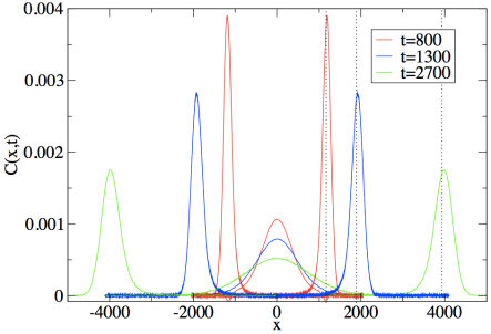
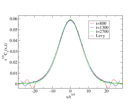
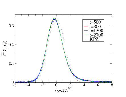
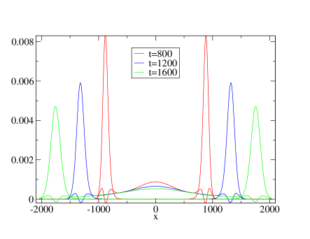
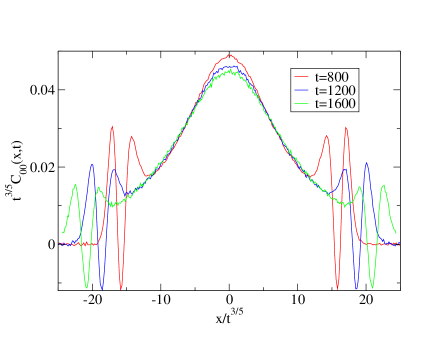
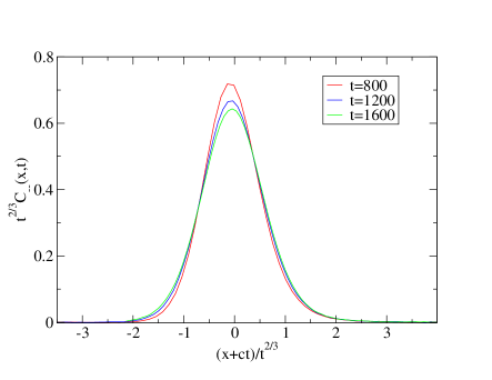
Set I: $k_{2}=1.0,k_{3}=2.0,k_{4}=1.0,T=0.5,P=1.0$. These are the set of parameters used in mendl13 for the numerical solutions of the mode-coupling equations. In Fig. (1) we show the heat mode correlation $C_{00}$ and the sound mode correlations $C_{--},C_{++}$ at three different times. The speed of sound is $c=1.45468...$ The dotted vertical lines in the figure indicate the distances $\ell=ct$. The sound peaks are at their anticipated positions. In Fig. (2) we show the heat mode and the left moving sound mode after scaling according to the predictions in Eqs. (6,7). One can see that the scaling is very good. For comparison we have also plotted a Lévy-stable distribution and the KPZ scaling function prahofertable , and find that the agreement is good for the heat mode but not so good for the sound mode. One observes a still significant asymmetry in the sound mode correlations, contrary to what one would expect from the symmetric KPZ function.

From our numerical fits shown in Fig. (2) we obtain the estimates $\lambda_{s}=2.05$ and $\lambda_{e}=13.8$. The theoretical values based on Eq. (10) are $\lambda_{s}=0.675$ and $\lambda_{e}=1.97$ (see Appendix), which thus deviates significantly from the numerical estimates obtained from the simulations. The disagreement could mean that, for this choice of parameters, we are still not in the asymptotic hydrodynamic regime. We expect that the scaling will improve if the heat and sound mode are more strongly decoupled. To check this, we simulated a set of parameters where the sound speed is higher and the separation between the sound and heat modes is more pronounced. We now discuss this case.

Figure 1: Set I: The parameters of the simulation are $k_{2}=1,~{}k_{3}=2,~{}k_{4}=1,~{}T=0.5$, $P=1$ and system size $N=8192$. Correlation functions for the heat mode and the two sound modes at three different times. At the latest time we see that the heat and sound modes are well separated. The speed of sound is $c=1.45468$.

Figure 2: Set I: Same parameters as in Fig.(1). Scaled plots of heat mode and left moving sound mode correlations, at different times, using a Lévy-type-scaling for the heat mode and KPZ-type scaling for the sound mode. We see here that the collapse of different time data is very good. The fit to the Lévy-stable distribution with $\lambda_{e}=13.8$ is quite good, while the fit to the KPZ scaling function with $\lambda_{s}=2.05$ is not convincing.

Figure 3: Set I: Same parameters as in Fig.(1). Scaled plots of heat mode and right moving sound mode correlations, at different times, using a diffusive scaling ansatz. We see here that the collapse of different time data is not very good and so clearly the modes are not diffusive.

Figure 4: Set II: Heat and sound mode correlations at three different times for the parameter set as in Fig. (1) but with $T=5.0$ and system size $16384$. The speed of sound in this case was $c=1.80293$. In this case we see that the separation of the heat and sound modes is faster and more pronounced than for the parameter set of Fig. (1).

Figure 5: Set II: Same parameters as in Fig.(4). Scaled plots of heat mode and left moving sound mode correlations at different times, using a Lévy-type-scaling for the heat mode and KPZ-type scaling for the sound mode. We see here that the collapse of different time data is very good. Again we find a very good fit to the Lévy-stable distribution with $\lambda_{e}=5.86$ while the fit to the KPZ scaling function, with $\lambda_{s}=0.46$, is not yet perfect.

Figure 6: Set III: Low temperature case - The parameters of the Hamiltonian are $k_{2}=1,~{}k_{3}=-1,~{}k_{4}=1,~{}T=0.1$, $P=0.07776$ and $N=4096$. In this plot we show the heat mode correlation and the two sound mode correlations at three different times. In this case the separation between heat and sound modes is less pronounced.

Figure 7: Set III: Same set of parameters as in Fig. (6). Scaled plots of heat mode and left moving sound mode correlations, at different times, using a Lévy-type-scaling for the heat mode and KPZ-type scaling for the sound mode. We see here that the collapse of different time data for the heat mode is reasonably good.

Figure 8: Set IV: Even potential, zero pressure case - The parameters of the Hamiltonian are $k_{2}=1,k_{3}=0,k_{4}=1$, $P=0$, $T=1$ and $N=8192$. The scaling used here corresponds to Eqs. (8,9), with $\lambda_{s}^{0}=0.416$ and $\lambda_{e}^{0}=3.18$.

Figure 9: Set IV: Parameters same as in Fig. (8). The scaling used here corresponds to Eqs. (6,7). We see that the collapse is not as good as in Fig. (8).

Figure 10: Set V: Even potential, finite pressure case - The parameters of the Hamiltonian are $k_{2}=1,k_{3}=0,k_{4}=1$, $P=1$, $T=1$ and $N=3200$. In this case the scaling corresponding to Eqs. (6,7) is used in this figure and we have checked that the scaling in Eqs. (8,9) does not work as well.

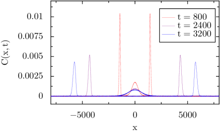
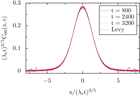
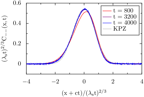
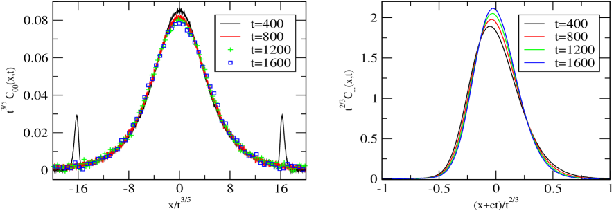
Set II: $k_{2}=1.0,k_{3}=2.0,k_{4}=1.0,T=5.0,P=1.0$. This choice of parameters gives $c=1.80293$ and we see in Fig. (4) there is much better separation of the heat and sound modes. We again find an excellent collapse of the heat mode and the sound mode data with the expecteded scalings Fig. (5) . The heat mode fits very well to the Lévy-scaling function. However the sound-mode scaling function still shows significant asymmetry and is different from the KPZ function. The theoretical obtained values of $\lambda_{s}=0.396$ and $\lambda_{e}=5.89$ are now close to the numerically estimated values $\lambda_{s}=0.46$ and $\lambda_{e}=5.86$.

Set III: $k_{2}=1.0,k_{3}=-1.0,k_{4}=1.0,T=0.1,P=0.07776$. Our third choice of the parameter set is motivated by recent nonequilibrium simulations zhao12 ; zhao13 which find that the thermal conductivity $\kappa$ at low temperatures seems to converge to a size-independent value, contradicting the expectation that heat conduction is anomalous and $\kappa$ should diverge with system size at all temperatures. It has been suggested that this could be a finite size effect das14 ; wang13 ; savin14 , but this has not been established convincingly yet. Here we want to explore if the equal-time correlations show any signatures of diffusive heat transport and if they provide any additional insight regarding the strong finite size effects seen in the nonequilibrium studies. The temperature chosen is $T=0.1$, which for the FPU potential parameters above correspond to the regime at which normal conduction has been proposed.

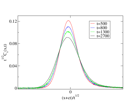
The speed of sound is calculated to be $c=1.09352$, which matches with the numerical data, as seen in Fig. (7). The heat mode seems to follow the predicted anomalous scaling reasonably well (though the convergence is, as expected, slower than in the high-temeprature case). We have checked that the same data, when scaled as $t^{1/2}C_{00}(x/t^{1/2})$ for different times, shows no indication of convergence. Thus we find no evidence for normal heat diffusion at low temperatures. The sound mode agrees quite well with the KPZ-type scaling observed for higher temperatures, though the shape of the correlation function remains asymmetric as in the high-temperature case.

It will be noted that the heat mode shows two peaks near the edges which do not follow the Lévy scaling - these peaks arise from interaction with the sound modes, indicating that there is still some overlap between the two modes near the edges. The sound mode, on the other hand, is found to be undistorted, which is consistent with the prediction from spohn13 that at long times the mode-coupling equations for the sound modes becomes independent of the heat mode, but not vice versa. the same effect can be seen in sets I and II, but are less pronounced as the heat and sounds separate more quickly at higher temperatures.

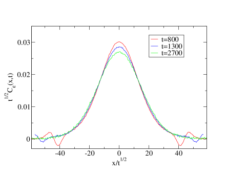
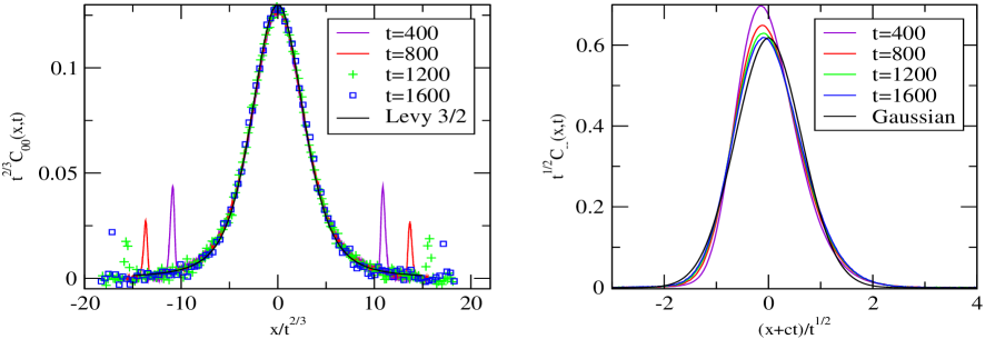
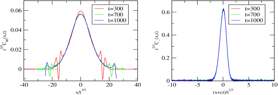
Set IV: $k_{2}=1.0,k_{3}=0.0,k_{4}=1.0,T=1.0,P=0.0$. This is the special case of an even potential at zero pressure for which the prediction from the theory is a diffusive sound mode, while the heat mode is Lévy but with a different exponent. The predicted scalings are given in Eqs. (8,9). The speed of sound for this case is $c=1.46189$. We see from Fig. (8) that the proposed scaling leads to an excellent collapse of the heat mode at different times. The sound mode, with diffusive scaling, shows a strong convergence but not yet a collapse. Fig. 9 shows the same data but scaled according to the predictions in the non-zero pressure case. It is clear that the data are non-convergent with this scaling.

The sound mode is predicted by the theory to be Gaussian, Eq. (8), but as seen from Fig. (8), the fit to the Gaussian form is poor. From the data we estimate that $\lambda_{s}^{0}=0.416$, and upon using Eq. (11), we find $\lambda_{e}^{0}=1.17$, whereas the numerically obtained value is $3.18$.

Set V: $k_{2}=1.0,k_{3}=0.0,k_{4}=1.0,T=1.0,P=1.0$ Parameters are identical to the above set, except that the pressure is non-zero. Since the potential is even, the pressure arises from externally applied stress to the system. The speed of sound is $c=1.59143$. We find in Fig. 10 that the correlations satisfy the same scaling as a generic asymmetric potentials with non-zero pressure (sets I, II, III). This confirms that the universality class is determined by the asymmetry of $V(r)+Pr$ and not of $V(r)$ by itself.

III Discussion

We have performed numerical simulations of FPU chains to test the predictions of nonlinear fluctuating hydrodynamics in one dimension spohn13 . The theory predicts the existence of a zero velocity heat mode and two mirror image moving sound modes, and provides their asymptotic scaling forms. We have tested the theory for various parameter regimes, including high and low temperatures, and zero and non-zero pressure regimes. For non-zero pressure, we find that the heat mode scales according to the Lévy-5/3 distribution, as predicted by the theory, both at high and low temperatures. This implies that for one-dimensional heat transport (in momentum-conserving systems) the scaling is generically anomalous. There are no signatures of a non-equilibrium phase transition (or crossover) from anomalous to normal conduction. For the case of an even potential at zero pressure, the heat mode scales according to the Lévy-3/2 distribution as predicted, thus confirming the existence of a second universality class for heat transport in one-dimensional momentum-conserving systems.

For non-zero pressure the sound mode spatio-temporally scales with the same exponents as the KPZ function, but the shape of the modes is observed not to have collapsed to the KPZ function. This could be because the simulation times are not in the asymptotic regime for the sound modes, which would be consistent with the slowly decaying correction terms to the scaling forms of the sound mode as discussed in spohn13 . Thus the prediction that the sound mode correlations scale according to the KPZ function is not conclusively verified. The case of an even potential at zero pressure is very similar, with the sound mode satisfying diffusive scaling, but the limit of the Gaussian scaling shape is not reached in our simulations.

Although the Lévy stable distribution fits the heat modes very well, we find that at low temperatures the theoretically predicted values for the scaling coefficients $\lambda_{s}$ and $\lambda_{e}$ do not well match the numerical values. This is consistent with the numerical study in mendl14 , where the authors find that for certain hard-point potentials the scaling shape has an excellent match, but the scaling coefficients are still drifting and one might hope them to converge to the predicted values at larger times. However at high temperatures where the modes are well-separated, the theoretical $\lambda_{e}$ matches very well with the numerical data, and the theoretical $\lambda_{s}$ is not far off from the numerically obtained value.

An open and important question is to tie up the picture obtained from the correlation dynamics in equilibrium studies with the nonequilibrium properties of FPU chains. The studies here confirm that heat conduction in one-dimensional chains is anomalous. We do not see any signatures of the apparent diffusive behavior (possibly related to finite size-effects) observed in nonequibrium studies at low temperatures zhao12 ; das14 ; wang13 . A clear microscopic understanding of the puzzling strong finite size-effects is lacking.

IV Acknowledgements

A.D thanks DST for support through the Swarnajayanti fellowship. K.S was supported by MEXT (25103003) and JSPS (90312983). We thank Manas Kulkarni for useful discussions.

V Appendix

The matrix $R$, which diagonalizes the matrix $A$, is given by

$$R=\sqrt{\frac{2\beta}{c^{2}}}\left(\begin{array}[]{ccc}\partial_{l}p&-c&\partial_{e}p\\ \widetilde{\kappa}p&0&\widetilde{\kappa}\\ \partial_{l}p&c&\partial_{e}p\end{array}\right),$$ (14)

where the columns, including the normalization factor, provide the right eigenvectors $V_{\alpha}$, $\alpha=-1,0,1$, of the $A$ matrix.

The Hessian tensor $H$ encodes the quadratic corrections to the couplings between the original hydrodynamic variables. $H^{\alpha}_{\beta\gamma}$ represents the coupling of the field component $\alpha$ to the field components $\beta$, $\gamma$. The tensor can be represented through three $3\times 3$ matrices, one for each value of $\alpha$,

$H^{u_{1}}=0$,  $H^{u}=\left(\begin{array}[]{ccc}\partial^{2}_{l}p&0&\partial_{l}\partial_{e}p\\ 0&-\partial_{e}p&0\\ \partial_{l}\partial_{e}p&0&\partial^{2}_{e}p\end{array}\right)$,  $H^{e}=\left(\begin{array}[]{ccc}0&\partial_{l}p&0\\ \partial_{l}p&0&\partial_{e}p\\ 0&\partial_{e}p&0\end{array}\right)$.

After transforming to the normal modes $\vec{\phi}$, the nonlinear hydrodynamic equations become

$$\partial_{t}\phi_{\alpha}=-\partial_{x}\left[c_{\alpha}\phi_{\alpha}+\langle\vec{\phi}.G^{\alpha}\vec{\phi}\rangle-\partial_{x}{(D\phi)}_{\alpha}+{(B\xi)}_{\alpha}\right]~{}.~{}~{}~{}~{}$$

The term in angular brackets is the inner product of $G^{\alpha}$ with respect to $\vec{\phi}$. Also, $D=R\widetilde{D}R^{-1}$ and $B=R\widetilde{B}$ satisfy the fluctuation-dissipation relation $BB^{T}=2D$. The vector $\vec{c}=(-c,0,c)$.

The tensor $G$ represents the coupling between the normal modes and is given by $G^{\alpha}=\frac{1}{2}\sum_{\alpha^{\prime}=1}^{3}R_{\alpha\alpha^{\prime}}(R^{-1})^{T}H^{\alpha^{\prime}}R^{-1}$. The the elements of $G^{\alpha}$ can be represented through cumulants of $V$, $r$ with respect to the single site distribution up to order three, see spohn13 .

The values of $R$ and $G^{0}$ and $G^{1}$ are given below. The elements of $G^{-1}$ are a rearrangement of the elements of $G^{1}$ as follows from $G^{-1}_{-\alpha~{}-\beta}=-G^{1}_{\alpha\beta}$,  $G^{-1}_{-10}=G^{-1}_{01}$ and $G^{-1}_{\alpha\beta}=G^{1}_{\beta\alpha}$ spohn13 . The long time behavior is dominated by the diagonal $G$ entries. The off-diagonal entries are irrelevant. $G^{s}_{ss}$ are the self-couplings. Note that $G^{0}_{00}=0$, as claimed before. Also for the even potential at zero pressure case the only leading terms are $G^{0}_{ss}$, $s=\pm 1$. There is considerable variation in the diagonal matrix elements.

Set I

$R=\left(\begin{array}[]{ccc}-0.7935&-1.&0.66118\\ 1.89594&0.0&1.89594\\ -0.7935&1.&0.66118\end{array}\right)$,   $G^{0}=\left(\begin{array}[]{ccc}-0.689497&0.0&0.0\\ 0.0&0.0&0.0\\ 0.0&0.0&0.689497\end{array}\right)$,  $G^{1}=\left(\begin{array}[]{ccc}-0.24236&-0.075565&.238543\\ -0.075565&-0.0669417&-0.075565\\ .238543&-0.075565&0.238543\end{array}\right).$

Set II

$R=\left(\begin{array}[]{ccc}-0.547157&-0.316228&0.0229798\\ 0.229483&0.0&0.229483\\ -0.547157&0.316228&0.0229798\end{array}\right)$,  $G^{0}=\left(\begin{array}[]{ccc}-1.03436&0.0&0.0\\ 0.0&0.0&0.0\\ 0.0&0.0&1.03436\end{array}\right)$,  $G^{1}=\left(\begin{array}[]{ccc}-.0671336&.240399&.140022\\ .240399&-.152971&.240399\\ .140022&.240399&.140022\end{array}\right).$

Set III

$R=\left(\begin{array}[]{ccc}-2.3376&-2.23607&1.38344\\ 0.793106&0.0&10.1994;\\ -2.3376&2.23607&1.38344\end{array}\right)$,  $G^{0}=\left(\begin{array}[]{ccc}-0.55766&0.0&0.0\\ 0.0&0.0&0.0\\ 0.0&0.0&0.55766\end{array}\right)$,  $G^{1}=\left(\begin{array}[]{ccc}-0.0721968&0.0206018&0.0790847\\ 0.0206018&-0.0353259&0.0206018\\ 0.0790847&0.0206018&0.0790847\end{array}\right).$

Set IV

$R=\left(\begin{array}[]{ccc}-1.03371&-0.707107&0.0\\ 0.0&0.0&1.09893\\ -1.03371&0.707107&0.0\end{array}\right)$,  $G^{0}=\left(\begin{array}[]{ccc}-0.803254&0.0&0.0\\ 0.0&0.0&0.0\\ 0.0&0.0&0.803254\end{array}\right)$,  $G^{1}=\left(\begin{array}[]{ccc}0.0&0.133622&0.0\\ 0.133622&0.0&.133622\\ 0.0&.133622&0.0\end{array}\right)$.

Set V

$R=\left(\begin{array}[]{ccc}-0.964170&-0.707106&-0.964171\\ 1.05385&0.0&1.05385584\\ 0.161141&0.707107&0.161141\end{array}\right)$,  $G^{0}=\left(\begin{array}[]{ccc}-0.838569&0.0&0.0\\ 0.0&0.0&0.0\\ 0&0&0.838569\end{array}\right)$,  $G^{1}=\left(\begin{array}[]{ccc}-0.112782&0.07359&0.143663\\ 0.07359&-0.104607&0.07359\\ 0.143663&0.07359&0.143663\end{array}\right)$.

References

- (1) S. Lepri, R. Livi, and A. Politi, Phys. Rep. 377, 1 (2003).
- (2) A. Dhar, Adv. Phys. 57, 457 (2008).
- (3) S. Lepri, R. Livi, and A. Politi, Phys. Rev. Lett. 78, 1896 (1997).
- (4) A. Dhar, Phys. Rev. Lett. 88, 249401 (2002).
- (5) P. Grassberger, W. Nadler, and L. Yang, Phys. Rev. Lett. 89, 180601 (2002).
- (6) G. Casati and T. Prosen, Phys. Rev. E 67, 015203 (2003).
- (7) T. Mai, A. Dhar and O. Narayan, Phys. Rev. Lett. 98, 184301 (2007).
- (8) L. Delfini, S. Lepri, R. Livi, A. Politi, Phys. Rev. E 73, 060201 (2006).
- (9) O. Narayan and S. Ramaswamy, Phys. Rev. Lett. 89, 200601 (2002).
- (10) J. S. Wang and B. Li, Phys. Rev. Lett. 92, 074302 (2004).
- (11) A. Pereverzev, Phys. Rev. E 68 056124 (2003).
- (12) J. Lukkarinen and H. Spohn, Commun. Pure Appl. Math. 61 1753-1786 (2008).
- (13) G. Basile, C. Bernardin and S. Olla, Phys. Rev. Lett.,96 204303 (2006).
- (14) H. van Beijeren, Phys. Rev. Lett. 108 , 180601 (2012).
- (15) J. M. Deutsch and O. Narayan, Phys. Rev. E 68, 041203 (2003).
- (16) H. Zhao, Phys. Rev. Lett. 96 140602 (2006).
- (17) S. Chen, Y. Zhang, J. Wang and H. Zhao, arXiv:1106.2896v2 (2011).
- (18) P. Cipriani, S. Denisov, and A. Politi, Phys. Rev. Lett. 94, 244301 (2005).
- (19) V. Zaburdaev, S. Denisov, and P. Hänggi, Phys. Rev. Lett. 106, 180601 (2011).
- (20) S. Lepri and A. Politi, Phys. Rev. E 83 030107 (2011).
- (21) A. Dhar, K. Saito and B. Derrida Phys. Rev. E 87, 010103(R) (2013).
- (22) S. Liu, P. Hänggi, N. Li, J. Ren and B. Li, Phys. Rev. Lett. 112, 040601 (2014).
- (23) C. B. Mendl, H. Spohn, Phys. Rev. Lett. 111, 230601 (2013).
- (24) H. Spohn, J. Stat. Phys. 154, 1191 (2014).
- (25) C. B. Mendl, H. Spohn, arXiv:1403.0213 (2014).
- (26) G. P. Berman and F. M. Izrailev in “The Fermi–Pasta–Ulam problem: Fifty years of progress”, Chaos 15, 015104 (2005).
- (27) G. Benettin, A. Ponno, J. Stat. Phys. 144, 793 (2011).
- (28) H. Kantz, R. Livi, S. Ruffo, J. Stat. Phys. 76, 627 (1994).
- (29) M. Prähofer, H. Spohn, J. Stat. Phys. 115, 255 (2004)
- (30) M. Prähofer, http://www-m5.ma.tum.de/KPZ.
- (31) M. Jara, T. Komorowski, and S. Olla, arXiv:1402.2988
- (32) M. P. Allen and D. L. Tildesley, Computer Simulations of Liquids (Clarendon, Oxford, 1987).
- (33) Y. Zhong, Y. Zhang, J. Wang, H. Zhao, Phys. Rev. E 85, 060102(R) (2012).
- (34) S. Chen, Y. Zhang, J. Wang, H. Zhao, arXiv:1204.5933.
- (35) S. G. Das, A. Dhar, O. Narayan, J. Stat. Phys. 154, 204 (2014).
- (36) L. Wang, B. Hu and B. Li, Phys. Rev. E 88, 052112 (2013).
- (37) A.V. Savin and Y. A Kosevich, Phys. Rev. E 89, 032102 (2014).