Abstract

The ratio between two probability density functions is an important component of various tasks, including selection bias correction, novelty detection and classification. Recently, several estimators of this ratio have been proposed. Most of these methods fail if the sample space is high-dimensional, and hence require a dimension reduction step, the result of which can be a significant loss of information. Here we propose a simple-to-implement, fully nonparametric density ratio estimator that expands the ratio in terms of the eigenfunctions of a kernel-based operator; these functions reflect the underlying geometry of the data (e.g., submanifold structure), often leading to better estimates without an explicit dimension reduction step. We show how our general framework can be extended to address another important problem, the estimation of a likelihood function in situations where that function cannot be well-approximated by an analytical form. One is often faced with this situation when performing statistical inference with data from the sciences, due the complexity of the data and of the processes that generated those data. We emphasize applications where using existing likelihood-free methods of inference would be challenging due to the high dimensionality of the sample space, but where our spectral series method yields a reasonable estimate of the likelihood function. We provide theoretical guarantees and illustrate the effectiveness of our proposed method with numerical experiments.

1 INTRODUCTION

There has been growing interest in the problem of estimating the ratio of two probability densities, $\beta({\mathbf{x}})\equiv f({\mathbf{x}})/g({\mathbf{x}})$, given $i.i.d.$ samples from unknown distributions $F$ and $G$. For example, these ratios play a key role in matching training and test data in so-called transfer learning or domain adaptation (Sugiyama et al., 2010a), where the goal is to predict an outcome $y$ given test data ${\mathbf{x}}$ from a distribution ($G$) that is different from that of the training data ($F$). Estimated density ratios also appear in novelty detection (Hido et al., 2011), conditional density estimation (Sugiyama et al., 2010b), selection bias correction (Gretton et al., 2010), and classification (Nam et al., 2012).

Experiments have shown that it is suboptimal to estimate $\beta({\mathbf{x}})$ by first estimating the two component densities and then taking their ratio (Sugiyama et al., 2008). Hence, several alternative approaches have been proposed that directly estimate $\beta({\mathbf{x}})$; e.g., uLSIF, an estimator obtained via least-squares minimization (Kanamori et al., 2009); KLIEP, which is obtained via Kullback-Leibler divergence minimization (Sugiyama et al., 2008); KuLSIF, a kernelized version of uLSIF (Kanamori et al., 2012); and kernel mean matching, which is based on minimizing the mean discrepancy between transformations of the two samples in a Reproducing Kernel Hilbert Space (RKHS) (Gretton et al., 2010). For a review of techniques see Margolis (2011).

Existing methods are not effective when ${\mathbf{x}}$ is of high dimension, and hence authors recommend a dimension reduction prior to implementation (Sugiyama et al., 2011). As is the case with any data reduction, such a step can result in significant loss of information. Here we propose a novel series estimator of $\beta({\mathbf{x}})$ designed to take advantage of the intrinsic dimensionality of ${\mathbf{x}}$, but without an explicit dimension reduction step. Thus, this work addresses a critical need by constructing a nonparametric estimator for $\beta({\mathbf{x}})$ which performs well even when ${\mathbf{x}}$ is of high dimension.

Our method is fast and simple to implement. To approximate $\beta({\mathbf{x}})$, we expand $\beta$ in terms of the eigenfunctions of a kernel-based operator. These eigenfunctions are orthogonal with respect to the underlying data distribution as opposed to the Lebesgue measure on the ambient space. In fact, the eigenfunctions form a Fourier-like basis adapted to the submanifold structure with the low-order components smoother than the higher-order ones, see Figure 1. As we shall see, this basis is particularly well-suited for approximating smooth functions in high dimensions. Unlike RKHS methods (Gretton et al., 2010) (which do not explicitly compute the eigenfunctions themselves), our approach to nonparametric density estimation allows for out-of-sample extensions and a principled way of choosing tuning parameters via well-studied model selection techniques such as cross-validation.

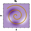
Figure 1: Level sets of the top three eigenfunctions of a kernel-based operator when the support of the data $(x,y)$ is close to a spiral. The eigenfunctions form a Fourier-like basis adapted to the geometry of the data. This basis is well-suited for approximating smooth functions in the region around the spiral.

We extend our proposed methodology for estimating density ratios to the problem of estimating the likelihood function of observing data ${\mathbf{x}}$ given parameters $\theta$. Estimation of the likelihood is necessary when the complexity of the data-generation process prevents derivation of a sufficiently accurate analytical form for the likelihood function. Here we exploit the fact that, in many such situations, one can simulate data sets ${\mathbf{x}}$ under different parameters $\theta$. This is often the case in statistical inference problems in the sciences, where the relationship between parameters of interest and observable data is complex, but accurate simulation models are available; see, for example, genetics (Beaumont 2010; Estoup et al. 2012) and astronomy (Cameron and Pettitt 2012; Weyant et al. 2013). Problems of this type have motivated recent interest in methods of likelihood-free inference, which includes methods of Approximate Bayesian Computation (ABC); see Marin et al. (2012) for a review.

In our implementation, we redefine the likelihood function as ${\mathcal{L}}({\mathbf{x}};\theta)\equiv f({\mathbf{x}}|\theta)/g({\mathbf{x}})$, where $g({\mathbf{x}})$ is a density with support larger than that of $f({\mathbf{x}}|\theta)$. This formulation differs from the standard definition of the likelihood by only a multiplicative term which is constant in $\theta$, and hence ${\mathcal{L}}({\mathbf{x}};\theta)$ can still be used for likelihood-based inference (including maximum likelihood estimation). In particular, the shape of the posterior for $\theta$ is unaffected. The challenge of estimating the likelihood is now a density ratio estimation problem. This approach will yield significant advantages in cases where $g$ is chosen to focus high probability on the low-dimensional subspace in which the data ${\mathbf{x}}$ lie. One natural choice is $g({\mathbf{x}})=\int f({\mathbf{x}}|\theta)d\pi(\theta)$, where $\pi$ is a well-chosen prior distribution for $\theta$. The orthogonality of the spectral series with respect to $g$ results in an efficient implementation of the estimator. Moreover, directly estimating the ratio $f({\mathbf{x}}|\theta)/g({\mathbf{x}})$ may itself be easier than estimating $f({\mathbf{x}}|\theta)$, e.g., when the conditional distributions $f({\mathbf{x}}|\theta)$ for different $\theta$ are similar, or when they have similar support in high dimensions. To our knowledge, this is the first work that proposes a spectral series approach to non-parametric density estimation and likelihood inference in high dimensions.

The organization of the paper is as follows: In Section 2 we present our density ratio estimator and apply it to a prediction problem in astronomy with covariate shift. In Section 3, we show how our method can be extended to estimating a likelihood function, and provide experiments that show its advantages over traditional methods. Finally, in Section 4, we provide theoretical guarantees and rates of convergence of the proposed estimators. Full proofs as well as details on the astronomy data are provided in Supplementary Materials.

2 SPECTRAL SERIES ESTIMATOR OF A DENSITY RATIO

In this section we will present the mathematical details behind our spectral series estimator of a density ratio. To begin, let $\mathbf{x}$ denote a $d$-dimensional random vector, assumed to lie in the subspace $\mathcal{X}$. We observe an $i.i.d.$ sample $\mathbf{x}^{F}_{1},\ldots,\mathbf{x}^{F}_{n_{F}}$ from an unknown distribution $F$, as well as an $i.i.d.$ sample $\mathbf{x}^{G}_{1},\ldots,\mathbf{x}^{G}_{n_{G}}$ from an unknown distribution $G$. The goal is to estimate

$$\beta(\mathbf{x})\equiv f({\mathbf{x}})/g({\mathbf{x}}).$$

We assume that $F\ll G$ so that this ratio is well-defined.

Let $K_{\mathbf{x}}(\mathbf{z},\mathbf{y})$ be a bounded, symmetric, and positive definite kernel, and let $\{\psi_{j}\}_{j\in\mathbb{N}}$ be the eigenfunctions of the operator $\textbf{K}_{\mathbf{x}}:L^{2}(\mathcal{X},G)\longrightarrow L^{2}(\mathcal{X},G)$ (Rosasco et al., 2010):

$$\textbf{K}_{\mathbf{x}}(h)(\mathbf{z})=\int_{\mathcal{X}}K_{\mathbf{x}}(\mathbf{z},\mathbf{y})h(\mathbf{y})dG(\mathbf{y}).$$ (1)

Our spectral series estimator relies on the fact that $\{\psi_{j}\}_{j\in\mathbb{N}}$ is an orthonormal basis of $L^{2}(\mathcal{X},G)$, i.e., the eigenfunctions are orthonormal with respect to the data distribution $G$ rather than the Lebesgue measure:

$$\int_{\mathcal{X}}\psi_{i}(\mathbf{x})\psi_{j}(\mathbf{x})dG(\mathbf{x})={\mathbb{I}}(i=j).$$

Hence, for $\beta(\mathbf{x})\in L^{2}(\mathcal{X},G)$, we can write

$$\beta(\mathbf{x})=\sum_{j\in\mathbb{N}}\beta_{j}\psi_{j}(\mathbf{x}),$$ (2)

where $\beta_{j}=\int\beta(\mathbf{x})\psi_{j}(\mathbf{x})dG(\mathbf{x})={\mathbb{E}}_{F}[\psi_{j}(\mathbf{X})].$

Since $G$ is unknown, the $\psi_{j}$’s must be estimated. First, we compute the $J\leq n_{G}$ eigenvectors $\widetilde{\psi}_{1},\ldots,\widetilde{\psi}_{J}$ (with largest eigenvalues) of the Gram matrix based on the sample from $G$,

$$\left[K_{\mathbf{x}}\left(\mathbf{x}^{G}_{i},\mathbf{x}^{G}_{j}\right)\right]_{i,j=1}^{n_{G}}.$$

These functions are then extended to all ${\mathbf{x}}\in\mathcal{X}$ via the Nyström Extension (Drineas and Mahoney, 2005)

$$\widehat{\psi}_{j}(\mathbf{x})=\frac{\sqrt{n_{G}}}{\widehat{\ell}^{{\mathbf{x}}}_{j}}\sum_{k=1}^{n_{G}}\widetilde{\psi}_{j}\left(\mathbf{x}^{G}_{k}\right)K_{\mathbf{x}}\left(\mathbf{x},\mathbf{x}^{G}_{k}\right),$$

where $\widehat{\ell}^{{\mathbf{x}}}_{j}$ is the eigenvalue associated to the eigenvector $\widetilde{\psi}_{j}$. Next we estimate the $\beta_{j}$’s in Eq. (2) using the sample from $F$:

$$\widehat{\beta}_{j}=\frac{1}{n_{F}}\sum_{k=1}^{n_{F}}\widehat{\psi}_{j}\left(\mathbf{x}^{F}_{k}\right).$$

Our spectral series estimator is finally given by

$$\widehat{\beta}({\mathbf{x}})=\left(\sum_{j=1}^{J}\widehat{\beta}_{j}\widehat{\psi}_{j}({\mathbf{x}})\right)_{\!+}.$$ (3)

This approach can be motivated as follows. The basis functions $\widehat{\psi}_{j}$ are consistent estimators of the eigenfunctions $\psi_{j}$ of the corresponding integral operator (Bengio et al., 2004). In our nonparametric model, $J$ is a tuning parameter that controls the bias/variance tradeoff: Decreasing $J$ decreases the variance, but increases the bias of the estimator. We choose $J$ (and the other tuning parameters) in a principled way described below.

Model Selection. To evaluate the performance of an estimator $\widehat{\beta}({\mathbf{x}})$, we use the loss function

$$L(\widehat{\beta},\beta) \equiv\int\left(\widehat{\beta}(\mathbf{x})-\beta(\mathbf{x})\right)^{2}dG(\mathbf{x})$$

$$=\int\widehat{\beta}(\mathbf{x})^{2}dG(\mathbf{x})-2\!\int\widehat{\beta}(\mathbf{x})dF(\mathbf{x})+K$$

where $K$ does not depend on $\widehat{\beta}$. We estimate this quantity (up to $K$) using

$$\widehat{L}(\widehat{\beta},\beta)=\frac{1}{\widetilde{n}_{G}}\sum_{k=1}^{\widetilde{n}_{G}}\widehat{\beta}^{2}(\widetilde{\mathbf{x}}_{k}^{G})-\frac{2}{\widetilde{n}_{F}}\sum_{k=1}^{\widetilde{n}_{F}}\widehat{\beta}(\widetilde{\mathbf{x}}_{k}^{F}),$$ (4)

where $\widetilde{{\mathbf{x}}}^{G}_{1},\ldots,\widetilde{{\mathbf{x}}}^{G}_{\widetilde{n}_{G}}$ is a validation sample from $G$, and $\widetilde{{\mathbf{x}}}^{F}_{1},\ldots,\widetilde{{\mathbf{x}}}^{F}_{\widetilde{n}_{F}}$ is a validation sample from $F$. Tuning parameters are chosen to minimize $\widehat{L}(\widehat{\beta},\beta)$. Note that because of the orthogonality of the $\widehat{\psi}_{j}$, it is not necessary to recompute the estimated coefficients $\widehat{\beta}_{j}$’s for each value of $J$ in Eq. (3), unlike most estimation procedures, where estimated coefficients have to be recomputed for each configuration of the tuning parameters. In other words, only the tuning parameters associated with the kernel (in our case, the kernel bandwidth $\epsilon$) affect the computation time.

2.1 Application: Correction to Covariate Shift in Photometric Redshift Prediction

Assume we observe a sample of unlabeled data, as well as a sample of labeled data, where the $Z$’s represent the labels and $\mathbf{x}$’s are the covariates. One is often interested in estimating the regression function ${\mathbb{E}}[Z|\mathbf{x}]$ under selection bias, i.e., in situations where the distributions of labeled and unlabeled samples ($f_{L}({\mathbf{x}})$ and $f_{U}({\mathbf{x}})$, respectively) are different. If the estimate $\widehat{{\mathbb{E}}}[Z|\mathbf{x}]$ is constructed using the labeled data with the goal of predicting $Z$ from $\mathbf{x}$ on the unlabeled data, corrections have to be made. A key quantity for making this correction under the covariate shift assumption (Shimodaira, 2000) is the density ratio $f_{U}({\mathbf{x}})/f_{L}({\mathbf{x}})$, the so-called importance weights (Gretton et al., 2010). We now compare various estimators of importance weights for a key problem in astronomy, namely that of redshift estimation (Sheldon et al., 2012).

Figure 2: Estimated losses of $\widehat{\beta}({\mathbf{x}})$ with standard errors for SDSS data. The spectral series estimator has best performance.

We use a subset of the Sloan Digital Sky Survey (Aihara et al., 2011). The ultimate goal is to build a predictor of galaxy redshift $Z$ based on photometric data ${\mathbf{x}}$; see Supplementary Materials for details. We are given a training set with covariates ${\mathbf{x}}$ of galaxies and their redshifts, as well as unlabeled target data. Because it is difficult to acquire the true redshift of faint galaxies, these data suffer from selection bias. We compare our method of estimating the importance weights (Series) to uLSIF, KLIEP, and KuLSIF, described in Section 1. We also compute LHSS, which uses uLSIF after applying a dimension reduction technique specifically designed for estimating a density ratio, see Sugiyama et al. (2011). Moreover, we include a comparison with a $k$-nearest neighbors estimator (KNN) proposed in the astronomy literature (Lima et al. 2008), which it not based on ratios. We do not show results of ratio-based estimators because the estimates of $f_{L}({\mathbf{x}})$ are close to zero for many ${\mathbf{x}}$’s, inducing estimates of $\beta$ that are infinity.

Figure 2 shows the estimated losses of the different methods of estimating the ratio $f_{U}({\mathbf{x}})/f_{L}({\mathbf{x}})$ when using 5,000 labeled and 5,000 unlabeled samples, and 10 photometric covariates ${\mathbf{x}}$. We use 60% of the data for training, 20% for validation and 20% for testing. Even though this example has a covariate space with as few as 10 dimensions, we can already see the benefits of the spectral series estimator.

3 EXTENSION: SPECTRAL SERIES ESTIMATOR OF A LIKELIHOOD FUNCTION

Our framework for estimating density ratios can be extended to the problem of estimating a high-dimensional likelihood function. To the derivation described above, we add $\theta\in\Theta$, the $p$-dimensional parameter. In this context, ${\mathbf{x}}\in\mathcal{X}\subseteq\Re^{d}$ is a random vector representing a single sample observation. We will adopt a Bayesian perspective, and let $F_{\theta}$ be the marginal distribution for $\theta$, i.e., the prior, and let $G$ denote the marginal distribution for ${\mathbf{x}}$. Then, let $({\mathbf{x}}_{1}^{F},\theta_{1}),\ldots,({\mathbf{x}}_{n_{F}}^{F},\theta_{n_{F}})$ be an $i.i.d.$ sample from the joint distribution of ${\mathbf{x}}$ and $\theta$. Further, let $\mathbf{x}^{G}_{1},\ldots,\mathbf{x}^{G}_{n_{G}}$ be an $i.i.d.$ sample from $G$. Our objective is to estimate the ratio

$${\mathcal{L}}({\mathbf{x}};\theta)\equiv\frac{f({\mathbf{x}}|\theta)}{g({\mathbf{x}})},$$ (5)

where $f({\mathbf{x}}|\theta)$ is the conditional density of ${\mathbf{x}}$ given $\theta$, and $g({\mathbf{x}})$ is the marginal density for ${\mathbf{x}}$. This is, up to a multiplicative factor that is not a function of $\theta$, the standard definition of the likelihood function.

To estimate ${\mathcal{L}}(x;\theta)$, we use a spectral series approach as before, but because the likelihood is a function of both ${\mathbf{x}}$ and $\theta$, we consider the tensor product of a basis for ${\mathbf{x}}$ and a basis for $\theta$, $\{\Psi_{i,j}\}_{i,j\in\mathbb{N}}$, where

$$\Psi_{i,j}({\mathbf{x}},\theta)=\psi_{j}(\mathbf{x})\phi_{i}(\theta),\ i,j\in\mathbb{N}.$$

The construction of the separate bases $\{\psi_{j}\}_{j}$ and $\{\phi_{i}\}_{i}$ proceeds just as described in Section 2. Note that for $\theta$, we consider the eigenfunctions $\{\phi_{i}\}_{i}$ of the operator $\textbf{K}_{\theta}\!:L^{2}(\Theta,F_{\theta})\longrightarrow L^{2}(\Theta,F_{\theta})$:

$$\textbf{K}_{\theta}(h)(\xi)=\int_{\Theta}K_{\theta}(\xi,\mu)h(\mu)dF_{\theta}(\mu),$$

where $K_{\theta}$ is not necessarily the same kernel as $K_{{\mathbf{x}}}$. That is, while $\{\psi_{j}\}_{j}$ is estimated using a Gram matrix based on $\mathbf{x}^{G}_{1},\ldots,\mathbf{x}^{G}_{n_{G}}$, $\{\phi_{i}\}_{i}$ is estimated using $\theta_{1},\ldots,\theta_{n_{F}}$.

Since $\{\phi_{i}\}_{i}$ is an orthonormal basis of functions in $L^{2}(\Theta,F_{\theta})$, the tensor product $\{\Psi_{i,j}\}_{i,j}$ is an orthonormal basis for functions in $L^{2}(\Theta\times\mathcal{X},F_{\theta}\times G)$.

The projection of ${\mathcal{L}}({\mathbf{x}};\theta)$ onto $\{\Psi_{i,j}\}_{i,j}$ is given by

$$\sum_{i,j\in\mathbb{N}}\beta_{i,j}\Psi_{i,j}({\mathbf{x}},\theta),$$

where

$$\beta_{i,j} =\iint{\mathcal{L}}({\mathbf{x}};\theta)\Psi_{i,j}({\mathbf{x}},\theta)dG({\mathbf{x}})dF_{\theta}(\theta)$$

$$={\mathbb{E}}_{F}\!\left[\Psi_{i,j}({\mathbf{x}},\theta)\right].$$ (6)

Hence, we define our likelihood function estimator by

$$\widehat{{\mathcal{L}}}({\mathbf{x}};\theta)=\sum_{i=1}^{I}\sum_{j=1}^{J}\widehat{\beta}_{i,j}\widehat{\Psi}_{i,j}({\mathbf{x}},\theta),$$

where $\widehat{\beta}_{i,j}=\frac{1}{n_{F}}\sum_{k=1}^{n_{F}}\widehat{\Psi}_{i,j}\left(\mathbf{x}^{F}_{k},\theta_{k}\right)$, and

$$\widehat{\Psi}_{i,j}({\mathbf{x}},\theta)=\widehat{\psi}_{j}(\mathbf{x})\widehat{\phi}_{i}(\theta)$$

is the estimator for $\Psi_{i,j}({\mathbf{x}},\theta)$, obtained via a Nyström extension as in Section 2. The tuning parameters $I$ and $J$ control the bias/variance tradeoff. Because we define the likelihood in terms of $g({\mathbf{x}})$ (Eq. 5), we can take advantage of the orthogonality of the basis functions when estimating the coefficients $\beta_{i,j}$; see Eq. 3. The result is a simple and fast-to-implement procedure for estimating likelihood functions for high-dimensional data.

Model Selection. To evaluate the performance of a given estimator, we use the loss function

$$L\left(\widehat{{\mathcal{L}}},{\mathcal{L}}\right) \equiv \int\left(\widehat{{\mathcal{L}}}(\mathbf{x};\theta)-{\mathcal{L}}(\mathbf{x};\theta)\right)^{2}dG(\mathbf{x})dF(\theta)=$$ (7)

$$= \int\widehat{{\mathcal{L}}}(\mathbf{x};\theta)^{2}dG(\mathbf{x})dF(\theta)-$$

$$- 2\!\int\widehat{{\mathcal{L}}}(\mathbf{x};\theta)dF(\theta,\mathbf{x})+K,$$

where $K$ does not depend on $\widehat{{\mathcal{L}}}$. We can estimate this quantity (up to $K$) by

$$\widehat{L}\left(\widehat{{\mathcal{L}}},{\mathcal{L}}\right)= \frac{1}{B}\sum_{l=1}^{B}\left[\frac{1}{\widetilde{n}}\sum_{k=1}^{\widetilde{n}}\left(\widehat{{\mathcal{L}}}\left(\widetilde{{\mathbf{x}}}^{G}_{k}|\widetilde{\theta}^{(l)}_{k}\right)\right)^{2}\right]$$

$$-\frac{2}{\widetilde{n}}\sum_{k=1}^{\widetilde{n}}\widehat{{\mathcal{L}}}(\widetilde{\mathbf{x}}_{k}^{F}|\widetilde{\theta}_{k}),$$

where $\widetilde{{\mathbf{x}}}^{G}_{1},\ldots,\widetilde{{\mathbf{x}}}^{G}_{\widetilde{n}}$ is a validation sample from $G$; $(\widetilde{\theta}_{1},\widetilde{{\mathbf{x}}}^{F}_{1}),\ldots,(\widetilde{\theta}_{\widetilde{n}},\widetilde{{\mathbf{x}}}^{F}_{\widetilde{n}})$ is a validation sample from the joint distribution of ${\mathbf{x}}$ and $\theta$; $\widetilde{\theta}_{1}^{(l)},\ldots,\widetilde{\theta}_{\widetilde{n}}^{(l)}$ for $l=1,\ldots,B$ are random permutations of the original sample $\widetilde{\theta}_{1},\ldots,\widetilde{\theta}_{\widetilde{n}}$; and $B$ is a number limited only by computational considerations. We choose tuning parameters so as to minimize $\widehat{L}$.

Remarks. By choosing an appropriate kernel, the spectral series approach can be extended to discrete data. For example, in Lee et al. (2010), p. 185, the authors suggest a distance kernel that take into account the discrete nature of genetic SNP data. By minimizing the loss in Eq. (7), one can also select the best kernel from a set of reasonable candidate kernels. Finally, our procedure can be scaled up to large sets of simulated data by speeding up the eigendecomposition of the Gram matrix. Possible methods include the Nyström extension (Drineas and Mahoney, 2005) and procedures described in, e.g., Belabbas and Wolfe (2009) and Halko et al. (2011). In particular, some of these approaches can be parallelized for even higher computational efficiency.

3.1 Numerical Experiments

Estimation of a likelihood function is of particular value in cases where the complexity of the data and the data-generating process prevents construction of a sufficiently accurate analytical form, a situation typically present in high-dimensional scientific data. The general setup is as follows. We have data which are modeled as an $i.i.d$. sample ${\mathbf{x}}_{1},\ldots,{\mathbf{x}}_{m}$ from the distribution $f({\mathbf{x}}|\theta)$. Our goal is to infer the value $\theta$. Although we are able to simulate from $f({\mathbf{x}}|\theta)$ for fixed $\theta$, we lack an analytical form for the likelihood function. Hence, we use the methodology of Section 3 to estimate ${\mathcal{L}}({\mathbf{x}};\theta)$ from a simulated sample. Once we have an estimate $\widehat{{\mathcal{L}}}({\mathbf{x}};\theta)$, we can approximate the likelihood of an observed sample according to

$$\widehat{{\mathcal{L}}}\left(({\mathbf{x}}_{1},\ldots,{\mathbf{x}}_{m});\theta\right)=\prod_{k=1}^{m}\widehat{{\mathcal{L}}}({\mathbf{x}}_{i};\theta).$$

This approximation can then be used in likelihood-based inference by, for example, plugging the expression into Bayes Theorem or by finding the maximum likelihood estimate.

In what follows we present five numerical examples where the ambient dimensionality of $\mathbf{x}$ is larger than its intrinsic dimensionality. In all experiments, we choose a uniform prior distribution on the parameter space.

Spiral. The data are $i.i.d.$ observations of $(X^{(1)},X^{(2)})$, where

$$X^{(1)}=\theta\cos{\theta}+N(0,1)\mbox{ and }X^{(2)}=\theta\sin{\theta}+N(0,1)$$

for $0<\theta<15$. Although the dimension of the sample space is 2, the data lie close to a one-dimensional spiral.

Klein Bottle. The data are $i.i.d.$ observations of $(X^{(1)},X^{(2)},X^{(3)},X^{(4)})$, where

$$\left\{\begin{array}[]{l}X^{(1)}=2(\cos{\theta_{2}}+1)\cos{\theta_{1}}+N(0,1)\\ X^{(2)}=2(\cos{\theta_{2}}+1)\sin{\theta_{1}}+N(0,1)\\ X^{(3)}=2\sin{\theta_{2}}\cos{\theta_{1}/2}+N(0,1)\\ X^{(4)}=2\sin{\theta_{2}}\sin{\theta_{1}/2}+N(0,1)\end{array}\right.$$

for $0<\theta_{1},\theta_{2}<2\pi$. The dimension of the sample is 4, but the data lie close to a two-dimensional Klein Bottle embedded in $\Re^{4}$.

Transformed Images. In this example, we rotate and translate an image of a tiger, see the top row of Figure 3. The model parameters are $(\theta,\rho_{x},\rho_{y})$. The transformed images are centered at $(\rho_{x}+N_{T}(0,10),\rho_{y}+N_{T}(0,10))$ with rotation angle $(\theta+N(0,10))$. The final images are cropped to $20\times 20$ pixels, i.e., the sample space has dimension $400$.

Transformed Images

Edges

Galaxies

Figure 3: Some examples of data generated according to Section 3.1. (The top left image is the original image in “Transformed Images”.)

Edges. Here we generate $20\times 20$ images of binary edges from a model with two parameters, $\alpha$ and $\lambda$. The data are $i.i.d.$ observations of an edge with rotation angle $\alpha+N(0,\pi/4)$ and displacement $\lambda+N_{T}(0,0.5)$ from the center, see Figure 3 for some examples.

Simulated Galaxy Images. The last example is a simplified version of a key estimation problem in astronomy, namely that of shear estimation (Bridle et al., 2009). We use the GalSim Toolkit to simulate realistic galaxy images. We sample two parameters: First, the orientation with respect to the $x$-axis of the image and, second, the axis ratio of the galaxies, which measures their ellipticity. To mimic a realistic situation, the observed data are low-resolution images of size $20\times 20$. Figure 3, bottom, shows some examples. These images have been degraded by observational effects such as background noise, pixelization, and blurring due to the atmosphere and telescope; see the Supplementary Materials for details.

We assume that the orientation and axis ratio of galaxy $i$ are given by $a_{i}\sim\mbox{Laplace}(\alpha,10)\mbox{ and }r_{i}\sim N_{T}(\rho,0.1^{2}),$ respectively. We seek to infer $\theta=(\alpha,\rho)$ based on an observed $i.i.d.$ sample of images ${\mathbf{x}}$ contaminated by observational effects. Notice we do not observe $a_{i}$ and $r_{i}$, but only $\mathbf{x}_{i}$, the 400-dimensional noisy image.

Methods. In the examples above, the likelihood function is estimated based on $n_{F}=n_{G}=5,000$ observations from the simulation model; 60% of the data are used for training and 40% for validation. We compare Series, our spectral series estimator from Section 3, with two state-of-the-art estimators of $f(\mathbf{x}|\theta)$. The first estimator is KDE – a kernel density estimator based on taking the ratio of kernel estimates of $f(\mathbf{x},\theta)$ and $f(\theta)$. We use the implementation from the package “np” (Hayfield and Racine, 2008) for R. For the Spiral and Klein bottle examples, we select the bandwidths of KDE via cross-validation. However, the high dimension of the other examples (Transformed, Edges, and Galaxy) makes a cross-validation approach computationally intractable and the density estimates numerically unstable. For these examples, we instead use the default reference rule for the bandwidth, and we reduce the dimensionality of the data with PCA with number of components chosen by minimizing the estimated loss (Eq. 7). The second estimator in our comparisons is LS – the direct least-squares conditional density estimator of Sugiyama et al. (2010b). This estimator is based on a direct expansion of the likelihood into a set of prespecified functions. This approach typically yields better results than estimators based on the ratio of random variables. Again, to avoid the problem of high dimensionality in the examples with $d>4$, we implement PCA+LS, the direct least-squares conditional density estimator after dimension reduction via PCA, with number of components chosen so as to minimize the estimated loss. PCA has the additional goal of decorrelating adjacent pixels in the images examples.

Table 1: Estimated $L^{2}$ loss (with standard errors) of the likelihood function estimators. Best-performing models with smallest loss are in bold fonts.

DATA	DIM.	$\mathbf{L^{2}}$ LOSS
		Series	LS	PCA+LS	KDE	PCA+KDE
Spiral	2	7.13 (0.14)	6.61 (0.12)	—	2.95 (0.30)	—
Klein Bottle	4	1.45 (0.07)	2.02 (0.06)	—	1.68 (0.11)	—
Transf. Images	400	20.94 (0.03)	26.91 (0.04)	27.12 (0.03)	—	26.62 (0.06)
Edges	400	0.70 (0.03)	1.77 (0.02)	1.55 (0.03)	—	1.60(0.02)
Galaxy Images	400	40.94 (0.03)	42.57 (0.01)	42.53 (0.01)	—	43.99 (0.04)

Table 2: Estimated average likelihood (with standard errors) of the likelihood function estimators. Best-performing models with largest average likelihood are in bold fonts.

DATA	DIM.	AVERAGE LIKELIHOOD
		Series	LS	PCA+LS	KDE	PCA+KDE
Spiral	2	16.54 (0.16)	19.49 (0.14)	—	28.62 (0.01)	—
Klein Bottle	4	5.62 (0.08)	4.96 (0.08)	—	5.63 (0.13)	—
Transf. Images	400	8.31 (0.03)	1.83 (0.03)	1.08 (0.02)	—	1.58 (0.06)
Edges	400	3.69 (0.04)	1.72 (0.02)	2.55 (0.03)	—	2.10 (0.02)
Galaxy Images	400	4.63 (0.04)	2.24 (0.01)	2.43 (0.02)	—	1.01 (0.04)

Results. In Tables 1 and 2, we present the estimated $L^{2}$ loss (Eq. 7), as well as the estimated average likelihood ${\mathbb{E}}_{(\mathbf{X},\theta)}[\widehat{{\mathcal{L}}}(\mathbf{X};\theta)]$ based on a test set with 3,000 observations. Both measures indicate that, while traditional methods have better performance in low dimensions, our spectral series method yields substantial improvements when the ambient dimensionality of the sample space is large. Note that even after dimension reduction, LS does not yield the same performance as Series. In fact, in some cases, a dimension reduction via PCA leads to less accurate estimates.

As a further illustration, Figure 4 shows the estimated likelihood function for a sample of size $m=10$ drawn from the galaxy image model with parameters $\alpha=80^{\circ}$ and $\rho=0.2$. For comparison, we also include the true likelihood function (TRUTH), which is unavailable in practical applications. It is apparent from the figure that the spectral series estimator comes closer to the truth than the other estimators, even without first reducing the dimensionality of the galaxy images. In the Supplementary Materials we present additional plots for other sample sizes. These results yield similar conclusions.

Figure 4: Estimated likelihood function for the galaxy example using different estimators. The contours represent the level sets; horizontal and vertical lines are the true values of the parameters. The spectral series estimator gets close to the true distribution, which is uncomputable in practice.

Furthermore, to quantify how the level sets of the likelihood function concentrate around the true parameters, we define the expected average distance of the estimated likelihood function to the real parameter value, ${\mathbb{E}}_{\mathbf{x},\theta^{*}}\left[\int d(\theta^{*},\theta)\widehat{{\mathcal{L}}}(\mathbf{x};\theta)d\theta\right]$, where the expectation is taken with respect to both $\theta^{*}$ and the observed data. Here we choose $d(\theta^{*},\theta)$ to be the Euclidean distance between the vectors of parameters, standardized so that each component has minimum 0 and maximum 1. As a final comparison of methods, we study how the above likelihood metric changes as a function of the sample size $m$ of the observed data (the sample size of the simulated data used to estimate the likelihood is held constant); see Figure 5 for results. Because ${\mathcal{L}}(\mathbf{x};\theta)$ concentrates around the true parameter value $\theta^{*}$ for large sample sizes, we expect the average likelihood to decrease as $m$ increases – if the likelihood estimates are reasonable. Indeed, we observe this behavior for all methods in the comparison for the problems with low dimensionality. However, for the problems with high dimensionality, this is no longer the case. On the other hand, the results indicate that Series is able to overcome the curse of dimensionality and recover the true $\theta^{*}$ parameter as the number of observations increases.

Figure 5: Average distance of estimated likelihoods to the true $\theta$ (and standard errors) as a function of the number of observed images for the galaxy data. While in low dimensions all estimators have similar performance, our approach performs better in high dimensions.

4 THEORY

Next we provide theoretical guarantees of the performance of the estimator $\widehat{\beta}$. The integral operator $\textbf{K}_{\mathbf{x}}$ from Eq. 1 is self-adjoint, compact and has a countable number of eigenfunctions $\{\psi_{i}\}_{i}$ with respective eigenvalues $\lambda_{1}\geq\lambda_{2}\geq\ldots\geq 0$. These eigenfunctions therefore form an orthonormal basis of $L^{2}(\mathcal{X},G)$ (Minh, 2010). We make the following assumptions:

Assumption 1.

$\int\beta^{2}(\mathbf{x})dG(\mathbf{x})<\infty$.

Assumption 2.

$\lambda_{1}>\lambda_{2}>\ldots>\lambda_{J}>0$.

Assumption 1 states that the ratio is $L^{2}$ integrable. It implies that it is possible to expand $\beta$ into the basis $\psi$. Assumption 2 allows one to uniquely define each of the eigenfunctions (see, e.g., Ji et al. 2012 for similar assumptions, and Zwald and Blanchard 2005 on how to proceed if it does not hold). Let $\mathcal{H}_{K_{\mathbf{x}}}$ denote the Reproducing Kernel Hilbert Space (RKHS) associated to the kernel $K_{\mathbf{x}}$. We assume

Assumption 3.

$c_{K_{\mathbf{x}}}\equiv||\beta(\mathbf{x})||^{2}_{\mathcal{H}_{K_{\mathbf{x}}}}<\infty$.

Assumption 3 implies smoothness of $\beta(\mathbf{x})$ as measured by the RKHS norm defined by $K_{\mathbf{x}}$. Smaller values of $c_{K_{\mathbf{x}}}$ imply smoother functions. In the Supplementary Materials we prove the following main result.

Theorem 1.

Under Assumptions 1 – 3, the loss $\int\left(\widehat{\beta}_{J}(\mathbf{x})-\beta(\mathbf{x})\right)^{2}dG(\mathbf{x})$ is bounded by

$$J\times\left[O_{P}\!\left(\frac{1}{n_{F}}\right)+O_{P}\!\left(\frac{1}{\lambda_{J}\Delta^{2}_{J}n_{G}}\right)\right]+c_{K_{\mathbf{x}}}O\!\left(\lambda_{J}\right),$$

where $\Delta_{J}=\min_{1\leq j\leq J}\left|\lambda_{j}-\lambda_{j+1}\right|$ and $\widehat{\beta}_{J}(\mathbf{x})$ is the spectral series ratio estimator truncated at $J$.

The first term of the rate in Theorem 1 is the sample error. The second term is the approximation error. Smooth functions have a small value of $c_{K_{\mathbf{x}}}$, and therefore a smaller bias. These rates depend on the decay of the eigenvalues $\lambda_{J}$ and the eigengaps $\lambda_{J}-\lambda_{J+1}$.

As an illustration, assume a fixed kernel $K_{\mathbf{x}}$. Then, if $n\equiv n_{F}=n_{G}$, $\lambda_{J}\asymp J^{-2\alpha}$ for some $\alpha>\frac{1}{2}$, and $\lambda_{J}-\lambda_{J+1}\asymp J^{-2\alpha-1}$ (see Ji et al. 2012 for an empirical motivation), then the optimal smoothing is given by $J\asymp n^{1/(8\alpha+3)}.$ With this choice of $J$, the rate of convergence is

$$O_{P}\!\left(n^{-\frac{2\alpha}{8\alpha+3}}\right).$$

Note, however, that by changing the kernel (e.g., by using different bandwidths $\epsilon$), one can improve the performance of the estimator: different kernels lead to different eigenvalue decays, as well as different $c_{K_{\mathbf{x}}}$’s (e.g., $\alpha$ depends on $\epsilon$). Hence, choosing the tuning parameters properly is important. Note that $J\times O_{P}\!\left(1/n_{F}\right)$ is the traditional variance of orthogonal classical estimators in one dimension, in which one expands the target function with respect to a basis fixed beforehand (e.g., the Fourier basis) (Efromovich, 1999). The additional term $J\times O_{P}\!\left(1/(\lambda_{J}\Delta^{2}_{J}n_{G})\right)$ is the cost of estimating a basis (from data) that better captures the geometry of the data.

Under similar assumptions (see the Supplementary Materials for proofs and details), an analogous bound holds for the spectral series likelihood estimator truncated at $I$ and $J$:

$$L\left(\widehat{{\mathcal{L}}}_{I,J},{\mathcal{L}}\right)=IJO_{P}\!\left(\max\left\{\frac{1}{\lambda^{\mathbf{x}}_{J}\Delta^{2}_{\mathbf{x},J}n_{G}},\frac{1}{\lambda^{\theta}_{I}\Delta^{2}_{\theta,I}n_{F}}\right\}\right)$$

$$+c_{K_{\theta}}O\!\left(\lambda_{I}^{\theta}\right)+c_{K_{\mathbf{x}}}O\!\left(\lambda_{J}^{\mathbf{x}}\right),$$

where the superscript ${\mathbf{x}}$ and $\theta$ denote quantities associated with the eigenfunctions $\psi_{j}$’s and $\phi_{i}$’s, respectively. Similar interpretation holds for this bound.

5 CONCLUSION

We have demonstrated the effectiveness of a new spectral series approach for estimating the ratio of two high-dimensional densities, with extensions to likelihood approximation in high dimensions. Traditional approaches typically fail for high-dimensional data (even with a dimension reduction by PCA) whereas the proposed method is designed to adapt to the underlying geometry of the data.

6 Acknowledgments

This work was partially supported by Conselho Nacional de Desenvolvimento Científico e Tecnológico (grant 200959/2010-7) and the Estella Loomis McCandless Professorship.

Supplementary Material

Details on Photometric Redshift Problem and Sloan Digital Sky Survey Data

In spectroscopy, the flux of a galaxy, i.e., the number of photons emitted per unit area per unit time, is measured as a function of wavelength. By using these measurements it is possible to determine the redshift of a galaxy with great precision. On the other hand, in photometry–an extremely low-resolution spectroscopy– the photons are collected into a few ($\approx 5$) wavelength bins (also named bands). In each of these bins, the magnitudes - which are logarithmic measurements of photon flux - are measured. Typical instruments measure in five bands, denoted by $u$, $g$, $r$, $i$, and $z$. The differences between contiguous magnitudes (also named colors; e.g., $g-r$) are useful predictors for the redshift of the galaxy. Multiple estimators of the magnitudes exist, here we work with two of them: model and cmodel (Sheldon et al., 2012). Our covariates are the 4 colors in each magnitude system, plus the raw value of $r$-band magnitude in both system. Hence there are $4\times 2=10$ covariates $\mathbf{x}$.

Because it is difficult to acquire the spectroscopic redshift of faint galaxies, these data suffer from selection bias. We take this into account by making the covariate shift assumption: although $f_{L}(\mathbf{x})$ can be different from $f_{U}(\mathbf{x}),$ we assume the conditional distribution $f(z|\mathbf{x})$ is the same in both populations (Shimodaira, 2000). This correction will reweight labeled data to account for the difference in their distribution as compared to the unlabeled data (Gretton et al., 2010).

The data we use are similar to that used by Sheldon et al. (2012). The labeled data set contains spectroscopic information about 435,875 galaxies from the Sloan Digital Sky Survey (SDSS). It also contains model and cmodel magnitudes in the bands $u$, $g$, $r$, $i$ and $z$. These samples were chosen by applying cuts to both main sample galaxies and luminous red galaxies of SDSS. Only galaxies in which the redshift information has confidence level at least 0.9 were selected. It was also required that the galaxies were not too faint. The unlabeled data set contains a subset of 538,974 galaxies of SDSS data. The only variables that are observed are the photometric magnitudes. These samples were chosen by applying cuts to the original unlabeled SDSS data imposing that the galaxies are not too faint and have reasonable colors, see Sheldon et al. (2012) for more details.

Additional Figures for Galaxy Likelihood Estimation Example

The first column of Figure 6 shows examples of galaxies with different parameter values, generated by GalSim toolkit. To make the situation more realistic, we assume we cannot observe the images of the uncontaminated galaxies in the first row, but instead only the 20 $\times$ 20 images from the last row. These are low-resolution images degraded by observational effects, background noise, and pixelization; see Bridle et al. (2009) for more details.

Figure 6: Examples of galaxies with different orientations and axis ratios. From left to right: High-resolution, uncontaminated galaxy image; effect of PSF caused by atmosphere and telescope; pixelated image; and observed image containing additional Poisson noise. We only observe images on the right.

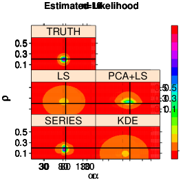
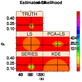
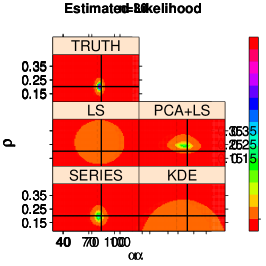
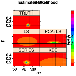
Figure 7: Comparison of level sets of estimated likelihood function ${\mathcal{L}}({\mathbf{x}};(\alpha,\rho))$ for the galaxy example for 4 samples sizes. Horizontal and vertical lines are the true values of the parameters. In all cases, the spectral series estimator gets closer to the real distribution, which is uncomputable in practice.

Spectral Series Density Ratio Estimator

Here we prove the bounds from the paper.

Define the following quantities:

$$\beta_{J}(\mathbf{x})=\sum_{j=1}^{J}\beta_{j}\psi_{j}(\mathbf{x}),\quad\beta_{j}=\int\psi_{j}(\mathbf{x})dF(\mathbf{x})$$

$$\widehat{\beta}_{J}(\mathbf{x})=\sum_{j=1}^{J}\widehat{\beta}_{i}\widehat{\psi}_{j}(\mathbf{x}),\quad\widehat{\beta}_{j}=\frac{1}{n_{F}}\sum_{k=1}^{n}\widehat{\psi}_{j}(\mathbf{x}^{F}_{k})$$

and note that

$$\int\left(\widehat{\beta}_{J}(\mathbf{x})-\beta(\mathbf{x})\right)^{2}dG(\mathbf{x}) \leq \int\left(\widehat{\beta}_{J}(\mathbf{x})-\beta_{J}(\mathbf{x})+\beta_{J}(\mathbf{x})-\beta(\mathbf{x})\right)^{2}dG(\mathbf{x})$$

$$\leq 2\left(\mbox{VAR}(\widehat{\beta}_{J}({\mathbf{x}}),\beta_{J}({\mathbf{x}}))+B(\beta_{J}({\mathbf{x}}),\beta({\mathbf{x}}))\right).$$

where

$$B(\beta({\mathbf{x}})_{J},\beta({\mathbf{x}}))\equiv\iint\left(\beta_{J}(\mathbf{x})-\beta(\mathbf{x})\right)^{2}dG(\mathbf{x})$$

can be interpreted as a bias term (or approximation error) and

$$\mbox{VAR}(\widehat{\beta}_{J}({\mathbf{x}}),\beta_{J}({\mathbf{x}}))\equiv\iint\left(\widehat{\beta}_{J}(\mathbf{x})-\beta_{J}(\mathbf{x})\right)^{2}dG(\mathbf{x})dz$$

can be interpreted as a variance term. First we bound the variance.

Lemma 1.

There exists $C>0$ such that $|\beta(\mathbf{x})|<C$ for all $\mathbf{x}\in\mathcal{X}$.

Proof.

Using Assumption 3 and the fact the kernel is bounded, it follows from the reproducing property and Cauchy-Schwartz inequality that

$$\beta(\mathbf{x})=\langle\beta(.),K(\mathbf{x},.)\rangle_{\mathcal{H}_{K_{\mathbf{x}}}}\leq||\beta(.)||_{\mathcal{H}_{K_{\mathbf{x}}}}\sqrt{K_{\mathbf{x}}(\mathbf{x},\mathbf{x})}<C$$

for some $C>0$. ∎

Lemma 2.

For all $1\leq j\leq J$,

$$\int\left(\widehat{\psi_{j}}(\mathbf{x})-\psi_{j}(\mathbf{x})\right)^{2}dG(\mathbf{x})=O_{P}\left(\frac{1}{\lambda_{j}\delta^{2}_{j}n_{G}}\right),$$

where $\delta_{j}=\lambda_{j}-\lambda_{j+1}$.

For a proof of Lemma 2 see, e.g., Sinha and Belkin (2009).

Lemma 3.

For all $1\leq j\leq J$,

$$\int\left(\widehat{\psi_{j}}(\mathbf{x})-\psi_{j}(\mathbf{x})\right)^{2}dF(\mathbf{x})=O_{P}\left(\frac{1}{\lambda_{j}\delta^{2}_{j}n_{G}}\right),$$

where $\delta_{j}=\lambda_{j}-\lambda_{j+1}$.

Proof.

It follows from Lemmas 1 and 2 that

$$\int\left(\widehat{\psi_{j}}(\mathbf{x})-\psi_{j}(\mathbf{x})\right)^{2}dF(\mathbf{x})=\int\left(\widehat{\psi_{j}}(\mathbf{x})-\psi_{j}(\mathbf{x})\right)^{2}\beta(\mathbf{x})dG(\mathbf{x})\leq$$

$$C\int\left(\widehat{\psi_{j}}(\mathbf{x})-\psi_{j}(\mathbf{x})\right)^{2}dG(\mathbf{x})=O_{P}\left(\frac{1}{\lambda_{j}\delta^{2}_{j}n_{G}}\right)$$

∎

Lemma 4.

For all $1\leq j\leq J$, there exists $C<\infty$ that does not depend on $n_{G}$ such that

$$E\left[\left(\widehat{\psi}_{j}(\mathbf{X}^{F})-\psi_{j}(\mathbf{X}^{F})\right)^{2}\right]<C.$$

Proof.

Let $\delta\in(0,1)$. From Sinha and Belkin (2009), it follows that

$${\mathbb{P}}\left(\int\left(\widehat{\psi}_{j}(\mathbf{x})-\psi_{j}(\mathbf{x})\right)^{2}dG(\mathbf{x})>\frac{16\log\left(\frac{2}{\delta}\right)}{\delta^{2}_{j}n_{G}}\right)<\delta,$$

and therefore for all $\epsilon>0$,

$${\mathbb{P}}\left(\int\left(\widehat{\psi}_{j}(\mathbf{x})-\psi_{j}(\mathbf{x})\right)^{2}dG(\mathbf{x})>\epsilon\right)<2e^{-\frac{\delta_{j}^{2}n_{G}\epsilon}{16}}.$$

Hence , using Lemma 1,

$${\mathbb{E}}\left[\left(\widehat{\psi}_{j}(\mathbf{X}^{F})-\psi_{j}(\mathbf{X}^{F})\right)^{2}\right]={\mathbb{E}}\left[\int\left(\widehat{\psi}_{j}(\mathbf{x})-\psi_{j}(\mathbf{x})\right)^{2}dF(\mathbf{x})\right]\leq C{\mathbb{E}}\left[\int\left(\widehat{\psi}_{j}(\mathbf{x})-\psi_{j}(\mathbf{x})\right)^{2}dG(\mathbf{x})\right]$$

$$\int_{0}^{\infty}{\mathbb{P}}\left(\int\left(\widehat{\psi}_{j}(\mathbf{x})-\psi_{j}(\mathbf{x})\right)^{2}dG(\mathbf{x})>\epsilon\right)d\epsilon\leq\int 2e^{-\frac{\delta_{j}^{2}n_{G}\epsilon}{16}}d\epsilon<\int 2e^{-\frac{\delta_{j}^{2}\epsilon}{16}}d\epsilon<\infty$$

∎

Lemma 5.

For all $1\leq j\leq J$, there exists $C<\infty$ that does not depend on $m$ such that

$${\mathbb{E}}\left[{\mathbb{V}}\left[\left(\widehat{\psi}_{j}(\mathbf{X}^{F})-\psi_{j}(\mathbf{X}^{F})\right)\bigg{|}\mathbf{X}^{G}_{1},\ldots,\mathbf{X}^{G}_{n_{G}}\right]\right]<C$$

Proof.

We have that

$${\mathbb{E}}\left[{\mathbb{V}}\left[\left(\widehat{\psi}_{j}(\mathbf{X}^{F})-\psi_{j}(\mathbf{X}^{F})\right)\bigg{|}\mathbf{X}^{G}_{1},\ldots,\mathbf{X}^{G}_{n_{G}}\right]\right]$$

$$\leq{\mathbb{V}}\left[\widehat{\psi}_{j}(\mathbf{X}^{F})-\psi_{j}(\mathbf{X}^{F})\right]\leq{\mathbb{E}}\left[\left(\widehat{\psi}_{j}(\mathbf{X}^{F})-\psi_{j}(\mathbf{X}^{F})\right)^{2}\right]$$

The result follows from Lemma 4. ∎

Lemma 6.

For all $1\leq j\leq J$,

$$\left[\frac{1}{n}\sum_{k=1}^{n}\left(\widehat{\psi}_{j}(\mathbf{X}^{F}_{k})-\psi_{j}(\mathbf{X}^{F}_{k})\right)-\int\left(\widehat{\psi}_{j}(\mathbf{x})-\psi_{j}(\mathbf{x})\right)dF(\mathbf{x})\right]^{2}=O_{P}\left(\frac{1}{n}\right)$$

Proof.

By Chebyshev’s inequality it holds that for all $M>0$

$${\mathbb{P}}\left(\left|\frac{1}{n}\sum_{k=1}^{n}\left(\widehat{\psi}_{j}(\mathbf{X}^{F}_{k})-\psi_{j}(\mathbf{X}^{F}_{k})\right)-\int\left(\widehat{\psi}_{j}(\mathbf{x})-\psi_{j}(\mathbf{x})\right)dF(\mathbf{x})\right|^{2}>M\bigg{|}\mathbf{X}^{G}_{1},\ldots,\mathbf{X}^{G}_{n_{G}}\right)\leq$$

$$\frac{1}{n_{F}M}{\mathbb{V}}\left[\left(\widehat{\psi}_{j}(\mathbf{X}^{F})-\psi_{j}(\mathbf{X}^{F})\right)\bigg{|}\mathbf{X}^{G}_{1},\ldots,\mathbf{X}^{G}_{n_{G}}\right].$$

The conclusion follows from taking an expectations with respect to sample from $G$ on both sides of the equation and using Lemma 5.

∎

Note that $\widehat{\psi}^{\prime}$s are random functions, and therefore the proof of Lemma 6 relies on the fact that these functions are estimated using a different sample than $\mathbf{X}_{1},\ldots,\mathbf{X}_{n}$.

Lemma 7.

For all $1\leq j\leq J$,

$$\left(\widehat{\beta}_{j}-\beta_{j}\right)^{2}=O_{P}\left(\frac{1}{n}\right)+O_{P}\left(\frac{1}{\lambda_{j}\delta^{2}_{j}n_{G}}\right).$$

Proof.

It holds that

$$\frac{1}{2}\left(\widehat{\beta}_{j}-\beta_{j}\right)^{2} \leq\left(\frac{1}{n_{F}}\sum_{k=1}^{n_{F}}\psi_{j}(\mathbf{X}^{F}_{k})-\beta_{j}\right)^{2}+\left(\frac{1}{n_{F}}\sum_{k=1}^{n_{F}}(\widehat{\psi}_{j}(\mathbf{X}^{F}_{k})-\psi_{j}(\mathbf{X}^{F}_{k}))\right)^{2}.$$

The first term is $O_{P}\left(\frac{1}{n_{F}}\right)$. The second term divided by two is bounded by

$$\frac{1}{2}\left(\frac{1}{n_{F}}\sum_{k=1}^{n_{F}}(\widehat{\psi}_{j}(\mathbf{X}^{F}_{k})-\psi_{j}(\mathbf{X}^{F}_{k}))-\int(\widehat{\psi}_{j}(\mathbf{x})-\psi_{j}(\mathbf{x}))dF(\mathbf{x})+\int(\widehat{\psi}_{j}(\mathbf{x})-\psi_{j}(\mathbf{x}))dF(\mathbf{x})\right)^{2}$$

$$\leq\left(\frac{1}{n_{F}}\sum_{k=1}^{n_{F}}(\widehat{\psi}_{j}(\mathbf{X}^{F}_{k})-\psi_{j}(\mathbf{X}^{F}_{k}))-\int(\widehat{\psi}_{j}(\mathbf{x})-\psi_{j}(\mathbf{x}))dF(\mathbf{x})\right)^{2}+\int(\widehat{\psi}_{j}(\mathbf{x})-\psi_{j}(\mathbf{x}))^{2}dF(\mathbf{x})$$

$$=O_{P}\left(\frac{1}{n_{F}}\right)+O_{P}\left(\frac{1}{\lambda_{j}\delta^{2}_{j}n_{G}}\right)$$

The result follows from Lemma 3.

∎

Lemma 8.

[Sinha and Belkin 2009, Corollary 1] Under the stated assumptions,

$$\int\widehat{\psi}_{j}^{2}(\mathbf{x})dG(\mathbf{x})=O_{P}\left(\frac{1}{\lambda_{j}\Delta^{2}_{J}n_{G}}\right)+1$$

and

$$\int\widehat{\psi}_{i}(\mathbf{x})\widehat{\psi}_{j}(\mathbf{x})dG(\mathbf{x})=O_{P}\left(\left(\frac{1}{\sqrt{\lambda_{i}}}+\frac{1}{\sqrt{\lambda_{j}}}\right)\frac{1}{\Delta_{J}\sqrt{n_{G}}}\right)$$

where $\Delta_{J}=\min_{1\leq j\leq J}\delta_{j}$.

Lemma 9.

Let $h(\mathbf{x})=\sum_{j=1}^{J}\beta_{j}\widehat{\psi}_{j}(\mathbf{x}).$ Then

$$\int\left|\widehat{\beta}_{J}(\mathbf{x})-h(\mathbf{x})\right|^{2}dG(\mathbf{x})=J\left(O_{P}\left(\frac{1}{n_{F}}\right)+O_{P}\left(\frac{1}{\lambda_{J}\Delta^{2}_{J}n_{G}}\right)\right).$$

Proof.

$$\int\left|\widehat{\beta}_{J}(z|\mathbf{x})-h(\mathbf{x})\right|^{2}dG(\mathbf{x})$$

$$=\sum_{j=1}^{J}\left(\widehat{\beta}_{j}-\beta_{j}\right)^{2}\int\widehat{\psi}_{j}^{2}(\mathbf{x})dG(\mathbf{x})+\sum_{j=1}^{J}\sum_{l=1,l\neq j}^{J}\left(\widehat{\beta}_{j}-\beta_{j}\right)\left(\widehat{\beta}_{l}-\beta_{l}\right)\int\widehat{\psi}_{j}(\mathbf{x})\widehat{\psi_{l}}(\mathbf{x})dG(\mathbf{x})$$

$$\sum_{j=1}^{J}\left(\widehat{\beta}_{j}-\beta_{j}\right)^{2}\int\widehat{\psi}_{j}^{2}(\mathbf{x})dG(\mathbf{x})+\left[\sum_{j=1}^{J}\left(\widehat{\beta}_{j}-\beta_{j}\right)^{2}\right]\left[\sqrt{\sum_{j=1}^{J}\sum_{l=1,l\neq j}^{J}\left(\int\widehat{\psi}_{j}(\mathbf{x})\widehat{\psi}_{l}(\mathbf{x})dG(\mathbf{x})\right)^{2}}\right]$$

where the last inequality follows from using Cauchy-Schwartz repeatedly. The result follows from Lemmas 7 and 8.

∎

Lemma 10.

Let $h(\mathbf{x})$ be as in Lemma 9. Then

$$\int\left|h(\mathbf{x})-\beta_{J}(\mathbf{x})\right|^{2}dG(\mathbf{x})=JO_{P}\left(\frac{1}{\lambda_{J}\Delta^{2}_{J}n_{G}}\right).$$

Proof.

Using Cauchy-Schwartz inequality,

$$\int\left|h(\mathbf{x})-\beta_{J}(\mathbf{x})\right|^{2}dG(\mathbf{x})\leq\int\left|\sum_{j=1}^{J}\beta_{j}\left(\psi_{j}(\mathbf{x)}-\widehat{\psi_{j}}(\mathbf{x})\right)\right|^{2}dG(\mathbf{x})$$

$$=\left\{\sum_{j=1}^{J}\beta^{2}_{j}\right\}\left\{\sum_{j=1}^{J}\int\left[\psi_{j}(\mathbf{x})-\widehat{\psi_{j}}(\mathbf{x})\right]^{2}dG(\mathbf{x})\right\}.$$

The conclusion follows from Lemma 2 and by noticing that $\sum_{j=1}^{J}\beta^{2}_{j}\leq||\beta(\mathbf{x})||^{2}<\infty$.

∎

It is now possible to bound the variance term:

Theorem 2.

Under the stated assumptions,

$$\mbox{VAR}(\widehat{\beta}_{J}({\mathbf{x}}),\beta_{J}({\mathbf{x}}))=J\left(O_{P}\left(\frac{1}{n_{F}}\right)+O_{P}\left(\frac{1}{\lambda_{J}\Delta^{2}_{J}n_{G}}\right)\right).$$

Proof.

Let $h$ be defined as in Lemma 9. We have

$$\frac{1}{2}\mbox{VAR}(\widehat{\beta}_{J}({\mathbf{x}}),\beta_{J}({\mathbf{x}}))=\frac{1}{2}\int\left|\widehat{\beta}_{J}(\mathbf{x})-h(\mathbf{x})+h(\mathbf{x})-\beta_{J}(\mathbf{x})\right|^{2}dG(\mathbf{x})$$

$$\leq\int\left|\widehat{\beta}_{J}(\mathbf{x})-h(\mathbf{x})\right|^{2}dG(\mathbf{x})+\int\left|h(\mathbf{x})-\beta_{J}(\mathbf{x})\right|^{2}dG(\mathbf{x}).$$

The conclusion follows from Lemmas 9 and 10.

∎

We now bound the bias term.

Lemma 11.

$\sum_{j\geq J}\beta_{j}^{2}=c_{K_{\mathbf{x}}}O(\lambda_{J})$.

Proof.

Note that $c_{K_{\mathbf{x}}}=||\beta(\mathbf{x})||^{2}_{\mathcal{H}}=\sum_{j\geq 1}\frac{\beta_{j}^{2}}{\lambda_{j}}$ (Minh, 2010). Using Assumption 3 and that the eigenvalues are decreasing it follows that

$$\sum_{j\geq J}\beta_{j}^{2}=\sum_{j\geq J}\beta_{j}^{2}\frac{\lambda_{j}}{\lambda_{j}}\leq\lambda_{J}||\beta(\mathbf{x})||^{2}_{\mathcal{H}},$$

and therefore $\sum_{j\geq J}\beta_{j}^{2}\leq\lambda_{J}c_{K_{\mathbf{x}}}=c_{K_{\mathbf{x}}}O(\lambda_{J})$.

∎

Theorem 3.

Under the stated assumptions, the bias is bounded by

$$B(\beta_{J}({\mathbf{x}}),\beta({\mathbf{x}}))=c_{K_{\mathbf{x}}}O(\lambda_{J}).$$

Proof.

By using orthogonality, we have that

$$B(\beta_{J}({\mathbf{x}}),\beta({\mathbf{x}})) \overset{\mbox{{def}}}{=}\int\left(\beta(\mathbf{x})-\beta_{J}(\mathbf{x})\right)^{2}dG(\mathbf{x})=\sum_{j>J}\beta^{2}_{j}.$$

The Theorem follows from Lemma 11. ∎

Spectral Series Likelihood Estimator

We now present similar bounds to those from shown for the Density Ratio estimator. To avoid confusions with the last section, from now on we denote by $\lambda^{\mathbf{x}}_{j}$ the eigenvalue $\lambda_{j}$ relative to the eigenfunction $\psi_{j}$, and by $\delta^{\mathbf{x}}_{j}$ its eigengap previously denoted by $\delta_{j}$.

In this section, we assume Assumption 1 and 2 from the last section, and, additionally:

Assumption 4.

For all $\mathbf{\theta}\in\Theta,$ let $g_{\theta}:\mathcal{X}\longrightarrow\Re;$ $g_{\theta}(\mathbf{x})={\mathcal{L}}(\mathbf{x};\theta)$. $g_{\theta}\in\mathcal{H}_{K_{\mathbf{x}}}(c_{\theta})\equiv\{g\in\mathcal{H}_{K_{\mathbf{x}}}:||g||^{2}_{\mathcal{H}_{K_{\mathbf{x}}}}\leq c_{\theta}^{2}\}$ where $c_{\theta}$’s are such that $c_{K_{\mathbf{x}}}\equiv\int_{\Theta}c_{\theta}^{2}dF(\theta)<\infty$.

Assumption 4 requires that for every $\theta\in\Theta$ fixed, ${\mathcal{L}}(\mathbf{x};\theta)$ is a smooth function of ${\mathbf{x}}$, where we again measure smoothness in a RKHS through its norm, and is analogous to Assumption 3. The last assumption we need is analogous to 4, and requires that for every ${\mathbf{x}}\in\mathcal{X}$ fixed, ${\mathcal{L}}(\mathbf{x};\theta)$ is a smooth function of $\theta$:

Assumption 5.

For all $\mathbf{x}\in\mathcal{X},$ let $h_{\mathbf{x}}:\Theta\longrightarrow\Re;$ $h_{\mathbf{x}}(\mathbf{\theta})={\mathcal{L}}(\mathbf{x};\theta)$. $h_{\mathbf{x}}\in\mathcal{H}_{K_{\theta}}(c_{\mathbf{x}})\equiv\{h\in\mathcal{H}_{K_{\theta}}:||h||^{2}_{\mathcal{H}_{K_{\theta}}}\leq c_{\mathbf{x}}^{2}\}$ where $c_{\mathbf{x}}$’s are such that $c_{K_{\theta}}\equiv\int_{\mathcal{X}}c_{\mathbf{x}}^{2}dG({\mathbf{x}})<\infty$.

First we note that an analogous decomposition of the loss

$$L\left(\widehat{{\mathcal{L}}},{\mathcal{L}}\right)=\int\left(\widehat{{\mathcal{L}}}(\mathbf{x};\theta)-{\mathcal{L}}(\mathbf{x};\theta)\right)^{2}dG(\mathbf{x})dF(\theta)$$

in terms of bias and variance holds. The proof that the bound on the variance term is analogous to the one of the variance bound of the density ratio estimator. The main difference is in Lemmas 2 and 8. We state and prove the new version of these in Lemmas 12 and 13. Notice that analogous Lemmas to 2 and 8 hold for basis $\phi_{i}$.

Lemma 12.

For all $1\leq i\leq I$ and for all $1\leq j\leq J$,

$$\iint\left(\widehat{\Psi_{i,j}}(\mathbf{\theta},\mathbf{x})-\Psi_{i,j}(\mathbf{\theta},\mathbf{x})\right)^{2}dG(\mathbf{x})dF(\mathbf{\theta})=O_{P}\left(\max\left\{\frac{1}{\lambda^{\mathbf{x}}_{j}\delta^{2}_{\mathbf{x},j}n_{G}},\frac{1}{\lambda^{\mathbf{\theta}}_{i}\delta^{2}_{\mathbf{\theta},i}n_{F}}\right\}\right)$$

,

Proof.

We have that

$$\frac{1}{2}\iint\left(\widehat{\Psi_{i,j}}(\mathbf{\theta},\mathbf{x})-\Psi_{i,j}(\mathbf{\theta},\mathbf{x})\right)^{2}dG(\mathbf{x})dF(\mathbf{\theta})\leq$$

$$\iint\left((\widehat{\phi}_{i}(\mathbf{\theta})-\phi_{i}(\mathbf{\theta}))\widehat{\psi}_{j}(\mathbf{x})+\phi_{i}(\mathbf{\theta})(\widehat{\psi}_{j}(\mathbf{x})-\psi_{j}(\mathbf{x}))\right)^{2}dG(\mathbf{x})dF(\mathbf{\theta})\leq$$

$$\int\widehat{\psi}_{j}^{2}(\mathbf{x})dG(\mathbf{x})\int(\widehat{\phi}_{i}(\mathbf{\theta})-\phi_{i}(\mathbf{\theta}))^{2}dF(\mathbf{\theta})+\int\phi^{2}_{i}(\mathbf{\theta})dF(\mathbf{\theta})\int(\widehat{\psi}_{j}(\mathbf{x})-\psi_{j}(\mathbf{x}))^{2}dG(\mathbf{x})$$

The results follows from orthonormality of $\phi_{i}$ wrt to $F(\mathbf{\theta})$, Lemmas 2 and 8. ∎

Lemma 13.

Under the stated assumptions, $\iint\widehat{\Psi}_{i,j}(\theta,\mathbf{x})\widehat{\Psi}_{k,l}(\theta,\mathbf{x})dG(\mathbf{x})dF(\theta)=$

$$=\left\{\begin{array}[]{l l}1+O_{P}\left(\max\left\{\frac{1}{\lambda^{\mathbf{x}}_{j}\delta^{2}_{\mathbf{x},j}n_{G}},\frac{1}{\lambda^{\mathbf{\theta}}_{i}\delta^{2}_{\mathbf{\theta},i}n_{F}}\right\}\right),&\text{if $i=k$ and $j=l$}\\ O_{P}\left(\left(\frac{1}{\sqrt{\lambda^{\mathbf{x}}_{l}}}+\frac{1}{\sqrt{\lambda^{\mathbf{x}}_{j}}}\right)\frac{1}{\Delta^{\mathbf{x}}_{J}\sqrt{n_{G}}}\right)&\text{if $i=k$ and $j\neq l$}\\ O_{P}\left(\left(\frac{1}{\sqrt{\lambda^{\theta}_{i}}}+\frac{1}{\sqrt{\lambda^{\theta}_{k}}}\right)\frac{1}{\Delta^{\theta}_{I}\sqrt{n_{F}}}\right)&\text{if $i\neq k$ and $j=l$}\\ O_{P}\left(\max\left\{\left(\frac{1}{\sqrt{\lambda^{\mathbf{x}}_{l}}}+\frac{1}{\sqrt{\lambda^{\mathbf{x}}_{j}}}\right)\frac{1}{\Delta^{\mathbf{x}}_{J}\sqrt{n_{G}}},\left(\frac{1}{\sqrt{\lambda^{\theta}_{i}}}+\frac{1}{\sqrt{\lambda^{\theta}_{k}}}\right)\frac{1}{\Delta^{\theta}_{I}\sqrt{n_{F}}}\right\}\right)&\text{if $i\neq k$ and $j\neq l$}\\ \end{array}\right.$$

Proof.

The proof of these facts follow from noticing that $\iint\widehat{\Psi}_{i,j}(\theta,\mathbf{x})\widehat{\Psi}_{k,l}(\theta,\mathbf{x})dG(\mathbf{x})dF(\theta)=\int\widehat{\psi}_{j}(\mathbf{x})\widehat{\psi}_{l}(\mathbf{x})dG(\mathbf{x})\int\phi_{i}(\theta)\phi_{k}(\theta)dF(\theta)$ and using Lemma 8 and its analogous for the basis $\phi_{i}$.

∎

The bound on the bias presents some additional differences to the proof of the bias bound from the ratio estimator, we therefore show it in details in the sequence.

Lemma 14.

For each $\theta\in\Theta,$ expand $g_{\theta}(\mathbf{x})$ into the basis $\psi:$ $g_{\theta}(\mathbf{x})=\sum_{j\geq 1}\alpha_{j}^{z}\psi_{j}(\mathbf{x}),$ where $\alpha_{j}^{\theta}=\int g_{\theta}(\mathbf{x})\psi_{j}(\mathbf{x})dG(\mathbf{x}).$ We have

$$\alpha_{j}^{\theta}=\sum_{i\geq 1}\beta_{i,j}\phi_{i}(\theta)\mbox{ and }\int\left(\alpha_{j}^{\theta}\right)^{2}dF(\theta)=\sum_{i\geq 1}\beta^{2}_{i,j}.$$

Proof.

It follows from projecting $\alpha_{j}^{\theta}$ into the basis $\phi$. ∎

Similarly, we have the following.

Lemma 15.

For each $\mathbf{x}\in\mathcal{X},$ expand $h_{\mathbf{x}}(\theta)$ into the basis $\phi:$ $h_{\mathbf{x}}(\theta)=\sum_{i\geq 1}\alpha_{i}^{\mathbf{x}}\phi_{i}(\theta),$ where $\alpha_{i}^{\mathbf{x}}=\int h_{\mathbf{x}}(\theta)\phi_{i}(\theta)dF(\theta).$ We have

$$\alpha_{i}^{\mathbf{x}}=\sum_{j\geq 1}\beta_{i,j}\psi_{i}(\mathbf{x})\mbox{ and }\int\left(\alpha_{i}^{\mathbf{x}}\right)^{2}dG(\mathbf{x})=\sum_{j\geq 1}\beta^{2}_{i,j}.$$

Lemma 16.

Using the same notation as Lemmas 14 and 15, we have

$$\beta_{i,j}=\int\alpha_{i}^{\mathbf{x}}\psi_{j}(\mathbf{x})dG(\mathbf{x})=\int\alpha_{j}^{\theta}\phi_{i}(\theta)dF(\theta).$$

Proof.

Follows from plugging the definitions of $\alpha_{i}^{\mathbf{x}}$ and $\alpha_{j}^{\theta}$ into the expressions above and recalling the definition of $\beta_{i,j}$. ∎

Lemma 17.

$\sum_{j\geq J}\int\left(\alpha_{j}^{\theta}\right)^{2}dF(\theta)=c_{K_{\mathbf{x}}}O(\lambda^{\mathbf{x}}_{J})$ and $\sum_{i\geq I}\int\left(\alpha_{i}^{\mathbf{x}}\right)^{2}dG({\mathbf{x}})=c_{K_{\theta}}O(\lambda^{\theta}_{I})$.

Proof.

Note that $||h_{\theta}(.)||^{2}_{\mathcal{H}_{K_{\mathbf{x}}}}=\sum_{j\geq 1}\frac{\left(\alpha^{\theta}_{j}\right)^{2}}{\lambda^{\mathbf{x}}_{j}}$ . Using Assumption 4 and that the eigenvalues are decreasing it follows that

$$\sum_{j\geq J}\left(\alpha^{\theta}_{j}\right)^{2}=\sum_{j\geq J}\left(\alpha^{\theta}_{j}\right)^{2}\frac{\lambda^{\mathbf{x}}_{j}}{\lambda^{\mathbf{x}}_{j}}\leq\lambda^{\mathbf{x}}_{J}||h_{\theta}(.)||^{2}_{\mathcal{H}_{K_{\mathbf{x}}}}\leq\lambda^{\mathbf{x}}_{J}c^{2}_{\theta},$$

and therefore $\sum_{j\geq J}\int\left(\alpha_{j}^{\theta}\right)^{2}dF(\theta)\leq\lambda^{\mathbf{x}}_{J}\int_{z}c_{\theta}^{2}dF(\theta)=c_{K_{\mathbf{x}}}O(\lambda^{\mathbf{x}}_{J})$. The proof of the second statement is analogous to this.

∎

Theorem 4.

Under the stated assumptions, the bias is bounded by

$$B({\mathcal{L}}_{I,J},{\mathcal{L}})=c_{K_{\mathbf{x}}}O\left(\lambda^{\mathbf{x}}_{J}\right)+c_{K_{\theta}}O(\lambda^{\theta}_{I}).$$

Proof.

By using orthogonality, we have that

$$B({\mathcal{L}}_{I,J},{\mathcal{L}}) \overset{\mbox{{def}}}{=}\iint\left({\mathcal{L}}(\mathbf{x};\theta)-{\mathcal{L}}_{I,J}(\mathbf{x},\theta)\right)^{2}dG(\mathbf{x})dF(\theta)\leq\sum_{j>J}\sum_{i\geq 1}\beta^{2}_{i,j}+\sum_{i>I}\sum_{j\geq 1}\beta^{2}_{i,j}$$

$$=\sum_{j\geq J}\int\left(\alpha_{j}^{\theta}\right)^{2}dF(\theta)+\sum_{i\geq I}\int\left(\alpha_{i}^{\mathbf{x}}\right)^{2}dG(\mathbf{x}),$$

where the last equality follows from Lemmas 14 and 15. The Theorem follows from Lemma 17 . ∎

References

• Aihara et al. (2011) H. Aihara et al. The eighth data release of the sloan digital sky survey: first data from SDSS-III. The Astrophysical Journal Supplement Series, 193(2):29, 2011.
• Beaumont (2010) M. A. Beaumont. Approximate bayesian computation in evolution and ecology. Annual Review of Ecology, Evolution, and Systematics, 41:379–406, 2010.
• Belabbas and Wolfe (2009) M. A. Belabbas and P. J Wolfe. Spectral methods in machine learning and new strategies for very large datasets. Proceedings of the National Academy of Sciences, 106(2):369–374, 2009.
• Bengio et al. (2004) Y. Bengio, O. Delalleau, N. Le Roux, J. F. Paiement, P. Vincent, and M. Ouimet. Learning eigenfunctions links Spectral Embedding and Kernel PCA. Neural Computation, 16(10):2197–2219, 2004.
• Bridle et al. (2009) S. Bridle et al. Handbook for the GREAT08 Challenge: An image analysis competition for cosmological lensing. The Annals of Applied Statistics, pages 6–37, 2009.
• Cameron and Pettitt (2012) E. Cameron and A.N. Pettitt. Approximate bayesian computation for astronomical model analysis: a case study in galaxy demographics and morphological transformation at high redshift. Monthly Notices of the Royal Astronomical Society, 425(1):44–65, 2012.
• Drineas and Mahoney (2005) P. Drineas and M.W. Mahoney. On the Nyström Method for approximating a Gram matrix for improved kernel-based learning. Journal of Machine Learning Research, 6, 2005.
• Efromovich (1999) S. Efromovich. Nonparametric Curve Estimation: Methods, Theory and Application. Springer, 1999.
• Estoup et al. (2012) A. Estoup, E. Lombaert, J. Marin, T. Guillemaud, P. Pudlo, C. P Robert, and J. Cornuet. Estimation of demo-genetic model probabilities with approximate bayesian computation using linear discriminant analysis on summary statistics. Molecular Ecology Resources, 12(5):846–855, 2012.
• Gretton et al. (2010) A. Gretton, A. Smola, J. Huang, M. Schmittfull, K. Borgwardt, and B. Schölkopf. Covariate shift by kernel mean matching. In J. Quionero-Candela, M. Sugiyama, A. Schwaighofer, and N. D. Lawrence, editors, Dataset Shift in Machine Learning, chapter 8. The MIT Press, 2010.
• Halko et al. (2011) N. Halko, P. G. Martinsson, and J. A. Tropp. Finding structure with randomness: Probabilistic algorithms for constructing approximate matrix decompositions. SIAM Review, 53(2):217–288, 2011.
• Hayfield and Racine (2008) T. Hayfield and J. S. Racine. Nonparametric econometrics: The np package. Journal of Statistical Software, 27(5), 2008.
• Hido et al. (2011) S. Hido, Y. Tsuboi, H. Kashima, M. Sugiyama, and T. Kanamori. Statistical outlier detection using direct density ratio estimation. Knowledge and Information Systems, 26(2):309–336, 2011.
• Ji et al. (2012) M. Ji, T. Yang, B. Lin, R. Jin, and J. Han. A simple algorithm for semi-supervised learning with improved generalization error bound. In ICML, 2012.
• Kanamori et al. (2009) T. Kanamori, S. Hido, and M. Sugiyama. A least-squares approach to direct importance estimation. Journal of Machine Learning Research, 10:1391–1445, 2009.
• Kanamori et al. (2012) T. Kanamori, T. Suzuki, and M. Sugiyama. Statistical analysis of kernel-based least-squares density-ratio estimation. Machine Learning, 86(3):335–367, 2012.
• Lee et al. (2010) A. B Lee, D. Luca, and K. Roeder. A spectral graph approach to discovering genetic ancestry. The Annals of Applied Statistics, 4(1):179, 2010.
• Lima et al. (2008) M. Lima, C.E. Cunha, H. Oyaizu, J. Frieman, H. Lin, and E. Sheldon. Estimating the redshift distribution of photometric galaxy samples. Monthly Notices of the Royal Astronomical Society, (390):118–130, 2008.
• Margolis (2011) A. Margolis. A literature review of domain adaptation with unlabeled data, March 2011. URL http://ssli.ee.washington.edu/~amargoli/review_Mar23.pdf.
• Marin et al. (2012) J. M. Marin, P. Pudlo, C. P Robert, and R. J Ryder. Approximate Bayesian computational methods. Statistics and Computing, 22(6):1167–1180, 2012.
• Minh (2010) H. Q. Minh. Some properties of Gaussian Reproducing Kernel Hilbert Spaces and their implications for function approximation and learning theory. Constructive Approximation, 32(2):307–338, 2010.
• Nam et al. (2012) H. H. Nam, H. Hachiya, and M. Sugiyama. Computationally efficient multi-label classification by least-squares probabilistic classifier. In Acoustics, Speech and Signal Processing (ICASSP), 2012 IEEE International Conference on, pages 2077–2080. IEEE, 2012.
• Rosasco et al. (2010) L. Rosasco, M. Belkin, and E. D. Vito. On learning with integral operators. The Journal of Machine Learning Research, 11:905–934, 2010.
• Sheldon et al. (2012) E. S. Sheldon, C. E. Cunha, R. Mandelbaum, J. Brinkmann, and B. A. Weaver. Photometric redshift probability distributions for galaxies in the SDSS DR8. The Astrophysical Journal Supplement Series, 201(2):32, 2012.
• Shimodaira (2000) H. Shimodaira. Improving predictive inference under covariate shift by weighting the log-likelihood function. Journal of Statistical Planning and Inference, 90(2):227–244, 2000.
• Sinha and Belkin (2009) K. Sinha and M. Belkin. Semi-supervised learning using sparse eigenfunction bases. In Y. Bengio, D. Schuurmans, J. Lafferty, C. K. I. Williams, and A. Culotta, editors, Advances in Neural Information Processing Systems 22, pages 1687–1695. 2009.
• Sugiyama et al. (2008) M. Sugiyama, T. Suzuki, S. Nakajima, H. Kashima, P. Bünau, and M. Kawanabe. Direct importance estimation for covariate shift adaptation. Annals of the Institute of Statistical Mathematics, 60(4):699–746, 2008.
• Sugiyama et al. (2010a) M. Sugiyama, T. Suzuki, and T. Kanamori. Density ratio estimation: A comprehensive review. RIMS Kokyuroku, pages 10–31, 2010a.
• Sugiyama et al. (2010b) M. Sugiyama, I. Takeuchi, T. Suzuki, T. Kanamori, H. Hachiya, and D. Okanohara. Conditional density estimation via least-squares density ratio estimation. In Proceedings of the Thirteenth International Conference on Artificial Intelligence and Statistics (AISTATS2010), pages 781–788, 2010b.
• Sugiyama et al. (2011) M. Sugiyama, M. Yamada, P. von Bünau, T. Suzuki, T. Kanamori, and M. Kawanabe. Direct density-ratio estimation with dimensionality reduction via least-squares hetero-distributional subspace search. Neural Networks, 24:183–198, 2011.
• Weyant et al. (2013) A. Weyant, C. Schafer, and W. M. Wood-Vasey. Likelihood-free cosmological inference with type ia supernovae: Approximate bayesian computation for a complete treatment of uncertainty. The Astrophysical Journal, 764(2):116, 2013.
• Zwald and Blanchard (2005) L. Zwald and G. Blanchard. On the convergence of eigenspaces in kernel principal component analysis. In NIPS, 2005.