The local standard of rest from data on young objects with account for the Galactic spiral density wave

Abstract

To estimate the peculiar velocity of the Sun with respect to the Local Standard of Rest (LSR), we used young objects in the Solar neighborhood with distance measurement errors within 10%–15%. These objects were the nearest Hipparcos stars of spectral classes O–B2.5, masers with trigonometric parallaxes measured by means of VLBI, and two samples of the youngest and middle-aged Cepheids. The most significant component of motion of all these stars is induced by the spiral density wave. As a result of using all these samples and taking into account the differential Galactic rotation, as well as the influence of the spiral density wave, we obtained the following components of the vector of the peculiar velocity of the Sun with respect to the LSR: $(U_{\odot},V_{\odot},W_{\odot})_{\mathrm{LSR}}=(6.0,10.6,6.5)\pm(0.5,0.8,0.3)\;\mathrm{km\,s}^{-1}$. We have found that components of the Solar velocity are quite insensitive to errors of the distance $R_{0}$ in a broad range of its values, from $R_{0}=7.5$ kpc to $R_{0}=8.5$ kpc, that affect the Galactic rotation curve parameters. In the same time, the Solar velocity components $(U_{\odot})_{\mathrm{LSR}}$ and $(V_{\odot})_{\mathrm{LSR}}$ are very sensitive to the Solar radial phase $\chi_{\odot}$ in the spiral density wave.

Introduction

The peculiar velocity of the Sun with respect to the LSR $(U_{\odot},V_{\odot},W_{\odot})_{\mathrm{LSR}}$ plays an important role in analysis of the kinematics of stars in the Galaxy. To properly analyze Galactic orbits, this motion should be removed from the observed velocities of stars, since it characterizes only the Solar orbit — namely, its deviation from the purely circular orbit. In particular, to build a Galactic orbit of the Sun, it is desirable to know the components $(U_{\odot},V_{\odot},W_{\odot})_{\mathrm{LSR}}$.

There are several ways to determine the peculiar velocity of the Sun with respect to the LSR. One of them is based on using the Str$\ddot{o}$mberg relation. The method consists in finding such values $(U_{\odot},V_{\odot},W_{\odot})_{\mathrm{LSR}}$ that correspond to zero stellar velocity dispersions (Dehnen & Binney, 1998; Bobylev & Bajkova, 2007; Aumer & Binney, 2009; Coçkunoğlu et al., 2011; Golubov et al., 2013). This method was addressed, for example, in the work by Schönrich et al. (2010), where the gradient of metallicity of stars in the Galactic disk was taken into account, and the velocity obtained is $(U_{\odot},V_{\odot},W_{\odot})_{\mathrm{LSR}}=(11.1,12.2,7.3)\pm(0.7,0.5,0.4)\;\mathrm{km\,s}^{-1}$.

Another method implies a search for such $(U_{\odot},V_{\odot},W_{\odot})_{\mathrm{LSR}}$ that lead to minimal stellar eccentricities. Using this approach, Francis & Anderson (2009) suggested that this velocity is $(U_{\odot},V_{\odot},W_{\odot})_{\mathrm{LSR}}=(7.5,13.5,6.8)\pm(1.0,0.3,0.1)\;\mathrm{km\,s}^{-1}$. To obtain this, 20000 local stars from the New Hipparcos Reduction (van Leeuwen, 2007) with known line-of-site velocities were used. Using the improved database of proper motions and line-of-site velocities of Hipparcos stars, XHIP, the same authors found the following new values: $(U_{\odot},V_{\odot},W_{\odot})_{\mathrm{LSR}}=(14.2,14.5,7.1)\pm(1.0,1.0,0.1)\;\mathrm{km\,s}^{-1}$ (Francis & Anderson, 2012); a great effort was made to get rid of the influence of inhomogeneous distribution of velocities of stars caused by kinematics of stellar groups and streams.

Another method is based on transferring stellar velocities towards their origin. Following this approach, Koval’ et al. (2009) derived the following values of $(U_{\odot},V_{\odot},W_{\odot})_{\mathrm{LSR}}=(5.1,7.9,7.7)\pm(0.4,0.5,0.2)\;\mathrm{km\,s}^{-1}.$

Experience in using the Str$\ddot{o}$mberg relation (Dehnen & Binney, 1998; Bobylev & Bajkova, 2007; Aumer & Binney, 2009) showed that the youngest stars significantly deviate from a linear dependence when analyzing $(V_{\odot})_{\mathrm{LSR}}$. This occurs when the dispersions $\sigma<17$ km s^-1(Dehnen & Binney, 1998). Therefore, the youngest stars are not normally used in this method. Cepheids and other youngest objects fall into this area, which allows us to include them in our analysis. This behavior of velocities of the youngest stars is primarily connected with the effect of the Galactic spiral density wave (Lin & Shu, 1964). For instance, the analysis of kinematics of 185 Galactic Cepheids by Bobylev & Bajkova (2012) demonstrated that perturbation velocities inferred by the spiral density wave can be determined with high confidence.

The purpose of this paper is to estimate the velocity $(U_{\odot},V_{\odot},W_{\odot})_{\mathrm{LSR}}$ using spatial velocities of the youngest objects in the Solar neighborhood that have parallax errors not larger than 10%–15%. For these stars, we consider not only the impact of the differential rotation of the Galaxy, but also the influence of the spiral density wave.

1 Method

Assuming that the angular rotation velocity of the Galaxy ($\Omega$) depends only on the distance $R$ from the axis of rotation, $\Omega=\Omega(R)$, the apparent velocity ${\bf V}(r)$ of a star at heliocentric radius ${\bf r}$ can be described in vectorial notation by the following relation (Eq. 2.86 in Ogorodnikov (1965))

$${\bf V}(r)=-{\bf V}_{\odot}+{\bf V_{\theta}}(R)-{\bf V_{\theta}}(R_{0})+{\bf V^{\prime}},$$ (1)

where ${\bf V}_{\odot}(U_{\odot},V_{\odot},W_{\odot})$ is the mean stellar sample velocity due to the peculiar Solar motion with respect to the LSR (hence its negative sign), the velocity $U$ is directed towards the Galactic center, $V$ is in the direction of Galactic rotation, $W$ is directed to the north Galactic pole; $R_{0}$ is the Galactocentric distance of the Sun; $R$ is the distance of an object from the Galactic rotation axis; ${\bf V_{\theta}}(R)$ is the circular velocity of the star with respect to the center of the Galaxy, ${\bf V_{\theta}}(R_{0})$ is the circular velocity of the Sun, while ${\bf V^{\prime}}$ are residual stellar velocities.

It is necessary to note that Eq. (1) is widely used by different authors for the Galaxy kinematics analysis (for example Eq. (6) in Mendez et al. (2000) or Eq. (4) in Vallenari et al. (2006)).

From the above relation (1), one can write down three equations in components ($V_{r},V_{l},V_{b}$), the so-called Bottlinger’s equations (Eq. 6.27 in Trumpler & Weaver (1953)):

$$\begin{array}[]{lllll}V_{r}=(\Omega-\Omega_{0})R_{0}\sin l\cos b,\\ V_{l}=(\Omega-\Omega_{0})R_{0}\cos l-\Omega r\cos b,\\ V_{b}=-(\Omega-\Omega_{0})R_{0}\sin l\sin b.\end{array}$$ (2)

These are exact formulas, and the signs of $\Omega$ follow Galactic rotation. The first of these equations was initially deduced by Bottlinger (1931), while the second one, even earlier, by Pilowski (1931), and the one for $V_{b},$ — by Ogorodnikov (1948). After expanding $\Omega$ into Taylor series against the small parameter $R-R_{0}$, then expanding the difference $R-R_{0}$, where the distance $R$ is

$$R^{2}=r^{2}\cos^{2}b-2R_{0}r\cos b\cos l+R^{2}_{0},$$ (3)

and then substituting the result into Eq. (2), one gets the equations of the Oort–Lindblad model (Eq. 6.34 in Trumpler & Weaver (1953)).

Our approach departs from the above in that the distances $r$ are known quite well. In this case, there is no need to expand $R-R_{0}$ into series, since the distance $R$ is calculated from Eq. (3).

Furthermore, our approach implies an extra assumption that the observed stellar velocities include perturbations due to the spiral density wave ${\bf V}_{sp}(V_{R},\Delta V_{\theta})$, with a linear dependence on both ${\bf V}_{sp}$ and ${\bf V}_{\odot}$. This allows us to write

$$-{\bf V}_{\odot}=-{{\bf V}_{\odot}}_{\mathrm{LSR}}+{\bf V}_{sp}.$$ (4)

Perturbations from the spiral density wave have a direct influence on the peculiar Solar velocity ${{\bf V}_{\odot}}_{\mathrm{LSR}}$, which appears to be first pointed out by Crézé & Mennessier (1973) — see the coefficients $a_{1}$ and $a_{2}$ in Eq. (22) of their paper. Then the relation (1) takes the following form:

$${\bf V}(r)=-{{\bf V}_{\odot}}_{\mathrm{LSR}}+{\bf V}_{sp}+{\bf V_{\theta}}(R)-{\bf V_{\theta}}(R_{0})+{\bf V^{\prime}},$$ (5)

which, considering the expansion of the angular velocity of Galactic rotation $\Omega$ into series up to the second order of $r/R_{0}$ reads

$$\begin{array}[]{lll}V_{r}=-U_{\odot}\cos b\cos l-V_{\odot}\cos b\sin l-W_{\odot}\sin b\\ +R_{0}(R-R_{0})\sin l\cos b\Omega^{\prime}_{0}\\ +0.5R_{0}(R-R_{0})^{2}\sin l\cos b\Omega^{\prime\prime}_{0}\\ +\Delta V_{\theta}\sin(l+\theta)\cos b-V_{R}\cos(l+\theta)\cos b,\end{array}$$ (6)

$$\begin{array}[]{lll}V_{l}=U_{\odot}\sin l-V_{\odot}\cos l\\ +(R-R_{0})(R_{0}\cos l-r\cos b)\Omega^{\prime}_{0}\\ +(R-R_{0})^{2}(R_{0}\cos l-r\cos b)0.5\Omega^{\prime\prime}_{0}-r\Omega_{0}\cos b\\ +\Delta V_{\theta}\cos(l+\theta)+V_{R}\sin(l+\theta),\end{array}$$ (7)

$$\begin{array}[]{lll}V_{b}=U_{\odot}\cos l\sin b+V_{\odot}\sin l\sin b-W_{\odot}\cos b\\ -R_{0}(R-R_{0})\sin l\sin b\Omega^{\prime}_{0}\\ -0.5R_{0}(R-R_{0})^{2}\sin l\sin b\Omega^{\prime\prime}_{0}\\ -\Delta V_{\theta}\sin(l+\theta)\sin b+V_{R}\cos(l+\theta)\sin b,\end{array}$$ (8)

where the following designations are used: $V_{r}$ is the line-of-sight velocity, $V_{l}=4.74r\mu_{l}\cos b$ and $V_{b}=4.74r\mu_{b}$ are the proper motion velocity components in the $l$ and $b$ directions, respectively, with the factor 4.74 being the quotient of the number of kilometers in an astronomical unit and the number of seconds in a tropical year; the star’s proper motion components $\mu_{l}\cos b$ and $\mu_{b}$ are in mas yr^-1, and the line-of-sight velocity $V_{r}$ is in km s^-1; $\Omega_{0}$ is the angular velocity of rotation at the distance $R_{0}$; parameters $\Omega^{\prime}_{0}$ and $\Omega^{\prime\prime}_{0}$ are the first and second derivatives of the angular velocity, respectively. To account for the influence of the spiral density wave, we used the simplest kinematic model based on the linear density wave theory by Lin & Shu (1964), where the potential perturbation is in the form of a travelling wave. Then,

$$V_{R}=f_{R}\cos\chi,$$ (9)

$$\Delta V_{\theta}=f_{\theta}\sin\chi,$$ (10)

where $f_{R}$ and $f_{\theta}$ are the amplitudes of the radial (directed toward the Galactic center in the arm) and azimuthal (directed along the Galactic rotation) velocity perturbations; $i$ is the spiral pitch angle ($i<0$ for winding spirals); $m$ is the number of arms (we take $m=2$ in this paper); $\theta$ is the star’s position angle measured in the direction of Galactic rotation: $\tan\theta=y/(R_{0}-x)$, where $x$ and $y$ are the Galactic heliocentric rectangular coordinates of the object; radial phase of the wave $\chi$ is

$$\chi=m[\cot(i)\ln(R/R_{0})-\theta]+\chi_{\odot},$$ (11)

where $\chi_{\odot}$ is the radial phase of the Sun in the spiral density wave; we measure this angle from the center of the Carina–Sagittarius spiral arm ($R\approx 7$ kpc). The parameter $\lambda$, which is the distance along the Galactocentric radial direction between adjacent segments of the spiral arms in the Solar neighborhood (the wavelength of the spiral density wave), is calculated from the relation $2\pi R_{0}/\lambda=m\cot(i).$

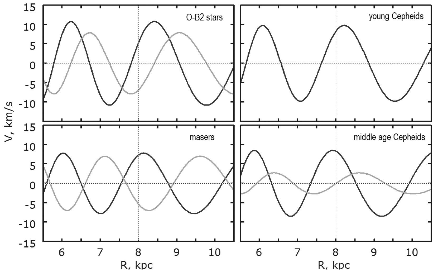
Figure 1: Radial ($V_{R}$, dark) and tangential ($\Delta V_{\theta}$, light) perturbation velocities versus Galactocentric distances $R$. Location of the Sun is indicated by a dotted line.

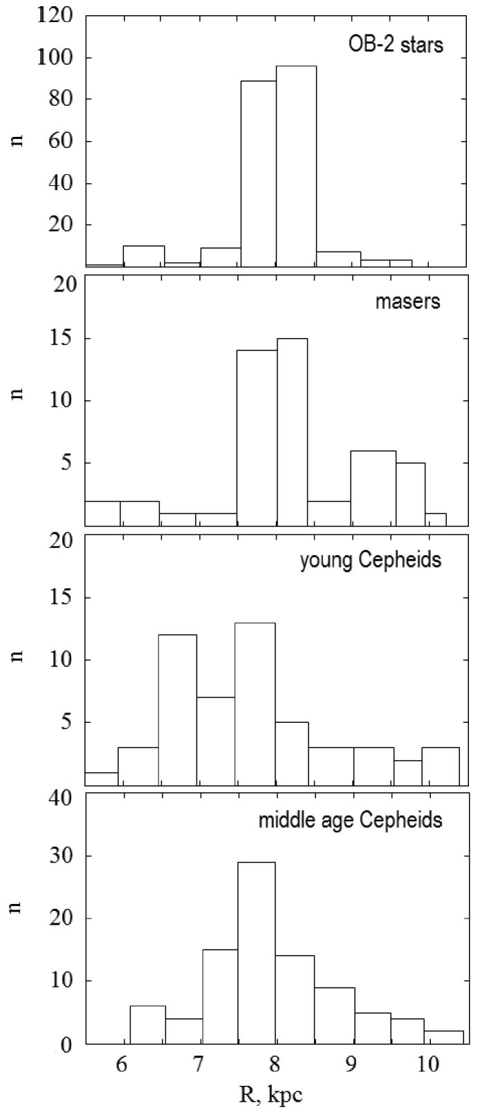
Figure 2: Number of stars versus Galactocentric distances $R$.

We take $R_{0}=8.0\pm 0.4$ kpc, according to analysis of the most recent determinations of this quantity in the review by Foster & Cooper (2010).

We use the well-known statistical method (Trumpler & Weaver, 1953; Ogorodnikov, 1965) to determine the parameters of the residual velocity (Schwarzschild) ellipsoid. It consists in determining the symmetric tensor of moments or the tensor of residual stellar velocity dispersions. When simultaneously using the stellar line-of-site velocities and proper motions to find the six unknown components of the dispersion tensor, we have six equations for each star. The semiaxes of the residual velocity ellipsoid, denoted by $\sigma_{1,2,3}$, can be determined by analyzing the eigenvalues of the dispersion tensor.

In the present paper, we assume that parameters of both the differential Galactic rotation and the spiral density wave are known from observations of distant stars and solving equations of the form (6)–(8). In this case the right-hand parts of the equations contain only components of the Solar peculiar velocity

$$\begin{array}[]{lll}V_{r}-R_{0}(R-R_{0})\sin l\cos b\Omega^{\prime}_{0}\\ -0.5R_{0}(R-R_{0})^{2}\sin l\cos b\Omega^{\prime\prime}_{0}\\ -\Delta V_{\theta}\sin(l+\theta)\cos b-V_{R}\cos(l+\theta)\cos b\\ =-U_{\odot}\cos b\cos l-V_{\odot}\cos b\sin l-W_{\odot}\sin b,\end{array}$$ (12)

$$\begin{array}[]{lll}V_{l}-(R-R_{0})(R_{0}\cos l-r\cos b)\Omega^{\prime}_{0}\\ -(R-R_{0})^{2}(R_{0}\cos l-r\cos b)0.5\Omega^{\prime\prime}_{0}+r\Omega_{0}\cos b\\ -\Delta V_{\theta}\cos(l+\theta)-V_{R}\sin(l+\theta)\\ =U_{\odot}\sin l-V_{\odot}\cos l,\end{array}$$ (13)

$$\begin{array}[]{lll}V_{b}+R_{0}(R-R_{0})\sin l\sin b\Omega^{\prime}_{0}\\ +0.5R_{0}(R-R_{0})^{2}\sin l\sin b\Omega^{\prime\prime}_{0}\\ +\Delta V_{\theta}\sin(l+\theta)\sin b+V_{R}\cos(l+\theta)\sin b\\ =U_{\odot}\cos l\sin b+V_{\odot}\sin l\sin b-W_{\odot}\cos b.\\ \end{array}$$ (14)

The system (12)–(LABEL:EQ-103) can be solved by least-squares adjustment with respect to three unknowns $U_{\odot},$ $V_{\odot}$, and $W_{\odot}$. Another approach (which we follow) is to calculate components of spatial velocities $U,V,W$ of stars:

$$\begin{array}[]{lll}U=V^{\prime}_{r}\cos l\cos b-V^{\prime}_{l}\sin l-V^{\prime}_{b}\cos l\sin b,\\ V=V^{\prime}_{r}\sin l\cos b+V^{\prime}_{l}\cos l-V^{\prime}_{b}\sin l\sin b,\\ W=V^{\prime}_{r}\sin b+V^{\prime}_{b}\cos b,\end{array}$$ (15)

where $V^{\prime}_{r},V^{\prime}_{l},V^{\prime}_{b}$ are left-hand parts of Eqs. (12)–(LABEL:EQ-103) which are the observed stellar velocities free from Galactic rotation and the spiral density wave. Then ${\overline{U}=-U_{\odot}},$ ${\overline{V}=-V_{\odot}}$ and ${\overline{W}=-W_{\odot}}$.

2 Data

2.1 O–B2.5 stars

The sample of selected 200 massive ($<$10$M_{\odot}$) stars of spectral classes O–B2.5 is described in detail in our previous paper (Bobylev & Bajkova, 2013a). It contains spectral binary O stars with reliable kinematic characteristics from the $3$ kpc Solar neighborhood. In addition, the sample contains 124 Hipparcos (van Leeuwen, 2007) stars of spectral types from B0 to B2.5 whose parallaxes were determined to within 10% and better and for which there are line-of-sight velocities in the catalog by Gontcharov (2006).

In this work we solve the problem of determining the peculiar velocity of the Sun. This problem can be solved most reliable using the closest stars to the Sun. Therefore, from the database, including 200 stars, we have selected 161 stars from the Solar neighborhood of $0.7$ kpc radius.

Parameters of the Galactic rotation and the spiral density wave used for reduction of motion of these stars were determined in (Bobylev & Bajkova, 2013a) using full sample of 200 stars, because for determination of Galactic parameters it is important to have distant stars as well: $\Omega_{0}=32.4\pm 1.1$ km s^-1 kpc${}^{-1},$ $\Omega^{\prime}_{0}=-4.33\pm 0.19$ km s^-1 kpc${}^{-2},$ $\Omega^{\prime\prime}_{0}=0.77\pm 0.42$ km s^-1 kpc${}^{-3},$ $f_{R}=-10.8\pm 1.2$ km s${}^{-1},$ $f_{\theta}=7.9\pm 1.3$ km s${}^{-1},$ $\chi_{\odot}=-120^{\circ}\pm 4^{\circ}.$ For all samples in the present work, we use the same value of the wavelength $\lambda=2.6\pm 0.2$ kpc ($i=-6.0\pm 0.4^{\circ}$ for $m=2$).

2.2 Masers

We use coordinates and trigonometric parallaxes of masers measured by VLBI with errors of less than 10% in average. These masers are connected with very young objects (basically proto stars of high masses, but there are ones with low masses too; a number of massive super giants are known as well) located in active star-forming regions.

One of such observational campaigns is the Japanese project VERA (VLBI Exploration of Radio Astrometry) for observations of water (H₂O) Galactic masers at 22 GHz (Hirota et al., 2007) and SiO masers (which occur very rarely among young objects) at 43 GHz (Kim et al., 2008). Water and methanol (CH₃OH) maser parallaxes are observed in USA (VLBA) at 22 GHz and 12 GHz (Reid et al., 2009). Methanol masers are observed also in the framework of the European VLBI network (Rygl et al., 2010). Both these projects are joined together in the BeSSeL program (Brunthaler et al., 2011). VLBI observations of radio stars in continuum at 8.4 GHz (Dzib et al., 2011) are carried out with the same goals.

In the present work, we use only data on the nearby maser sources, which are located no farther than 1.5 kpc from the Sun. All required information about 30 such masers is given in the work by Xu et al. (2013), which is dedicated to the study of the Local arm (the Orion arm).

By applying the reduction algorithm, we use the following parameters of the Galactic rotation and the spiral density wave found by Bobylev & Bajkova (2013b): $\Omega_{0}=29.9\pm 1.1$ km s^-1 kpc${}^{-1},$ $\Omega^{\prime}_{0}=-4.27\pm 0.20$ km s^-1 kpc${}^{-2},$ $\Omega^{\prime\prime}_{0}=0.915\pm 0.166$ km s^-1 kpc${}^{-3},$ $f_{R}=-7.8\pm 0.7$ km s${}^{-1},$ $f_{\theta}=7.0\pm 1.2$ km s^-1. In this case, the values of the phase of the Sun in the spiral wave found independently from radial and tangential perturbations using Fourier analysis are different: $(\chi_{\odot})_{R}=-160^{\circ}\pm 15^{\circ}$ and $(\chi_{\odot})_{\theta}=-50^{\circ}\pm 15^{\circ}$, respectively.

Note that line-of-site velocities of masers given in the literature usually refer to the standard apex of the Sun. So we fix such line-of-site velocities, making them heliocentric.

Table 1: Components of the peculiar velocity of the Sun with respect to the LSR, calculated considering the differential Galactic rotation only.

Stars	$U_{\odot}$	$V_{\odot}$	$W_{\odot}$	$N_{\star}$	distance	$\sigma_{1}$	$\sigma_{2}$	$\sigma_{3}$
	km s-1	km s-1	km s-1		kpc	km s-1	km s-1	km s-1
O–B2.5	$10.0\pm 1.0$	$14.7\pm 1.3$	$7.2\pm 0.7$	161	$<0.7$	$7.3\pm 0.5$	$5.7\pm 0.6$	$3.9\pm 0.4$
masers	$11.9\pm 2.7$	$16.2\pm 3.4$	$6.2\pm 1.7$	26	$<1.5$	$6.0\pm 0.7$	$5.7\pm 0.6$	$3.0\pm 1.7$
Cepheids, $P\geq 9^{\mathrm{d}}$	$6.5\pm 2.3$	$12.0\pm 2.4$	$6.1\pm 2.5$	36	$<2$	$12.2\pm 1.3$	$10.5\pm 0.8$	$5.9\pm 4.8$
Cepheids, $5^{\mathrm{d}}\leq P<9^{\mathrm{d}}$	$7.3\pm 2.1$	$11.1\pm 2.0$	$6.4\pm 1.8$	74	$<2$	$14.4\pm 2.2$	$10.3\pm 2.0$	$9.5\pm 3.6$

Table 2: Components of the vector of the peculiar velocity of the Sun with respect to the LSR, calculated considering both the differential Galactic rotation and the spiral density wave.

Stars	$U_{\odot}$	$V_{\odot}$	$W_{\odot}$	$N_{\star}$	distance	$\sigma_{1}$	$\sigma_{2}$	$\sigma_{3}$
	km s-1	km s-1	km s-1		kpc	km s-1	km s-1	km s-1
O–B2.5	$4.6\pm 0.7$	$8.6\pm 0.9$	$7.2\pm 0.7$	161	$<0.7$	$6.0\pm 0.5$	$5.8\pm 0.5$	$3.7\pm 0.4$
masers	$6.0\pm 1.6$	$11.4\pm 2.5$	$6.2\pm 1.7$	26	$<1.5$	$6.2\pm 0.4$	$4.8\pm 0.6$	$3.6\pm 1.5$
Cepheids, $P\geq 9^{\mathrm{d}}$	$6.8\pm 2.3$	$12.1\pm 2.4$	$6.1\pm 2.5$	36	$<2$	$11.4\pm 1.3$	$10.0\pm 0.9$	$5.6\pm 5.1$
Cepheids, $5^{\mathrm{d}}\leq P<9^{\mathrm{d}}$	$6.7\pm 2.1$	$10.4\pm 1.9$	$6.4\pm 1.8$	74	$<2$	$14.7\pm 2.3$	$9.8\pm 1.9$	$9.3\pm 3.7$
average	$6.0\pm 0.5$	$10.6\pm 0.8$	$6.5\pm 0.3$

2.3 Cepheids

We used the data on classical Cepheids with proper motions mainly from the Hipparcos catalog and line-of-sight velocities from the various sources. The data from Mishurov et al. (1997) and Gontcharov (2006), as well as from the SIMBAD database, served as the main sources of line-of-sight velocities for the Cepheids. For several long-period Cepheids, we used their proper motions from the TRC (Høg et al., 1998) and UCAC4 (Zacharias et al., 2013) catalogs.

To calculate the Cepheid distances, we use the calibration from Fouqu et al. (2007),

$$\langle M_{V}\rangle=-1.275-2.678\log P,$$ (16)

where the period $P$ is in days. Given $\langle M_{V}\rangle$, taking the period-averaged apparent magnitudes $\langle V\rangle$ and extinction $A_{V}=3.23E(\langle B\rangle-\langle V\rangle)$ mainly from Acharova et al. (2012) and, for several stars, from Feast & Whitelock (1997), we determine the distance $r$ from the relation

$$r=10^{\displaystyle-0.2(\langle M_{V}\rangle-\langle V\rangle-5+A_{V})}$$ (17)

and then assume that the relative error of Cepheid distances determined by this method is 10%.

We divided the entire sample into two parts, depending on the pulsation period, which well reflects the mean Cepheid age ($t$). We use the calibration from Efremov (2003),

$$\log t=8.50-0.65\log P,$$ (18)

obtained by analyzing Cepheids in the Large Magellanic Cloud.

Parameters of the Galactic rotation and spiral density wave depend on the age of the Cepheids. Therefore, for each sample of Cepheids of the given age, these effects should be addressed individually. We use the values of the parameters found in the work by Bobylev & Bajkova (2012) for three age groups. The youngest Cepheids with periods of $P\geq 9^{\mathrm{d}}$ are characterized by the average age of $55$ Myr, middle-aged Cepheids with periods of $5^{\mathrm{d}}\leq P<9^{\mathrm{d}}$ have the average age of $95$ Myr, while the oldest Cepheids with periods of $P<5^{\mathrm{d}}$ have that of $135$ Myr. In the present work, a sample of old Cepheids is not used because there are very few of them in the Solar neighborhood, and their kinematic parameters are not very reliable.

According to Bobylev & Bajkova (2012), for the youngest Cepheids with periods of $P\geq 9^{\mathrm{d}}$ $\Omega_{0}=26.1\pm 0.9$ km s^-1 kpc^-1, $\Omega^{\prime}_{0}=-3.95\pm 0.13$ km s^-1 kpc^-2, $\Omega^{\prime\prime}_{0}=0.79\pm 0.10$ km s^-1 kpc^-3, $f_{R}=-9.8\pm 1.3$ km s^-1, $\chi_{\odot}=-148^{\circ}\pm 14^{\circ}$, and the value of velocity perturbations in the tangential direction $f_{\theta}$ is assumed to be zero.

For middle-aged Cepheids with $(5^{\mathrm{d}}\leq P<9^{\mathrm{d}})$ $\Omega_{0}=30.4\pm 1.0$ km s^-1 kpc^-1, $\Omega^{\prime}_{0}=-4.34\pm 0.13$ km s^-1 kpc^-2, $\Omega^{\prime\prime}_{0}=0.69\pm 0.14$ km s^-1 kpc^-3, $f_{R}=-8.5\pm 1.1$ km s^-1, $f_{\theta}=2.7\pm 1.1$ km s^-1. The values for the phase of the Sun in the spiral wave found separately from radial and tangential perturbations by periodogram analysis based on Fourier transform slightly differ: $(\chi_{\odot})_{R}=-193^{\circ}\pm 9^{\circ}$ and $(\chi_{\odot})_{\theta}=-180^{\circ}\pm 9^{\circ}.$

In Fig. 2, we show the histograms of stellar distribution in the samples under analysis versus Galactocentric distances $R$. To make these plots, we took stars in the $r<2.5$ kpc vicinity. One can see that the distributions of OB-2.5 stars and masers are similar. This is due to the fact that nearby masers belong to the Local arm, while the OB-2.5 star sample is essentially the Gould belt (since we chose the stars with $\sigma_{\pi}/\pi<10\%$) that is a part of the Local arm. Cepheids of different ages manifest the well-known effect – a gradient of the age across the spiral arm (Pavlovskaya & Suchkov, 1978), which suggests that the spiral arm goes towards the Galactic center.

3 Results and Discussion

3.1 The fixed value of $R_{0}$

Here we describe the results obtained at fixed value of $R_{0}=8$ kpc, assuming the parameters of differential Galactic rotation and the spiral density wave calculated earlier independently for each stellar sample.

In Figure 1, there are radial ($V_{R}$) and tangential ($\Delta V_{\theta}$) velocities of perturbations vs Galactocentric distance $R$, induced by the spiral density wave. These velocities are calculated according to the formulas (9), (10), and (11) assuming $\theta=0^{\circ}$, and the amplitudes of perturbations $f_{R}$ and $f_{\theta}$ defined in the data description (Section 2). As it can be seen from this figure, at $R=R_{0}$, the perturbations achieve about $5$ km s^-1 in the radial direction. In the tangential direction, the same value is achieved for two samples: of youngest O–B2 stars and of masers. In the case of young Cepheids, perturbations in the tangential direction are not significant. In the case of middle-aged Cepheids, perturbations in the tangential direction at $R=R_{0}$ are close to zero. Note that a very small Solar neighborhood ($R\rightarrow R_{0}$) is crucial to determine the velocity $(U_{\odot},V_{\odot},W_{\odot})_{\mathrm{LSR}}$.

In Table 1, the components of the peculiar velocity of the Sun with respect to the LSR $(U_{\odot},V_{\odot},W_{\odot})_{\mathrm{LSR}}$ are given. They were obtained only taking into account the influence of the differential Galactic rotation. Components of this vector, given in Table 2, were calculated considering both the effects of the differential Galactic rotation and of the spiral density wave. In the last three columns of Tables 1–2, the main axes of the ellipsoid of residual velocities $\sigma_{1},\sigma_{2},\sigma_{3}$ are given. We should note that, after considering the perturbations from the spiral density wave, the values of residual velocity dispersions $\sigma_{1},\sigma_{2},\sigma_{3}$ have slightly different distributions, which leads to a changed orientation of the residual velocity ellipsoid. However, a detailed analysis of this problem is out of the scope of the present study and will be conducted elsewhere.

As it is seen from Tables 1 and 2, considering the effect of the spiral density wave for O–B2.5 stars and for masers leads to a considerable variation of the components $\Delta U_{\odot}$ and $\Delta V_{\odot}$ by $\approx$6 km^-1. In addition, this gives smaller errors of the velocity $(U_{\odot},V_{\odot},W_{\odot})_{\mathrm{LSR}}$, which is especially noticeable for masers.

The velocity $(V_{\odot})_{\mathrm{LSR}}$ (Table 1) found from the data on masers differs from $(V_{\odot})_{\mathrm{LSR}}=12.2\;\mathrm{km\,s}^{-1}$(Schönrich et al., 2010) by $\approx$4 km s^-1, which is in accordance with the result of analysis of masers in the Local arm (Xu et al., 2013).

The following average values of the parameters $(U_{\odot},V_{\odot},W_{\odot})_{\mathrm{LSR}}$ found in the present work are, essentially, more accurate than the estimate $(U_{\odot},V_{\odot},W_{\odot})_{\mathrm{LSR}}=(5.5,11.0,8.5)\pm(2.2,1.7,1.2)\;\mathrm{km\,s}^{-1}$ obtained from 28 masers by Bobylev & Bajkova (2010) considering the influence of the spiral density wave. The average value of $(V_{\odot})_{\mathrm{LSR}}$ (Table 2) is in a good agreement with the result by Schönrich et al. (2010). There is a discrepancy in the $(U_{\odot})_{\mathrm{LSR}}$ component with Schönrich et al. (2010), and especially with Francis & Anderson (2012).

Note that the revised Str$\ddot{o}$mberg relation applied to the experimental RAVE data gives an absolutely different velocity $(V_{\odot})_{\mathrm{LSR}}\approx 3\;\mathrm{km\,s}^{-1}$ (Golubov et al., 2013). Using another approach to analysis of RAVE data Pasetto et al. (2012) obtained the following velocities: $(U_{\odot},V_{\odot})_{\mathrm{LSR}}=(9.87,8.01)\pm(0.37,0.29)\;\mathrm{km\,s}^{-1}$.

Thus different methods give different results, and a final agreement on the values of the velocity $(U_{\odot},V_{\odot},W_{\odot})_{\mathrm{LSR}}$ is not achieved till now. We consider our estimates most reliable as they are based on the youngest stars characterized by a small velocity dispersion and by small Galactic orbit eccentricities as well.

In Fig. 3, there is a histogram of Galactic orbital eccentricities for the OB-2.5 star sample. One can see that eccentricities of the stars considered are indeed small. Note that we have excluded escaping stars when making this sample (Bobylev & Bajkova, 2013a).

Figure 3: Number of stars versus eccentricity $e$.

Table 3: Components of the vector of the peculiar velocity of the Sun with respect to the LSR, calculated considering both the differential Galactic rotation and the spiral density wave for three values of $R_{0}=7.5,8.0,8.5$ kpc.

$R_{0}$		$7.5$ kpc				$8.0$ kpc				$8.5$ kpc
Stars	$U_{\odot}$	$V_{\odot}$	$W_{\odot}$		$U_{\odot}$	$V_{\odot}$	$W_{\odot}$		$U_{\odot}$	$V_{\odot}$	$W_{\odot}$
	km s-1	km s-1	km s-1		km s-1	km s-1	km s-1		km s-1	km s-1	km s-1
O–B2.5	$4.9\pm 0.5$	$8.6\pm 0.5$	$7.2\pm 0.3$		$4.8\pm 0.5$	$8.6\pm 0.5$	$7.2\pm 0.3$		$4.8\pm 0.5$	$8.5\pm 0.5$	$7.2\pm 0.3$
masers	$5.5\pm 1.5$	$11.3\pm 2.5$	$6.2\pm 1.7$		$6.0\pm 1.6$	$11.4\pm 2.5$	$6.2\pm 1.7$		$5.4\pm 1.5$	$11.5\pm 2.5$	$6.2\pm 1.7$
Ceph., $P\geq 9^{\mathrm{d}}$	$6.1\pm 2.3$	$10.5\pm 2.2$	$6.1\pm 2.5$		$6.6\pm 2.5$	$10.6\pm 2.2$	$6.1\pm 2.5$		$7.0\pm 2.6$	$10.7\pm 2.2$	$6.1\pm 2.5$
$5^{\mathrm{d}}\leq P<9^{\mathrm{d}}$	$7.0\pm 2.1$	$10.8\pm 1.9$	$6.4\pm 1.8$		$6.7\pm 2.1$	$10.8\pm 2.0$	$6.4\pm 1.8$		$6.5\pm 2.1$	$10.9\pm 2.0$	$6.4\pm 1.8$

Table 4: Components of the vector of the peculiar velocity of the Sun with respect to the LSR, calculated considering both the differential Galactic rotation and the spiral density wave for the different values of $\chi_{\odot}.$

$\chi_{\odot}$	$-80^{\circ}$		$-110^{\circ}$		$-120^{\circ}$		$-130^{\circ}$		$-160^{\circ}$
	$U_{\odot}$	$V_{\odot}$	$U_{\odot}$	$V_{\odot}$	$U_{\odot}$	$V_{\odot}$	$U_{\odot}$	$V_{\odot}$	$U_{\odot}$	$V_{\odot}$
	km s-1	km s-1	km s-1	km s-1	km s-1	km s-1	km s-1	km s-1	km s-1	km s-1
O–B2.5	$11.4\pm 0.5$	$7.6\pm 0.6$	$6.3\pm 0.5$	$8.0\pm 0.6$	$4.8\pm 0.5$	$8.6\pm 0.5$	$3.5\pm 0.5$	$9.3\pm 0.3$	$0.8\pm 0.6$	$12.5\pm 0.5$

3.2 Errors of Galactic Rotation Parameters

Here we describe the results obtained for three particular values of $R_{0}=7.5,8.0,8.5$ kpc using the corresponding differential Galactic rotation parameters. That is, we now use one and the same Galactic rotation curve to analyze each of the stellar samples. Amplitudes of perturbation velocities of the spiral density wave $f_{R}$ and $f_{\theta}$, as well as the values of the Solar phase $\chi_{\odot}$ in the spiral wave, are chosen as above in Section 3.1.

For this purpose, we took a sample of masers (55 masers, $\sigma_{\pi}/\pi<10\%,$ $r<3.5$ kpc) from Bobylev & Bajkova (2013b) and, taking three fixed values of $R_{0}$, found the following parameters of the Galactic rotation curve:

$$\begin{array}[]{lll}R_{0}=7.5~{}\hbox{kpc,}\\ \Omega_{0}=30.0\pm 1.1~{}\hbox{km s${}^{-1}$ kpc${}^{-1},$}\\ \Omega^{\prime}_{0}=-4.61\pm 0.21~{}\hbox{km s${}^{-1}$ kpc${}^{-2},$}\\ \Omega^{\prime\prime}_{0}=1.081\pm 0.180~{}\hbox{km s${}^{-1}$ kpc${}^{-3},$}\end{array}$$ (19)

$$\begin{array}[]{lll}R_{0}=8.0~{}\hbox{kpc,}\\ \Omega_{0}=29.9\pm 1.1~{}\hbox{km s${}^{-1}$ kpc${}^{-1},$}\\ \Omega^{\prime}_{0}=-4.27\pm 0.20~{}\hbox{km s${}^{-1}$ kpc${}^{-2},$}\\ \Omega^{\prime\prime}_{0}=0.915\pm 0.166~{}\hbox{km s${}^{-1}$ kpc${}^{-3},$}\end{array}$$ (20)

$$\begin{array}[]{lll}R_{0}=8.5~{}\hbox{kpc,}\\ \Omega_{0}=29.8\pm 1.1~{}\hbox{km s${}^{-1}$ kpc${}^{-1},$}\\ \Omega^{\prime}_{0}=-3.98\pm 0.18~{}\hbox{km s${}^{-1}$ kpc${}^{-2},$}\\ \Omega^{\prime\prime}_{0}=0.783\pm 0.154~{}\hbox{km s${}^{-1}$ kpc${}^{-3}.$}\end{array}$$ (21)

Parameters (20) are the same as those used previously for the maser sample in Section 3.1.

The results are summarized in Table 3, where one can see that there is no considerable departure from the previous results (Table 2). The only noticeable difference is for the sample of young Cepheids, $\Delta V_{\odot}\approx 2$ km s^-1, which is due to the difference in Galactic rotation rate $\Delta\Omega_{0}\approx 2$ km s^-1. As early as in the paper of Feast & Whitelock (1997) it was already noted that the youngest Cepheids, for some unknown reason, rotate slightly slower than the older ones. In this sense, we consider the approach taken in the previous paragraph as more adequate to the goal of the present study: it is better to apply individual rotation curves to each stellar sample.

3.3 Errors of the Spiral Wave Parameters

Here we describe our results for several model values of the Solar phase $\chi_{\odot}$ in the spiral density wave for a sample of O–B2.5 stars (161 stars, $r<0.7$ kpc). We used the Galactic rotation curve parameters (20).

The results are reflected in Table 4 whence one can see that the Solar velocity components $U_{\odot}$ and $V_{\odot}$ are very sensitive to the above parameter ($W_{\odot}$ velocities are not shown in the Table as they are practically not affected by the density wave).

It is easy to understand these results by analyzing the corresponding panel of Fig. 1 and Table 1. For instance, for $\chi_{\odot}=-160^{\circ}$, the radial perturbation curve ($V_{R}$) is near its maximum, so the influence to the $U_{\odot}$ component is most prominent. On the contrary, the tangential perturbation curve ($\Delta V_{\theta}$) is about zero, so there is no effect on the $V_{\odot}$ component.

We must note that, in our previous paper (Bobylev & Bajkova, 2013a), the uncertainty of $R_{0}$ was not taken into account when determining the Solar phase in the spiral density wave $\chi_{\odot}=-120\pm 4^{\circ}$. We have redone Monte Carlo simulation and obtained the following results:

1. If we consider only the error $\sigma_{R_{0}}=0.4$ kpc, its effect on the uncertainty of the Solar phase in the spiral density wave becomes very small: $\sigma_{\chi_{\odot}}=0.2^{\circ}$. The explanation for this is that when you change $R_{0},$ the length of a wave stretches like a rubber band, but the phase of the Sun in the spiral wave practically does not change.

2. If we consider the errors of all observed parameters of stars – parallaxes, proper motions, line-of-site velocities – along with the uncertainty $\sigma_{R_{0}}$, then the Solar phase in the spiral density wave becomes $\chi_{\odot}=-120\pm 6^{\circ}$.

Based on the data from Table 4, we may conclude that, in the range of phase values from $-110^{\circ}$ to $-130^{\circ}$ (which is even above the $1\sigma$ level), the Solar velocities in question, found from O–B2.5 stars, are in the $U_{\odot}=6-4$ km s^-1 and $V_{\odot}=8-9$ km s^-1 range.

Conclusions

For evaluation of the peculiar velocity of the Sun with respect to the Local Standard of Rest, we used young objects from the Solar neighborhood with distance errors of not larger than 10%–15%. These are the nearest Hipparcos stars of spectral classes O–B2.5, masers with trigonometric parallaxes measured by means of VLBI, and two samples of the youngest and middle-aged Cepheids. The whole sample consists of 297 stars. A significant fraction of motion of these stars is caused by the Galactic spiral density wave, because the amplitudes of perturbations in radial ($f_{R}$) and tangential ($f_{\theta}$) directions reach $\approx$10 km s${}^{-1}.$

For each sample of stars, the impact of differential Galactic rotation and of the Galactic spiral density wave was taken into account. It was shown that, for the youngest objects – namely, stars of spectral classes O–B2.5 and masers – considering the effect of the spiral density wave leads to a change in the values of the components of the peculiar velocity of the Sun with respect to the LSR $\Delta U_{\odot}$ and $\Delta V_{\odot}$ by $\approx$6 km ^-1. Cepheids are less sensitive to the influence of the spiral density wave.

Average values of the peculiar velocity of the Sun with respect to the LSR are calculated according to the results of analysis of four samples of stars; they have the following values: $(U_{\odot},V_{\odot},W_{\odot})_{\mathrm{LSR}}=(6.0,10.6,6.5)\pm(0.5,0.8,0.3)$ km s${}^{-1}.$

We have found that components of the Solar velocity are quite insensitive to errors of the distance $R_{0}$ in a broad range of its values, from $R_{0}=7.5$ kpc to $R_{0}=8.5$ kpc, that affect the Galactic rotation curve parameters. In the same time, the Solar velocity components are very sensitive to the Solar phase $\chi_{\odot}$ in the spiral density wave.

In this work we fulfilled data analysis for three different solar-position/phase values. But it is worth of mentioning an alternative method based on Bayesian methodology, which has been used in work by McMillan & Binney (2010) for analysis of data on masers. This method is of interest for us to consider in the future.

References

- Acharova et al. (2012) Acharova I.A., Mishurov Yu.N., and Kovtyukh V.V., 2012, MNRAS 420, 1590.
- Aumer & Binney (2009) Aumer M., and Binney J.J, 2009, MNRAS 397, 1286.
- Bobylev & Bajkova (2007) Bobylev V.V., and Bajkova A.T., 2007, Astron. Rep., 51, 372.
- Bobylev & Bajkova (2010) Bobylev V.V., and Bajkova A.T., 2010, MNRAS 408, 1788.
- Bobylev & Bajkova (2012) Bobylev V.V., and Bajkova A.T., 2012, Astron. Lett. 38, 638.
- Bobylev & Bajkova (2013a) Bobylev V.V., and Bajkova A.T., 2013a, Astron. Lett. 39, 532.
- Bobylev & Bajkova (2013b) Bobylev V.V., and Bajkova A.T., 2013b, Astron. Lett. 39, 899.
- Bobylev (2013) Bobylev V.V., 2013, Astron. Lett. 39, 909.
- Bottlinger (1931) Bottlinger K.F., 1931, Die Rotation der Milchstraße. Die Naturwissensch. 19, 297.
- Brunthaler et al. (2011) Brunthaler A., Reid M.J., Menten K.M., Zheng X.-W., Bartkiewicz A., et al., 2011, AN 332, 461.
- Coçkunoğlu et al. (2011) Coçkunoğlu B., Ak S., Bilir S., Karaali S., Yaz E., et al, 2011, MNRAS, 412, 1237.
- Crézé & Mennessier (1973) Crézé M., and Mennessier M.O., 1973, A&A, 27, 281.
- Dehnen & Binney (1998) Dehnen W., and Binney J.J., 1998, MNRAS 298, 387.
- Dzib et al. (2011) Dzib S., Loinard L., Rodriguez L.F., Mioduszewski A.J., and Torres R.M., 2011, ApJ 733, 71.
- Efremov (2003) Efremov Yu.N., 2003, Astron. Rep. 47, 1000.
- Feast & Whitelock (1997) Feast M., and Whitelock P., 1997, MNRAS 291, 683.
- Foster & Cooper (2010) Foster T., and B. Cooper B., 2010, ASPC, 438, 16.
- Fouqu et al. (2007) Fouqu P., Arriagada P., Storm J., et al., 2007, A&A, 476, 73.
- Francis & Anderson (2009) Francis C., and Anderson E., 2009, New Astronomy, 14, 615.
- Francis & Anderson (2012) Francis C., and Anderson E., 2012, MNRAS 422, 1283.
- Golubov et al. (2013) Golubov O., Just A., Bienaymé O., Bland-Hawthorn J., Gibson B.K., et al., 2013, A&A, 557, 92.
- Gontcharov (2006) Gontcharov G.A., 2006, Astron. Lett. 32, 759.
- Hirota et al. (2007) Hirota T., Bushimata T., Choi Y.K., Honma M., Imai H., et al., 2007, PASJ 59, 897.
- Høg et al. (1998) Høg E., Kuzmin A., Bastian U., Fabricius C., Kuimov K., Lindegren L., et al., 1998, A&A, 335, L65.
- Kim et al. (2008) Kim M.K., Hirota T., Honma M., Kobayashi H., Bushimata T., Choi Y.K., Imai H., et al., 2008, PASJ 60, 991.
- Koval’ et al. (2009) Koval’ V.V., Marsakov V.A., and Borkova T.V., 2009, Astron. Rep. 53, 1117.
- Lin & Shu (1964) Lin C.C., and Shu F.H., 1964, ApJ. 140, 646.
- McMillan & Binney (2010) McMillan P.J., and Binney J.J., 2010, MNRAS, 402, 934.
- Mendez et al. (2000) Mendez R.A., Platais I., Girard T.M., Kozhurina-Platais V., and van Altena W.F., 2000, AJ, 119, 813.
- Mishurov et al. (1997) Mishurov Yu.N., Zenina I.A., Dambis A.K., and Rastorguev A.S., 1997, A&A, 323, 775.
- Ogorodnikov (1948) Ogorodnikov K.F., 1948, Uspekhi Astronomicheskikh Nauk, AN USSR, Moskow–Leningrad, 4, 3 (in Russian).
- Ogorodnikov (1965) Ogorodnikov K.F., 1965, Dynamics of Stellar Systems. Pergamon Press, Oxford.
- Pasetto et al. (2012) Pasetto S., Grebel E.K., Zwitter T., Chiosi C., Bertelli G., Bienayme O., Seabroke G., Bland-Hawthorn J., et al., 2012, A&A, 547, A7.
- Pavlovskaya & Suchkov (1978) Pavlovskaya E.D., and Suchkov A.A., 1978, Sv. Astron. Lett. 4, 450.
- Pilowski (1931) Pilowski K., 1931, Zeitschr. für Astrophys, 3, 53.
- Reid et al. (2009) Reid M.J., Menten K.M., Zheng X.W., Brunthaler A., Moscadelli L., et al., 2009, ApJ 700, 137.
- Rygl et al. (2010) Rygl K.L.J., Brunthaler A., Reid M.J., et al., 2010, A&A 511, A2.
- Schönrich et al. (2010) Schönrich R., Binney J.J., and Dehnen W., 2010, MNRAS, 403, 1829.
- Trumpler & Weaver (1953) Trumpler R.J., and Weaver H.F., 1953, Statistical Astronomy. Univ. of Calif., Berkely.
- Vallenari et al. (2006) Vallenari A., Pasetto S., Bertelli G., Chiosi C., Spagna A., and Lattanzi M., 2006, A&A, 451, 125.
- van Leeuwen (2007) Van Leeuwen F., 2007, Hipparcos, the New Reduction of the Raw Data, Springer, Dordrecht.
- Xu et al. (2013) Xu Y., Li J.J., Reid M.J., Menten K.M., Zheng X.W., Brunthaler A., Moscadelli L., Dame T.M., and Zhang B., 2013, ApJ 769, 15.
- Zacharias et al. (2013) Zacharias N., Finch C., Girard T., et al., 2013, AJ, 145, 44.