Multiple Phase Transitions in Extended Hard Core Lattice Gas Models in Two Dimensions

Abstract

We study the $k$-NN hard core lattice gas model in which the first $k$ next nearest neighbor sites of a particle are excluded from occupation by other particles on a two dimensional square lattice. This model is the lattice version of the hard disc system with increasing $k$ corresponding to decreasing lattice spacing. While the hard disc system is known to undergo a two step freezing process with increasing density, the lattice model has been known to show only one transition. Here, based on Monte Carlo simulations and high density expansions of the free energy and density, we argue that for $k=4,10,11,14...$, the lattice model undergoes multiple transitions with increasing density. Using Monte Carlo simulations, we confirm the same for $k=4,\ldots,11$. This, in turn, resolves an existing puzzle as to why the 4-NN model has a continuous transition against the expectation of a first order transition.

I Introduction

Lattice gas models of particles that interact only through excluded volume interactions are among the simplest systems that undergo phase transitions – all order-disorder transitions being entropy driven Runnels (1972). They are closely related to the freezing transition Alder and Wainwright (1962, 1957), directed and undirected lattice animals Dhar (1982, 1983); Brydges and Imbrie (2003), and the Yang-Lee edge singularity Parisi and Sourlas (1981). The different particle shapes that have been studied include squares Bellemans and Nigam (1967); Pearce and Seaton (1988); Ramola and Dhar (2012), hexagons Baxter (1980), dimers with nearest neighbor exclusion Dickman (2012), triangles Verberkmoes and Nienhuis (1999), tetrominoes Barnes et al. (2009), rods Ghosh and Dhar (2007); Kundu et al. (2013), and rectangles Kundu and Rajesh (2014). Despite sustained interest, exact solutions exist only for the hard hexagon and related models Baxter (1980); Bouttier et al. (2002). Thus, it is worthwhile to study such models using numerical methods and qualitative arguments to understand the dependence of the phase diagram on the shape of the particle.

In this paper, we focus on the $k$-NN hard core lattice gas model (HCLG), where the first $k$ next nearest neighbors of a particle may not be occupied by another particle, on the two dimensional square lattice (see Sec. II for a precise definition for the model). Introduced by Domb and Burley in the 1950s Domb (1958); Burley (1960, 1961), the $k$-NN HCLG model has found applications in diverse areas of research. Examples include adsorption on surfaces Taylor et al. (1985); Patrykiejew et al. (2000); Mitchell et al. (2001); Koper (2013, 1998); Bak et al. (1985); Zhang et al. (2007); Bartelt et al. (1989), limiting cases of spin models Amar et al. (1984); Binder and Landau (1980); Landau and Binder (1985), frustrated antiferromagnets at high magnetic fields Derzhko and Richter (2004); Zhitomirsky and Tsunetsugu (2007), glass transitions on square Eisenberg and Baram (2000, 2005) and Bethe lattices Weigt and Hartmann (2003), study of two dimensional Rydberg gases Ji et al. (2011), and in combinatorial problems Baxter (1999) such as unfriendly theater sitting problem Georgiou et al. (2009), random independent set problem on graphs Scott and Sokal (2005), loss networks Suhov and Rozikov (2004), q-coloring graphs Sokal (2000) and reconstruction problems Bhatnagar et al. (2010).

The $k$-NN HCLG is also the lattice version of the hard-sphere problem in the continuum, where larger k corresponds to smaller lattice spacing. The hard sphere system undergoes an entropy driven transition to a solid phase at high densities. In two dimensions, the generally accepted KTHNY scenario predicts two continuous transitions: first from a liquid phase to a hexatic phase with quasi long range orientational order and second from the hexatic phase to a solid phase with quasi long range positional order and long range orientational order Kosterlitz and Thouless (1973); Nelson and Halperin (1979); Young (1979). The order of these transitions, however, continue to be debated (see Refs. Bernard and Krauth (2011); Wierschem and Manousakis (2011) and references within for a recent discussion).

On the other hand, the $k$-NN model for $k\leq 5$ is known to exhibit only one transition with increasing density Fernandes et al. (2007a). The 1-NN model has been shown to undergo a continuous phase transition of the Ising universality class from a low density disordered phase to a high density sublattice ordered phase by series expansion Gaunt and Fisher (1965); Bellemans and Nigam (1967); Baxter et al. (1980); Baram and Fixman (1994), transfer matrix method Bellemans and Nigam (1967); Runnels (1965); Runnels and Combs (1966); Ree and Chesnut (1966); Nisbet and Farquhar (1974a); Guo and Blöte (2002); Pearce and Seaton (1988); ban Chan (2012); Jensen (2012), Monte Carlo simulations Binder and Landau (1980); Meirovitch (1983); Hu and Mak (1989); Fernandes et al. (2007a); Liu and Evans (2000), density functional theory Lafuente and Cuesta (2003a), and renormalization group methods Ràcz (1980); Hu and Chen (1991). For 2-NN (the $2\times 2$ hard square model), in contrast to 1-NN, the sublattice ordered phase has a sliding instability that makes the high density phase columnar. In this phase, translational order is present along either rows or columns but not along both Bellemans and Nigam (1967, 1966); Ree and Chesnut (1967); Binder and Landau (1980); Nisbet and Farquhar (1974b); Lafuente and Cuesta (2003b); Ramola and Dhar (2012); Schmidt et al. (2003); Amar et al. (1984); Slotte (1983); Kinzel and Schick (1981). Monte Carlo simulations show that the disorder–columnar transition in the 2-NN model is continuous and belongs to the two color Ashkin Teller universality class – the order parameter for the 2-NN model having a four fold symmetry. Recent work estimating the critical exponents may be found in Refs. Fernandes et al. (2007a); Feng et al. (2011); Zhitomirsky and Tsunetsugu (2007); Ramola (2012). For higher values of $k$, the number of symmetric high density ordered states are $10$ (3-NN), $8$ (4-NN) and $6$ (5-NN). By analogy with the $q$-state Potts model, it is expected that the transitions to an ordered state in these models are first order. Indeed, all evidence shows that the 3-NN model undergoes a first order phase transition from a low density disordered phase into a sublattice phase with increasing density Bellemans and Nigam (1966); Bellemans and Orban (1966); Orban and Van Belle (1982); Bellemans and Nigam (1967); Nisbet and Farquhar (1974c); Heilmann and Praestgaard (1974); Eisenberg and Baram (2005); Fiore and da Luz (2013). The 5-NN model is equivalent to the $3\times 3$ hard square problem and the high density phase is columnar as in the 2-NN model Fernandes et al. (2007a); Nisbet and Farquhar (1974b). The transition in the 5-NN model has been numerically shown to be first order Fernandes et al. (2007a), though very early studies claimed absence of a phase transition Nisbet and Farquhar (1974b). However, for the 4-NN model, Monte Carlo simulations, Mayer cluster integral analysis, and transfer matrix methods show a surprise Fernandes et al. (2007a); Rotman and Eisenberg (2009); Nisbet and Farquhar (1974c). Rather than a first order transition, the 4-NN model was shown to undergo a continuous transition. The critical exponents obtained from Monte Carlo simulations are indistinguishable from those of the two dimensional Ising model Fernandes et al. (2007a). However, the analysis based on cluster integrals excludes the possibility of the transition belonging to the Ising universality class Rotman and Eisenberg (2009). Early transfer matrix studies suggested weak first order or continuous transition Nisbet and Farquhar (1974c). Thus, the nature of the transition in the 4-NN model has remained a puzzle.

Not much is known for $k\geq 6$. It becomes increasingly difficult to equilibrate systems with large $k$ in Monte Carlo simulations that use only local evaporation, deposition and diffusion moves. At high densities, when the excluded volume of a particle is large, the system gets stuck in long lived metastable states. Thus, reliable data can be obtained only for low densities or small excluded volumes. Mean field approximations predict single continuous transitions for $k=1,2$ and single first order transitions for $k>2$ Domany et al. (1978).

Does the $k$-NN model show multiple transitions like its continuum counterpart? What is the rationalization for 4-NN undergoing a continuous transition rather than a first order transition? In this paper, we address these questions by adapting and implementing an efficient algorithm with cluster moves Kundu et al. (2012) that has proved very useful in studying high density regimes of systems with large excluded volume like long hard rods Kundu et al. (2013), hard rectangles Kundu and Rajesh (2014) and hard squares Ramola (2012). Using this algorithm, we are able to numerically study systems up to $k=11$, a significant increase from the earlier studies up to $k=5$ Fernandes et al. (2007a); Domany et al. (1978); Nisbet and Farquhar (1974b, c); Rotman and Eisenberg (2009). The algorithm is explained in detail, along with the definition of the model, in Sec. II. For the 4-NN model, we show that the system undergoes two continuous transitions with increasing density and that the high density phase is columnar. This, in effect, resolves the question of why the 4-NN model showed a continuous transition by arguing that the eight fold symmetry of the model is broken in two steps. The exponents describing the two transitions are numerically determined. The first transition is consistent with the Ising universality class while the second transition has exponents that belong to the two color Ashkin Teller model. The numerical study of the 4-NN model is presented in Sec. III. In Sec. IV, we calculate the first four terms in the high density expansion for the free energy and the densities of particles in the different sublattices of the 4-NN model. From the form of the expansion, it is seen that the columnar order has a sliding instability in only some sublattices. This observation is used to heuristically argue why the system shows two entropy driven transitions. In Sec. V, we generalize the arguments for the 4-NN model, based on the high density expansion, to larger $k$ and conjecture a criteria for multiple transitions to be observed with increasing density. In particular, we argue that for a fixed $k$, if the high density phase is columnar but the sliding instability is not along all sublattices, then the system should undergo multiple transitions with increasing density. Applying this criteria to larger $k$, we argue that the HCLG with $k=10,11,14,\ldots$ should undergo multiple transitions while $k=6,7,8,9$ should have a single first order transition. In Sec. VI, we present results from Monte Carlo simulations for $6\leq k\leq 11$. It is shown that for $k=6,7,8,9$, there is a single first order transition. For $k=10$, we show that there are two transitions– one continuous and the other first order. The exponents describing the continuous transition are shown to be consistent with those of the two dimensional Ising model. For $k=11$, we show that there are at least two transitions with increasing density. Section VII contains a discussion of the results and some possible extensions of the problem.

II Model and Monte Carlo Algorithm

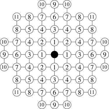
Consider a square lattice of size $L\times L$ with periodic boundary conditions. A lattice site may be occupied by utmost one particle. The first $k$ next nearest neighbors of a particle are excluded from being occupied by another particle. This corresponds to all lattice sites within a distance $R$ where $R^{2}$ is a positive integer. In Fig. 1, the sites excluded by a particle are shown for $k=1,2,\ldots,11$. For a given $k$, all sites with labels less than or equal to $k$ are excluded. An activity $z=\exp(\mu)$ is associated with each particle, where $\mu$ is the chemical potential.

Figure 1: The lattices sites that are excluded by a particle (black filled circle). The labels denote the sites that are the $k^{th}$ next nearest neighbors. For $k$-NN HCLG, all sites with labels less than or equal to $k$ are excluded.

We study this system using a grand canonical Monte Carlo algorithm. The algorithm is an adaptation of an efficient algorithm with cluster moves well suited to study hard core problems Kundu et al. (2012, 2013).

We describe the implementation of the algorithm for the 1-NN model and then outline the modifications required to implement it for larger $k$. Consider a valid configuration of the 1-NN model [see Fig. 2 (a)]. A row or column is chosen at random (say a row) and all particles on that row are removed. The aim is to reoccupy the row with a new configuration with the correct equilibrium weight. After evaporation, the row is divided by the excluded sites into intervals of contiguous empty sites [see Fig. 2 (b)]. In the 1-NN model, along a row, a particle excludes the nearest neighbor from being occupied by a particle. Thus, the particle configuration in an interval is independent of its neighboring intervals, and the re-occupation of the row reduces to the occupation of empty intervals.

Figure 2: The Monte Carlo algorithm illustrated for 1-NN. (a) A typical valid configuration. The lattice consists of particles (filled circles), excluded sites (empty circles) and empty sites where a particle may be added to obtain a new valid configuration. (b) A row is chosen at random (denoted by arrow) and all particles on that row are removed. The row is now divided into intervals of contiguous empty sites by the excluded sites. (c) The row is reoccupied with a new valid configuration with the correct equilibrium weight.

The calculation of probability of a configuration may be determined from the exact solution of the one dimensional problem on a lattice of length $l$ with open and periodic boundary conditions. Let $\Omega_{o}(z,\ell)$ [$\Omega_{p}(z,\ell)$] denote the partition function of the problem with nearest neighbor exclusion on a lattice with open [periodic] boundary conditions. They obey recursion relations

$$\Omega_{o}(z,\ell) = 1+\ell z(1-\delta_{\ell,0}),~{}\ell=0,\ldots,d,$$ (1a)

$$\Omega_{o}(z,\ell) = z\Omega(z,\ell-d-1)+\Omega(z,\ell-1),~{}\ell>d,$$ (1b)

$$\Omega_{p}(z,L) = dz\Omega_{o}(z,L-2d-1)+\Omega_{o}(z,L-d),$$ (1c)

where for the 1-NN model, $d=1$. Given an empty interval of length $\ell<L$, the probability that the left most site is occupied equals $z\Omega_{z,\ell-d}/\Omega_{\ell}$. If $\ell=L$, then the probability that one of the first $d$ sites is occupied equals $dz\Omega_{z,L-d-2}/\Omega_{p}(z,L)$. These probabilities are calculated for all $\ell$ and stored as input for the Monte Carlo simulations. A Monte Carlo step corresponds to $2L$ such evaporation–deposition moves. It is straightforward to show that the algorithm is ergodic and obeys detailed balance.

The algorithm is easily generalized to higher values of $k$. However, one cannot always choose rows and columns for the evaporation–deposition moves because the occupation of the empty intervals may no longer be independent of one another. This is most easily seen for the 3-NN model, where along a row, a particle excludes the nearest and next nearest neighbors. However, in a row, only one site is excluded by a particle that is two rows away. An example is shown in Fig. 3. A valid configuration is shown in Fig. 3(a). If a deposition is attempted in the row denoted by an arrow [see Fig. 3(b)], then the occupation of site A excludes site B which belongs to a different empty interval. This makes the occupation of different empty intervals interdependent. However, if one attempts evaporation and deposition along diagonals oriented in the $\pi/4$ direction [Fig. 3(c)], then the occupation of empty intervals become independent of each other. In Table 1, we tabulate the orientations of the diagonals for the evaporation–deposition moves that we have used for $k$ up to $k=11$. For each of these choices, the values of $d$ that should be used in Eq. (1) are also tabulated in Table 1.

Figure 3: An example of the algorithm for 3-NN. (a) A valid configuration of 2 particles (filled circles) and excluded sites (empty circles). (b) Adding particles in a row (denoted by arrow) by deposition. If a particle is added at A, then its exclusion range includes B. Thus, the occupation of the empty intervals are not independent. (c) Adding particles in a diagonal oriented in the $\pi/4$ direction (denoted by arrow). Now the occupation of the empty intervals are independent of each other.

Table 1: For each $k$, the orientation of the diagonals along which particles are evaporated and deposited, and the corresponding value of $d$ to be used in Eq. (1) are tabulated. Evaporation and deposition along diagonals separated by $\Delta$ or more are independent.

k	orientation of diagonal	d	$\Delta$
1	$0$, $\pi/2$	1	2
2	$0$, $\pi/2$	1	2
3	$\pi/4$, $3\pi/4$	1	3
4	$0$, $\pi/2$	2	3
5	$0$, $\pi/2$	2	3
6	$\tan^{-1}(\pm 2)$, $\tan^{-1}(\pm 1/2)$	1	7
7	$\pi/4$, $3\pi/4$	2	5
	$0$, $\pi/2$	3	4
8	$\pi/4$, $3\pi/4$	2	6
	$0$, $\pi/2$	3	4
9	$\pi/4$, $3\pi/4$	2	6
10	$\pi/4$, $3\pi/4$	2	6
11	$\tan^{-1}(\pm 2)$, $\tan^{-1}(\pm 1/2)$	1	10

We implement a parallel version of the above algorithm. The evaporation and deposition of particles in two rows in the 1-NN model (diagonals in general) that have at least $\Delta-1$ rows between them ($\Delta=2$ for the 1-NN model) are independent of each other. The value of $\Delta$ for different $k$ are given in Table 1. Hence, we update simultaneously every $\Delta$th row. Once all rows are updated in this manner, the columns are updated. The parallelization and efficiency of the algorithm allows us to simulate large system sizes and high densities.

We check for equilibration by initializing the simulations with two different initial configurations, corresponding to two different phases, and making sure that the final equilibrium state is independent of the initial condition. One configuration is a fully packed state and the other is a random configuration where particles are deposited at random.

In a typical run for a fixed value of $\mu$, after equilibration, the different thermodynamic quantities are averaged over $10^{8}$ Monte Carlo steps that are divided into 10 statistically independent blocks for estimating errors. In addition, we use the method of histogram re-weighting Ferrenberg and Swendsen (1988) to extrapolate for values of $\mu$ that are not directly simulated. This allows us to determine quantities like the maximum value of susceptibility and its location more precisely.

III Two transitions in the 4-NN model

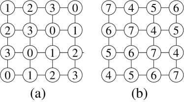
In this section, we show numerically that the 4-NN model undergoes two phase transitions with increasing density. To assist in defining the different phases, we divide the lattice into sublattices by assigning $2$ labels to each site. Each lattice site belongs to a diagonal oriented in the $\pi/4$ direction and to a diagonal oriented in the $3\pi/4$ direction. All sites that belong to a diagonal with orientation $\pi/4$ are assigned a label from $0$ to $3$ as shown in Fig. 4(a). If the coordinates of a site are $(x,y)$, then the label is $[(x-y)\mod 4]$. Similarly, all sites that belong to a diagonal with orientation $3\pi/4$ are assigned a label from $4$ to $7$ as shown in Fig. 4(b). If the coordinates of a site are $(x,y)$, then the label is $[(x+y)\mod 4+4]$.

Figure 4: The sublattice labeling for 4-NN. (a) All sites belonging to a diagonal oriented in the $\pi/4$ direction have same label. If the site has coordinates $(x,y)$, then the label is $[(x-y)\mod 4]$. (b) All sites belonging to a diagonal oriented in the $3\pi/4$ direction have same label. If the site has coordinates $(x,y)$, then the label is $[(x+y)\mod 4+4]$. In addition, all sites with label $0$ or $2$ (or equivalently $4$ and $6$) will be called sublattice $A$ and all sites with label $1$ or $3$ (or equivalently $5$ and $7$) will be called sublattice $B$.

Figure 5: Snapshots of typical configurations of the 4-NN model. The particles are colored according to the sublattice it belongs to (see Fig. 4). In the left panel, the colors are light blue for 0, dark magenta for 1, deep blue for 2 and plum for 3. In the right panel, the colors are dark green for 4, red for 5, light green for 6 and pink for 7. (a) Low density disordered phase where all four colors are present in both panels. (b) Intermediate density sublattice phase, where even or odd sublattices are preferentially occupied. (c) High density columnar phase, where one sublattice in one of the panels (left in figure) and two sublattices in the other panel are preferentially occupied.

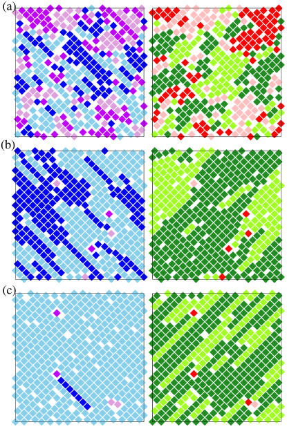
In Fig. 5, we show typical snapshots of the equilibrated system at low, intermediate and high densities. In the left panels, all particles belonging to sublattice $i$ ($i=0,1,2,3$) have the same color. Similarly, in the right panels, all particles belonging to sublattice $i$ ($i=4,5,6,7$) have the same color. At low densities [see Fig. 5(a)], all four colors are present (roughly equal) in both the left and right panels. This is the disordered phase with equal occupation of all sublattices $0,\ldots,7$. At intermediate densities [see Fig. 5(b)], we find that that majority of particles have two of the four colors in both left and right panels. This corresponds to particles preferably occupying either the even sublattices or the odd sublattices. There are two such states corresponding to particles in sublattices ($0,2$) and ($4,6$) or in sublattices ($1,3$) and ($5,7$). If we label the sites on sublattices $0$ and $2$ (equivalently $4$ and $6$) as $A$ and the sites on sublattices $1$ and $3$ (equivalently $5$ and $7$) as $B$, then this intermediate phase breaks the symmetry between $A$ and $B$ sublattices. We will call this phase a sublattice phase (following the terminology in Ref. Fernandes et al. (2007a)). We note that this phase was observed in Ref. Fernandes et al. (2007a). At high densities [see Fig. 5(c)], we find that the particles occupy one of the four sublattices from $0$–$3$ or $4$–$7$, but not from both. In the example shown in Fig. 5(c), in the left panel, particles preferentially occupy sublattice $0$. However, in the right panel, particles occupy mostly two sublattices ($4$ and $6$). This phase is identical to the high density phase of the hard square model (2-NN) where there is positional order in one direction but no positional order in the perpendicular direction due to a sliding instability. We call this phase the columnar phase. There are $8$ such states, corresponding to the number of sublattices.

To distinguish between phases quantitatively, we define two order parameters $Q_{sl}$ and $Q_{cl}$, where $sl$ denotes sublattice and $cl$ denotes columnar. Let $\rho_{i}$, $i=0,\ldots,7$ be the density of particles in sublattice $i$. We define

$$Q_{sl} = \lvert(\rho_{0}+\rho_{2})-(\rho_{1}+\rho_{3})\rvert,$$ (2a)

$$Q_{cl} = \lvert\sum_{k=0}^{3}\rho_{k}e^{ik\pi/2}\rvert-\lvert\sum_{k=4}^{7}\rho_{k}e^{ik\pi/2}\rvert.$$ (2b)

$Q_{sl}$ measures the difference between the densities of sublattices $A$ (sites in even sublattices) and $B$ (sites in odd sublattices). It is zero in the disordered phase and non-zero in both the sublattice and columnar phases. $Q_{cl}$ is zero in both the disordered and sublattice phases and non-zero only in the columnar phase.

Figure 6: (Color online) The variation of the order parameters $Q_{sl}$ and $Q_{cl}$ with chemical potential $\mu$ for different system sizes $L$. $Q_{sl}$ becomes non-zero at a smaller value of $\mu$ than $Q_{cl}$.

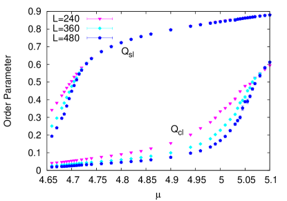
While the snapshots in Fig. 5 are indicative of two transitions, we now show unambiguously the existence of two transitions. Figure 6 shows the variation of the two order parameters with chemical potential. Clearly, $Q_{sl}$ takes on a $L$ independent non-zero value when the chemical potential is larger than $\mu\approx 4.70$ ($\rho\approx 0.110$). At this value of $\mu$ $Q_{cl}$ is still zero. $Q_{cl}$ takes on a $L$ independent non-zero value when the chemical potential is larger than $\mu\approx 5.07$ ($\rho\approx 0.116$). The two values of $\mu$ being clearly different, we conclude that there are two transitions.

The other thermodynamic quantities of interest are the susceptibility $\chi$, the second moment of the order parameter $\chi^{(2)}$, the Binder cumulant $U$, and compressibility $\kappa$, defined as

$$\chi = L^{2}[\langle Q^{2}\rangle-\langle Q\rangle^{2}],$$ (3a)

$$\chi^{(2)} = L^{2}\langle Q\rangle^{2},$$ (3b)

$$U = 1-\frac{\langle Q^{4}\rangle}{3\langle Q^{2}\rangle^{2}},$$ (3c)

$$\kappa = L^{2}[\langle\rho^{2}\rangle-\langle\rho\rangle^{2}],$$ (3d)

where Q represent Q_sl or Q_cl. Though $\chi$ and $\chi^{(2)}$ resemble each other, we find that the data for $\chi^{(2)}$ is much cleaner. The nature of the phase transitions is determined by the singular behavior of $U$, $Q$, $\chi$, and $\chi^{(2)}$ near the critical point. Let $\epsilon=(\mu-\mu_{c})/\mu_{c}$, where $\mu_{c}$ is the critical chemical potential. The singular behavior is characterized by the critical exponents $\nu,$ $\beta$, $\gamma$, and $\alpha$ defined by $Q\sim(-\epsilon)^{\beta}$, $\epsilon<0$, $\chi\sim|\epsilon|^{-\gamma}$, $\chi^{(2)}\sim|\epsilon|^{-\gamma}$, $\kappa\sim|\epsilon|^{-\alpha}$and $\xi\sim|\epsilon|^{-\nu}$, where $\xi$ is the correlation length and $|\epsilon|\rightarrow 0$. The other critical exponents may be obtained from scaling relations. The exponents are obtained by finite size scaling of the different quantities near the critical point:

$$U \simeq f_{U}(\epsilon L^{1/\nu}),$$ (4a)

$$Q \simeq L^{-\beta/\nu}f_{Q}(\epsilon L^{1/\nu}),$$ (4b)

$$\chi \simeq L^{\gamma/\nu}f_{\chi}(\epsilon L^{1/\nu}),$$ (4c)

$$\chi^{(2)} \simeq L^{\gamma/\nu}f^{(2)}_{\chi}(\epsilon L^{1/\nu}),$$ (4d)

$$\kappa \simeq L^{\alpha/\nu}f_{\kappa}(\epsilon L^{1/\nu}),$$ (4e)

where $f_{U}$, $f_{Q}$, $f_{\chi}$, $f^{(2)}_{\chi}$, $f_{\kappa}$ are scaling functions and the system size is $L\times L$. In addition, if $\chi$ has a maximum $\chi_{max}(L)$ at $\mu_{c}(L)$, then

$$\chi_{max}(L) \propto L^{\gamma/\nu},$$ (5a)

$$\mu_{c}(L)-\mu_{c}(\infty) \propto L^{-1/\nu}.$$ (5b)

Figure 7: (Color online) The data for cumulants of $Q_{sl}$ for the 4-NN model near the first transition from the disordered phase to sublattice phase. (a) The Binder cumulant $U_{sl}$ for different L intersect at $\mu_{c}=4.705$. The data for (b) $U_{sl}$, (c) $Q_{sl}$, and (d) $\chi_{sl}^{(2)}$ for different $L$ collapse onto a single curve when scaled as in Eq. (4) with the Ising exponents $\beta/\nu=1/8$, $\gamma/\nu=7/4$, and $\nu=1$. (e) The variation of the maximum value $\chi_{max}$ of the susceptibility $\chi$ with $L$. The solid line is a best fit to the data with slope $\gamma/\nu=1.72\pm 0.04$. (f) The variation of the order parameter $Q_{sl}$ at the critical point with $L$. The solid line is a best fit to the data with slope $-\beta/\nu=-0.136\pm 0.017$. (g) Variation of $\mu_{c}$ for different $L$ with $1/L$. The straight line intersects the $\mu$-axis at $\mu_{c}=4.705\pm 0.005$. (h) The variation of the compressibility $\kappa$ at the critical point with $L$. The straight line shows $\kappa(\mu_{c})\sim\ln L$.

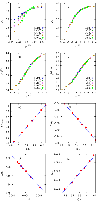
The first transition from disordered to sublattice phase was studied in Ref. Fernandes et al. (2007a) using system sizes varying from $L=80$ to $L=240$, and was argued to be in the Ising universality class. However, analysis of the cluster integrals predict non-Ising exponents Rotman and Eisenberg (2009). We re-examine this transition with data for system sizes up to $L=600$. In addition to obtaining better estimates of the critical exponents, it also acts as a check for our Monte Carlo algorithm. The data for the different thermodynamic quantities near the disordered-sublattice transition are shown in Fig. 7. The critical chemical potential $\mu_{c}$ is obtained from the intersection of the curves for the Binder cumulant $U_{sl}$ for different system sizes. The intersection point depends very weakly on $L$ [see Fig. 7(a)] allowing for an accurate determination of $\mu_{c}$. We thus obtain $\mu_{c}=4.705\pm 0.005$, consistent with the $\mu_{c}$ found in Ref. Fernandes et al. (2007a). In the disordered-sublattice transition, the system breaks the symmetry between $A$ and $B$ sublattices. Due to the two-fold symmetry, we expect this transition to be in universality class of the two dimensional Ising model. Indeed, we find excellent data collapse when the data for $U_{sl}$ [see Fig. 7(b)], $Q_{sl}$ [see Fig. 7(c)] and $\chi_{sl}^{(2)}$ [see Fig. 7(d)] are scaled as in Eq. (4) with Ising exponents $\beta/\nu=1/8$, $\gamma/\nu=7/4$ and $\nu=1$.

We also estimate $\beta/\nu$ and $\gamma/\nu$ independently. The maximum value of susceptibility $\chi_{max}$ scales with $L$ as $L^{\gamma/\nu}$. We calculate $\chi_{max}$ by the method of histogram re-weighting, and obtain $\gamma/\nu=1.72\pm 0.04$ [Fig. 7(e)]. The order parameter $Q_{sl}$ at the critical point decreases with $L$ as $L^{-\beta/\nu}$. By simulating for different $L$, we obtain $\beta/\nu=0.136\pm 0.017$ [see Fig. 7(f)]. Both these numerical values are consistent with the Ising exponents. In Fig. 7(g), we show the variation of $\mu_{c}(L)$ with $1/L$. The data lie on a straight line, consistent with $\nu=1$. The intersection of the straight line with the $\mu$-axis gives $\mu_{c}=4.705\pm 0.005$, consistent with the estimation from the crossing of the curves for the Binder cumulant. Finally, we examine the data for compressibility $\kappa$ at the critical point. The data for compressibility is more noisy that that for other quantities, but is consistent with a logarithmic divergence with $L$ [see Fig. 7(h)], as expected for the Ising universality class. Thus, we conclude, as in Ref. Fernandes et al. (2007a) and contrary to the conclusion in Ref. Rotman and Eisenberg (2009), that the transition from disordered to sublattice phase is in the Ising universality class,

We now focus on the second transition from the sublattice phase to the columnar phase. Suppose, in the sublattice phase, the system is in sublattice $A$. This corresponds to all sites belonging to sublattices $0,2,4,6$. In the second transition, the system picks out one of the four sublattices, with equal occupation of two other sublattices. Since this transition breaks a four fold symmetry, we expect this transition, if continuous, to be in the universality class of the two color Ashkin Teller model. We, thus, expect $\gamma/\nu=7/4$, $\beta/\nu=1/8$, and $\nu$ depending on the parameters of the problem at hand Baxter (1982). We now provide numerical evidence of the same.

Figure 8: (Color online) The data for cumulants of $Q_{cl}$ for the 4-NN model near the second transition from the sublattice phase to the columnar phase. (a) The Binder cumulant $U_{cl}$ for different $L$ intersect at $\mu_{c}=5.07\pm 0.01$. The data for (b) $U_{cl}$, (c) $Q_{sl}$ and (d) $\chi_{sl}^{(2)}$ for different $L$ collapse onto a single curve when scaled as in Eq. (4) with critical exponents $\beta/\nu=1/8$, $\gamma/\nu=7/4$ and $\nu=0.83\pm 0.06$. (e) The variation of the maximum value $\chi_{max}$ of the susceptibility $\chi$ with $L$. The solid line is a best fit to the data with slope $\gamma/\nu=1.76\pm 0.05$. (f)The variation of the order parameter $Q_{sl}$ at the critical point with $L$. The solid line is a best fit to the data with slope $-\beta/\nu=-0.113\pm 0.015$. (g) Variation of $\mu_{c}$ for different $L$ with $L^{-1/\nu}$. The straight line intersects $\mu$-axis at $\mu_{c}=5.066\pm 0.01$. (h) The variation of compressibility $\kappa$ at the critical point $\mu_{c}$ with $L$. The solid line is a best fit to the data with slope $\alpha/\nu=-0.34\pm 0.08$.

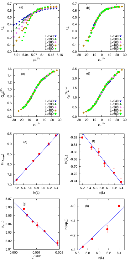
The data for the different thermodynamic quantities for the second transition are shown in Fig. 8. From the intersection of the curves of $U_{cl}$ for different $L$ [see Fig. 8(a)], we obtain $\mu_{c}=5.07\pm 0.01$. The Binder cumulant data for different system sizes collapse onto a single curve when scaled as in Eq. (4a) with $\nu=0.083\pm 0.06$ [see Fig. 8(b)]. For this value of $\nu$ and $\gamma/\nu=7/4$, $\beta/\nu=1/8$, we obtain excellent data collapse for $Q_{sl}$ [see Fig. 8(c)] and $\chi_{sl}^{(2)}$ [see Fig. 8(d)] when scaled as in Eq. (4b) and Eq. (4c) respectively. Thus, we conclude that the transition belongs to the Ashkin Teller universality class with $\nu=0.83\pm 0.06$, lying between the $4$ state Potts and Ising points. Independent measurement of $\gamma/\nu$ from the variation of the maximum of susceptibility with $L$ gives $\gamma/\nu=1.76\pm 0.05$ [see Fig. 8(e)]. Similarly, from the dependence of $Q_{sl}$ on $L$ at the critical point, we obtain $\beta/\nu=0.113\pm 0.015$ [see Fig. 8(f)]. Both these values are consistent with the Ashkin Teller universality class. In Fig.  8(g), we show the dependence of the critical chemical potential $\mu_{c}(L)$ on $L$. When plotted against $L^{-1/\nu}$ [see Eq. (5b)], with $\nu=0.83$, the data lie on a straight line which intersects the $\mu$-axis at $\mu_{c}=5.066\pm 0.01$. This estimate of the critical $\mu$ is consistent with the value obtained from the intersection of the curves for the Binder cumulants. Since $\nu<1$, the exponent $\alpha>0$ and we expect the compressibility $\kappa$ to diverge at the critical point with exponent $\alpha/\nu$. The data for $\kappa$ is very noisy [see Fig. 8(h)] when compared to data for other thermodynamic quantities. Fitting to a power law, we obtain $\alpha/\nu=0.34\pm 0.08$ . Within error bars, $\alpha/\nu$ satisfies the exponent equality $2\nu=2-\alpha$.

We conclude that the 4-NN model, contrary to what was known earlier, undergoes two entropy driven transitions with increasing density. In order to provide some understanding of this phenomena, we derive the high density expansion of the model in the next section.

IV High density expansion of the 4-NN model

In this section, we calculate the first four terms in the large $z$ (high density) expansion of the free energy for the 4-NN model. We show that the high density phase (say all particles in mostly sublattice $0$) has a sliding instability only for defects in sublattice $2$ and not for defects in sublattices $1$ and $3$. This results in the densities of defects in the different sublattices being different at large $z$. We argue that this sliding instability could be the origin of the two phase transitions in the 4-NN model.

The high density phase of the 4-NN model being columnar, the high density expansion is very similar to that for the 2-NN model Bellemans and Nigam (1967); Ramola and Dhar (2012). Due to the sliding instability, the large $z$ expansion of the 2-NN model is in powers of $1/\sqrt{z}$ instead of the usual $1/z$ Mayer series. The first three terms in the high density expansion for the 2-NN model was obtained in Ref. Bellemans and Nigam (1967). More recently, it has been systematically extended to $4$ terms Ramola and Dhar (2012). We will closely follow the calculations of Ref. Ramola and Dhar (2012), modifying when necessary for the 4-NN model.

Consider a fully packed configuration of the 4-NN model. It has density $1/8$. If the particles occupy one of the sublattice from $0$ to $3$, then they occupy two sublattices from $4$ to $7$ and vice-versa (see Fig. 4 for labeling of sublattices). For example, if the particles are all in sublattice $0$, then they are also simultaneously in sublattices $4$ and $6$. It is easy to see that the number of fully packed configurations is $8(2^{L/2}-1)$, where we assume that $L$ is even. Though the degeneracy diverges with $L$, the entropy per unit site is zero in the thermodynamic limit.

For constructing the large $z$ expansion, we will describe the lattice sites only in terms of sublattices $0$ to $3$. Let the activities on sublattice $i$ be $z_{i}$. We will consider $z_{0}\gg z_{i}$, $i=1,2,3$. After the expansion is obtained, we will equate all the activities to $z$. Thus, it will be an expansion about an ordered state where all the particles are in sublattice $0$. The free energy $f(z_{0},z_{1},z_{2},z_{3})$ is defined as

$$f(z_{0},z_{1},z_{2},z_{3})=\lim_{N\rightarrow\infty}\frac{-1}{N}\ln\mathcal{L}(z_{0},z_{1},z_{2},z_{3}),$$ (6)

where $\mathcal{L}(z_{0},z_{1},z_{2},z_{3})$ is the grand canonical partition function. To lowest order, the contribution to the partition function is $\mathcal{L}(z_{0},0,0,0)$. It is easy to see that the partition function breaks up into a product of one dimensional partition functions, and is

$$\mathcal{L}(z_{0},0,0,0)=\Omega_{p}(z_{0},L)^{L/4}.$$ (7)

Here $\Omega_{p}(z,\ell)$ and $\Omega_{o}(z,\ell)$ are the partition functions of a nearest neighbor exclusion hard core gas on a one dimensional lattice of length $\ell$ with periodic and open boundary conditions respectively, as defined in Eq. (1) with $d=1$.

Solving Eq. (1), we obtain Bellemans and Nigam (1967); Ramola and Dhar (2012)

$$\Omega_{o}(z,\ell) = \frac{\lambda_{+}^{\ell+2}-\lambda_{-}^{\ell+2}}{\sqrt{1+4z}},~{}\ell=0,1,\ldots,$$ (8)

$$\Omega_{p}(z,\ell) = \lambda_{+}^{\ell}+\lambda_{-}^{\ell},~{}\ell=2,3,\ldots,$$ (9)

where

$$\lambda_{\pm}=\frac{1\pm\sqrt{1+4z}}{2}.$$ (10)

Knowing the partition functions, the contribution from configurations with zero defects (all particles in sublattice $0$) to the free energy is

$$f(z_{0},0,0,0)=\frac{-\ln z_{0}}{8}-\frac{1}{8\sqrt{z_{0}}}+\frac{1}{192z_{0}^{3/2}}+O(\frac{1}{z_{0}^{5/2}}).$$ (11)

We now switch on $z_{1}$. This creates some defect sites in sublattice $1$. We first calculate the contribution from configurations with a single defect. A single defect on sublattice $1$ excludes $4$ sites from the diagonal of sublattice $0$ closest to it and 2 sites from the diagonal further away from it [see Fig. 9(a)]. The contribution of configurations with one defect to the partition function is

$$\left.\frac{\mathcal{L}(z_{0},z_{1},0,0)}{\mathcal{L}(z_{0},0,0,0)}\right|_{1D}=\frac{Nz_{1}}{4}\frac{\Omega_{o}(z_{0},L-4)\Omega_{o}(z_{0},L-2)}{\Omega_{p}(z_{0},L)^{2}},$$ (12)

where the factor $N/4$ is the number of ways of placing a particle on sublattice $1$, and $1D$ denotes one defect. Expanding for large $z_{0}$, we obtain

$$\left.\frac{\mathcal{L}(z_{0},z_{1},0,0)}{\mathcal{L}(z_{0},0,0,0)}\right|_{1D}=Nz_{1}\left[\frac{1}{16z_{0}^{2}}-\frac{1}{16z_{0}^{5/2}}+O(z_{0}^{-3})\right].$$ (13)

Figure 9: Examples of one and two defect configurations on sublattices $1$ and $3$ for an ordered state where particles are on sublattice $0$. Black circles are particles, empty and lightly shaded circles are excluded sites. Exclusions only on sublattice $0$ are shown in (a)–(c) and (e). $0,1,2,3$ denote the diagonals that belong to sublattices $0,1,2,3$. (a) A single defect on sublattice $1$. (b) Two defects on sublattice $1$ but on neighboring diagonals. A and B are two other lattice sites where the defect may be placed. (c) Two defects on sublattice $1$ but on the same diagonal. (d) A defect on sublattice $1$ and a defect on sublattice $3$ at one of the $4$ closest positions. The empty circles are all the excluded sites due to defect on sublattice $1$ while the lightly shaded circles are excluded sites on sublattice $0$ due to defect on sublattice $3$. (e) A defect on sublattice $1$ and a defect on sublattice $3$ positioned such that they exclude the same two sites on the diagonal $0$ separating them.

We now consider the contribution from configurations with two defects on sublattice $1$. The lowest order contributions come from the two defects being on the same diagonal or on adjacent diagonals. First consider two defects on adjacent diagonals, as shown in Fig. 9(b). Now, $4$, $4$ and $2$ lattice sites are excluded from diagonals belonging to sublattice $0$. The ratio of the partition functions with $z_{1}\neq 0$ and $z_{1}=0$ for this configuration with two defects is

$$\frac{3Nz_{1}^{2}}{4}\frac{\Omega_{o}(z_{0},L-4)^{2}\Omega_{o}(z_{0},L-2)}{\Omega_{p}(z_{0},L)^{3}},$$ (14)

where the factor $3N/4$ is the combinatorial factor associated with the number of ways of placing the pair of particles. For each choice of the position of the first particle ($N/4$ ways), there are 3 ways of placing the second particle (A, B, and filled circle). Expanding for large $z_{0}$, we obtain

$$Nz_{1}^{2}\left[\frac{3}{32z_{0}^{7/2}}+O(z_{0}^{-4})\right].$$ (15)

Second, consider the case when two defects are on sublattice $1$ but on the same diagonal, as shown in Fig. 9(c). Now, $6$ and $4$ lattice sites are excluded from diagonals belonging to sublattice $0$. The ratio of the partition functions for this two defect configuration is

$$\frac{Nz_{1}^{2}}{4}\frac{\Omega_{o}(z_{0},L-6)\Omega_{o}(z_{0},L-4)}{\Omega_{p}(z_{0},L)^{2}},$$ (16)

where the factor $N/4$ is the combinatorial factor associated with the number of ways of placing the pair of particles. Expanding for large $z_{0}$, we obtain

$$Nz_{1}^{2}O(z_{0}^{-4}).$$ (17)

Thus, to order $z^{-3/2}$, there is no contribution. Collecting together the terms, we obtain

$$\left.\frac{\mathcal{L}(z_{0},z_{1},0,0)}{\mathcal{L}(z_{0},0,0,0)}\right|_{2D}=Nz_{1}^{2}\left[\frac{3}{32z_{0}^{7/2}}+O(z_{0}^{-3})\right].$$ (18)

It is straightforward to verify that the contribution from configurations with $3$ defects do not contribute to terms up to order $z^{-3/2}$.

We now switch on a small $z_{3}$. Sublattices $1$ and $3$ being symmetric with respect to sublattice $0$, the contribution from configurations with a single defect on sublattice $3$ is identical to Eq. (13) except for $z_{1}\to z_{3}$. Similarly, configurations with two defects on sublattice $3$ have the same contribution as Eq. (18) with $z_{1}\to z_{3}$. We now calculate the contribution to the partition function from configurations with one defect on sublattice $1$ and another on sublattice $3$ as shown in Fig. 9(d) and (e). In Fig. 9(d), the particles are placed as close to each other as possible. Given a particle on sublattice $1$ (placed in $N/4$ ways), there are four ways of placing a particle on sublattice $3$. The ratio of the partition functions for this two defect configuration is

$$Nz_{1}z_{3}\frac{\Omega_{o}(z_{0},L-2)^{2}\Omega_{o}(z_{0},L-6)}{\Omega_{p}(z_{0},L)^{3}}.$$ (19)

Expanding for large $z_{0}$, we obtain

$$Nz_{1}z_{3}\left[\frac{1}{8z_{0}^{7/2}}+O(z_{0}^{-4})\right].$$ (20)

Now, consider the configuration shown In Fig. 9(e). Once the first particle is placed (in $N/4$ ways), there is a unique position for the second particle. The ratio of partition functions when two such defects are present is

$$\frac{Nz_{1}z_{3}}{4}\frac{\Omega_{o}(z_{0},L-4)^{2}\Omega_{o}(z_{0},L-2)}{\Omega_{p}(z_{0},L)^{3}}.$$ (21)

Expanding for large $z_{0}$, we obtain

$$Nz_{1}z_{3}\left[\frac{1}{32z_{0}^{7/2}}+O(z_{0}^{-4})\right].$$ (22)

Combining together the contributions from configurations with one or two defects on sublattices $1$ and $3$, we obtain

$$\frac{\mathcal{L}(z_{0},z_{1},0,z_{3})}{\mathcal{L}(z_{0},0,0,0)}=N(z_{1}+z_{3})\left[\frac{1}{16z_{0}^{2}}-\frac{1}{16z_{0}^{5/2}}\right]$$

$$+\frac{3N(z_{1}^{2}+z_{3}^{2})}{32z_{0}^{7/2}}+\frac{5Nz_{1}z_{3}}{32z_{0}^{7/2}}+O(z^{-2}).$$ (23)

We now focus on defects in sublattice $2$. Unlike defects in sublattices $1$ and $3$, a vacancy on sublattice $0$ can be broken into two half vacancies with the points in between being defects on sublattice $2$. Thus, $n$ defects on sublattice $2$ contribute at the same order as a single defect Ramola and Dhar (2012). The expansion is better performed in terms of rods which are a collection of contiguous defects in the $3\pi/4$ direction on sublattice $2$ Ramola and Dhar (2012). An example of a rod of length $3$ is shown in Fig. 10 (focus only on black circles and empty circles that are triplets). It excludes three sites each from $4$ diagonals belonging to sublattice $0$. It is straightforward to obtain the contribution from a single rod Ramola and Dhar (2012):

$$\left.\frac{\mathcal{L}(z_{0},0,z_{2},0)}{\mathcal{L}(z_{0},0,0,0)}\right|_{1R} = \frac{N}{4}\sum_{n=1}^{\infty}z_{2}^{n}\left[\frac{\Omega_{o}(z_{0},L-3)}{\Omega_{p}(z_{0},L)}\right]^{n+1},$$ (24a)

$$= \frac{N}{4}\frac{z_{2}\beta^{2}}{1-z_{2}\beta},$$ (24b)

where $1R$ denoted one rod and

$$\beta=\frac{1}{\sqrt{1+4z_{0}}\lambda_{+}},$$ (25)

is a function only of $z_{0}$.

Figure 10: Example of a rod-like defect on sublattice $2$ and defects on sublattice $1$. Black circles are particles on sublattice $2$. Empty circles are excluded sites on sublattice $0$ or sublattice $1$ (all not shown) due to defect on sublattice $2$. Lightly shaded circles are excluded sites due to defects at $A$ or $C$. Circles with a pattern are excluded sites due to defect at $B$.

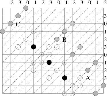
The calculation of the contribution from two rods on sublattice $2$ is identical to that for the 2-NN model, except for an overall factor of $1/2$ due to only half the lattice sites being involved in the calculation. Thus, one can read off the results from the calculations of Ref. Ramola and Dhar (2012) for the 2-NN model.

A further contribution to the free energy at order $z^{-3/2}$ is due to configurations with a rod on sublattice $2$ and a particle on sublattice $1$ or $3$. Given a rod on sublattice $2$, there are three kinds of sites on sublattice $1$ where a particle may be placed. These are denoted by $A$, $B$ and $C$ (see Fig. 10). The contribution to the ratios of partition functions $\mathcal{L}(z_{0},z_{1},z_{2},0)/\mathcal{L}(z_{0},0,0,0)$ for the different cases are

$$A : \frac{N}{4}z_{2}^{n}\left[\frac{\Omega_{o}(z_{0},L-3)}{\Omega_{p}(z_{0},L)}\right]^{n}$$ (26)

$$\times 2z_{1}\frac{\Omega_{o}(z_{0},L-5)\Omega_{o}(z_{0},L-2)}{\Omega_{p}(z_{0},L)^{2}}\sim O(z^{-3/2}),$$

$$B : \frac{N}{4}z_{2}^{n}\left[\frac{\Omega_{o}(z_{0},L-3)}{\Omega_{p}(z_{0},L)}\right]^{n-1}$$ (27)

$$\times 2nz_{1}\frac{\Omega_{o}(z_{0},L-6)\Omega_{o}(z_{0},L-5)}{\Omega_{p}(z_{0},L)^{2}}\sim O(z^{-5/2}),$$

$$C : \frac{N}{4}z_{2}^{n}\left[\frac{\Omega_{o}(z_{0},L-3)}{\Omega_{p}(z_{0},L)}\right]^{n}$$ (28)

$$\times 2z_{1}\frac{\Omega_{o}(z_{0},L-4)}{\Omega_{p}(z_{0},L)}\sim O(z^{-3/2}),$$

where $n$ is the length of the rod. Thus to order $z^{-3/2}$, only cases $A$ and $C$ are relevant, and their contribution to the free energy add up to

$$\left.\frac{\mathcal{L}(z_{0},z_{1},z_{2},z_{3})}{\mathcal{L}(z_{0},0,0,0)}\right|_{1R,1D}=\frac{N}{4}\frac{z_{2}\beta}{1-z_{2}\beta}\frac{(z_{1}+z_{3})}{2z_{0}^{5/2}}$$

$$+\frac{N}{4}\frac{z_{2}\beta^{2}}{1-z_{2}\beta}\frac{(z_{1}+z_{3})}{z_{0}^{3/2}}+O(z^{-2}),$$ (29)

where, in the right hand side of Eq. (IV), the first term is due to $A$ and the second term is due to $C$.

The free energy of the 4-NN model may now be written down up to $O(z^{-3/2})$. In terms of the partition functions,

$$f(z_{0},z_{1},z_{2},z_{3})=-\frac{\ln\mathcal{L}(z_{0},0,0,0)}{N}-\frac{\mathcal{L}(z_{0},z_{1},z_{2},z_{3})}{N\mathcal{L}(z_{0},0,0,0)}.$$ (30)

Adding the contribution from configurations with two rods, as obtained in Ref. Ramola and Dhar (2012), to Eqs. (11), (IV), (24b), and (IV), and equating $z_{i}=z$, we obtain

$$-f(z)=\frac{1}{8}\ln z+\frac{1}{8z^{1/2}}+\frac{1}{4z}+\frac{\frac{3}{2}\ln\frac{9}{8}+\frac{149}{192}}{z^{3/2}}+O(z^{-2}).$$ (31)

Knowing the free energy, the particle densities in each sublattice is given by $\rho_{i}=z_{i}\partial/\partial z_{i}(-f)$. Doing the algebra and simplifying,

$$\rho(z) = \frac{1}{8}-\frac{1}{16z^{1/2}}-\frac{1}{4z}-\frac{\frac{9}{4}\ln\frac{9}{8}+\frac{149}{128}}{z^{3/2}}+O(\frac{1}{z^{2}}),$$ (32)

$$\rho_{0}(z) = \frac{1}{8}-\frac{1}{16z^{1/2}}-\frac{5}{8z}-\frac{\frac{605}{128}+\frac{17}{4}\ln\frac{9}{8}}{z^{3/2}}+O(\frac{1}{z^{2}}),$$ (33)

$$\rho_{1}(z) = \frac{1}{16z}+\frac{17}{32z^{3/2}}+O(\frac{1}{z^{2}}),$$ (34)

$$\rho_{2}(z) = \frac{1}{4z}+\frac{2\ln\frac{9}{8}+\frac{5}{2}}{z^{3/2}}+O(\frac{1}{z^{2}}).$$ (35)

Figure 11: (Color online) Variation of the densities of particles in different sublattices, truncated at order $z^{-3/2}$ [see Eqs. (33), (34), (35)], with $1/z$.

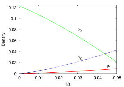
The sublattice densities, truncated at order $z^{-3/2}$ are plotted in Fig. 11. Clearly, due to the sliding instability, the density on sublattice $2$ increases faster than that of sublattices $1$ and $3$. Equating $\rho_{0}$ and $\rho_{2}$ in Eqs. (33) and (35), an estimate of the critical activity may be estimated. We find $z_{c}=22.742\ldots$ or $\mu_{c}=3.1242\ldots$. This should be compared with the actual value of $\mu_{c}\approx 5.07$.

The faster increase in the particle density of the sublattice where sliding instability exists is the likely reason for the second transition. As density is increased, the system is first destabilized by the sliding instability into sublattices $0$ and $2$. This is followed by a second transition where the density of sublattices $1$, $3$ equals that of $0$, $2$.

V Multiple transitions in the $k$-NN HCLG

In this section, we generalize the arguments of Sec. IV to larger $k$. We ask for a criteria that will help determine whether the HCLG for a given $k$ will undergo multiple transitions. From the analysis of the 4-NN model, it is clear that if the high density phase is columnar, then it is easier to generate defects in the sublattices where the sliding instability is present as compared to other sublattices. Hence, we conjecture that if the model satisfies (i) the high density phase is columnar and (ii) the sliding instability is present in only a fraction of the sublattices, then the system will show multiple transitions.

Figure 12: One of the configurations of maximum density for different $k$. Particles are shown by large filled circles. The excluded sites are shown by small circles. A circle that encloses the excluded sites due to a particle are drawn around the left most and top most particles. The empty large circles denote sites that may be occupied by sliding all particles on that diagonal, keeping other particles fixed. The examples are for (a) 6-NN, (b) 7-NN, (c) 8-NN, (d) 9-NN, (e) 10-NN, and (f) 11-NN.

In hard square systems ($k=2,5$), though the high density phase is columnar, the sliding instability is along all sublattices and hence does not satisfy condition (ii). Hence, one expects only one transition for the hard square system, at least for $2\times 2$ and $3\times 3$ systems. Models, other than hard square models, that show columnar order at high densities will typically have sliding instability in only a few sublattices. For $k>5$, none of the $k$-NN HCLG models are hard square models. Thus, the criteria reduces to determining whether the high density phase is columnar or not.

The nature of the phase at high densities may be determined by constructing configurations at full packing for different $k$. In Fig. 12, we show configurations at full packing for $k=6$ to $11$. In each of the plots, $4$ particles (filled circles) that constitute the unit cell are shown. A circle of radius $R$, which depends on $k$, is drawn around two of these particles – the left most and top most. $R$ is distance of the farthest exclusion point from the particle hence all lattice sites within or on the circle are excluded by the particle. The value of $R$ for different $k$ is given in Table. 2. In all the cases, the configuration can be thought of as particles placed on equidistant parallel diagonals (not necessarily oriented in the $\pi/4$ direction). In some cases [see Fig. 12 (e) and (f)], all the particles in a diagonal may be slid by one or two lattice spacings without affecting the configurations in other diagonals. Such allowed sites are denoted by empty large circles. If such a freedom to slide exists, the system will have columnar order at high densities.

Table 2: For each $k$, the square of radius of circle of exclusion $R^{2}$, density at full packing $\rho_{max}$ and the nature of the high density phase are tabulated.

k	$R^{2}$	$\rho_{max}$	High density phase
1	1	1/2	Sublattice
2	2	1/4	Columnar
3	4	1/5	Sublattice
4	5	1/8	Columnar
5	8	1/9	Columnar
6	9	1/10	Sublattice
7	10	1/12	Sublattice
8	13	1/15	Sublattice
9	16	1/15	Sublattice
10	17	1/18	Columnar
11	18	1/20	Columnar
12	20	1/23	Sublattice
13	25	1/24	Sublattice
14	26	1/28	Columnar

For 6-NN, in the fully packed configuration, the particles are along diagonals oriented in the $\tan^{-1}(1/3)$ or $\tan^{-1}(3)$ directions [see Fig. 12(a)]. There is no freedom to slide, and hence we expect sublattice order at full packing. This is true for $k=7,8,9$, where the diagonals are oriented in different directions for different $k$ [see Fig. 12(b)–(d)]. Thus, the conjecture would predict a single first order transition to an ordered sublattice phase for $k=6,\ldots,9$.

For the 10-NN model, the particles in any diagonal may be slid by one or two lattice sites in the $\pi/4$ direction without affecting the configurations in the other diagonals [see Fig. 12(e)]. For the 11-NN model, all the particles in a diagonal may be slid by one lattice spacing in the $\tan^{-1}(1/2)$ direction without affecting the configurations in the other diagonals [see Fig. 12(f)]. Thus, the conjecture predicts that there should be multiple transitions in the 10-NN and 11-NN model.

The analysis is easily extended to larger $k$ by constructing the fully packed configurations. For instance, the next $k$ to have columnar order at high densities is $k=14$. The nature of the high density phase and the density at full packing for $k\leq 14$ are summarized in Table. 2.

VI Monte Carlo simulations for $k=6,\ldots,11$

In this section, we present results from Monte Carlo simulations for $k$-NN HCLG models with $k=6,\ldots,11$ to verify the conjecture presented in Sec. V. We refer to Sec. II and Table 1 for details of the simulations. We present the details for $k=6$ to $k=9$ in Sec. VI.1, $k=10$ is Sec. VI.2, $k=11$ in Sec. VI.3.

VI.1 The 6-NN to 9-NN models

The conjecture in Sec. V predicts a single first order transition from a disordered phase to an ordered sublattice phase for $k=6,7,8,9$. In order to define suitable order parameters, we divide the lattice sites into different sublattices. Like in the 4-NN model, each site belongs to two sublattices.

The sublattices for the 6-NN model are shown in Fig. 13. In Fig. 13(a) [Fig. 13(b)], all sites belonging to a diagonal oriented in the $\tan^{-1}(1/3)$ [$\tan^{-1}(3)$] direction belong to the same sublattice. There are $10$ sublattices each for the two choices. In the high density phase, most particles will occupy one of the $20$ sublattices with maximum density $1/10$.

Figure 13: The sublattices of the 6-NN model. (a) All sites on a diagonal oriented in the $\tan^{-1}(1/3)$ direction belong to the same sublattice. (b) All sites on a diagonal oriented in the $\tan^{-1}(3)$ direction belong to the same sublattice.

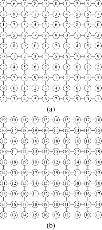
The sublattices for the 7-NN model are shown in Fig. 14. In Fig. 14(a) [Fig. 14(b)], all sites belonging to a diagonal oriented in the $\tan^{-1}(2/3)$ [$\tan^{-1}(3/2)$] direction belong to the same sublattice. There are $12$ sublattices each for the two choices. In the high density phase, most particles will occupy one of the $24$ sublattices with maximum density $1/12$.

Figure 14: The sublattices of the 7-NN model. (a) All sites on a diagonal oriented in the $\tan^{-1}(2/3)$ direction belong to the same sublattice. (b) All sites on a diagonal oriented in the $\tan^{-1}(3/2)$ direction belong to the same sublattice.

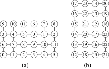
The sublattices for the 8-NN model are shown in Fig. 15. In Fig. 15(a) [Fig. 15(b)], all sites belonging to a diagonal oriented in the $\tan^{-1}(1/4)$ [$\tan^{-1}(-4)$] direction belong to the same sublattice. There are $15$ sublattices each for the two choices. In the high density phase, most particles will occupy one of the $30$ sublattices with maximum density $1/15$.

Figure 15: The sublattices of the 8-NN and the 9-NN models. (a) All sites on a diagonal oriented in the $\tan^{-1}(1/4)$ direction belong to the same sublattice. (b) All sites on a diagonal oriented in the $\tan^{-1}(-4)$ direction belong to the same sublattice.

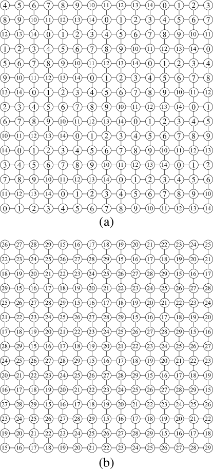
The sublattices for the 9-NN model are identical to that for the 8-NN model shown in Fig. 15, and hence maximum density will be $1/15$.

To study the phase transition into the sublattice phase for $k=6$ to $9$, we define an order parameter

$$Q_{k}=\lvert Q_{k}^{(a)}\rvert-\lvert Q_{k}^{(b)}\rvert,$$ (36)

where $k=6,7,8,9$ denotes k-NN and $Q_{k}^{(a)}$ and $Q_{k}^{(b)}$ measure sublattice ordering according to the sublattice labeling in (a) and (b) respectively of Figs. 13, 14, and 15 and are defined as

$$Q_{k}^{(a)} = \sum_{j=0}^{m-1}\rho_{j}e^{2\pi\iota j/m},$$ (37)

$$Q_{k}^{(b)} = \sum_{j=m}^{2m-1}\rho_{j}e^{2\pi\iota j/m}.$$ (38)

Here $\rho_{j}$ is the particle density in sublattice $j$. The parameter $m$ depends on $k$ and has values $10$ (6-NN), $12$ (7-NN), $15$ (8-NN) and $15$ (9-NN). Clearly, $Q_{i}$ is zero in the disordered phase and non-zero in the sublattice ordered phase.

We now study the transitions for $k=6$ to $k=9$ using the above order parameter. To show that a transition is first order, we measure the probability density function (pdf) of the density $\rho$ and order parameter $Q_{k}$ near the transition for two different values of $L$. The pdfs should have two peaks that do not move closer to each other with increasing $L$. One of the peaks correspond to the disordered phase and the other to the ordered phase. This will be taken as a signature of a first order transition.

We observe transitions at critical chemical potentials $\mu_{c}\approx 4.66$ ($k=6$), $\mu_{c}\approx 4.88$ ($k=7$), $\mu\approx 6.07$ ($k=8$), and $\mu\approx 4.63$ ($k=9$). Surprisingly, we find $\mu_{c}$ for 9-NN to be smaller than that for 6-NN.

Figure 16: (Color online) The probability density function for density $\rho$ (left panels) and order parameter $Q_{k}$ (right panels) for $\mu\approx\mu_{c}$, the critical chemical potential, for two different system sizes. The data are for the k-NN model with $k=6$ [(a) and (b)], $k=7$ [(c) and (d)], $k=8$ [(e) and (f)], and $k=9$ [(g) and (h)].

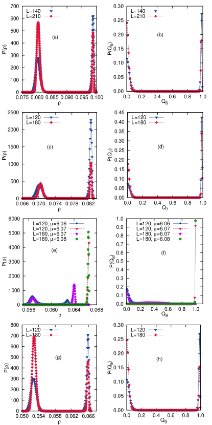
The pdfs for $\rho$ and $Q_{k}$ are shown in Fig. 16 (a), (b) [6-NN], (c), (d) [7-NN], (e), (f) [8-NN] and (g), (h) [9-NN]. In all the plots, we observe that the pdfs have two peaks that do not approach each with increasing system size. For 8-NN [see Fig. 16 (e), (f)], there is a long-lived metastable state at a density that lies between those for the low-disordered phase and the high-density sublattice phase. Hence, the pdf for $\mu>\mu_{c}$ is peaked at a value different from the peak at the transition point. We, therefore, conclude that the transitions in the 6-NN to 9-NN models are first order.

We check that the phase for values of $\mu\lesssim\mu_{c}$ is the disordered phase and for values of $\mu\gtrsim\mu_{c}$ is the sublattice ordered phase (by looking at typical snapshots) expected at full packing. Thus, we do not expect any more transitions. Both the first order nature and the single transition are consistent with the conjecture in Sec. V.

VI.2 The 10-NN model

For the 10-NN model, the conjecture in Sec. V predicts multiple transitions. In this subsection, we confirm the same. We divide the lattice into sublattices as shown in Fig. 17. Each site belongs to two sublattices. In Fig. 17(a) [Fig. 17(b)], all sites belonging to a diagonal oriented in the $\pi/4$ ($3\pi/4$) direction belong to the same sublattice. There are $6$ sublattices each for the two choices.

Figure 17: The sublattices of the 10-NN model. (a) All sites on a diagonal oriented in the $\pi/4$ direction belong to the same sublattice. (b) All sites on a diagonal oriented in the $3\pi/4$ direction belong to the same sublattice.

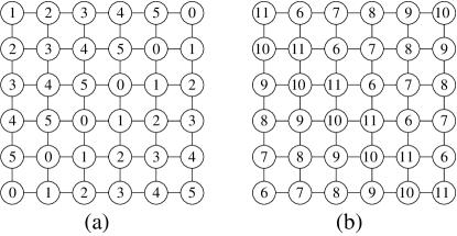
In the high density phase, we expect the system to be in a columnar phase where all the particles occupy one sublattice either from $0$ to $5$ or from $6$ to $11$. For example, if the particles are all in sublattice $0$ direction, they are also in sublattices $6$, $8$ and $10$. The maximum density possible is $1/18$.

We first show that, if all the particles are in sublattice $0$ in the columnar phase, then there is a sliding instability along sublattices $2$ and $4$. To do so, we consider configurations with defects on sublattice $2$ or sublattice $4$ that are rod-like, and show that rods of all lengths contribute at same order. In Fig. 18, we show examples of configurations with rods of length $3$ on sublattice $2$ (black circles) and on sublattice $4$ (lightly shaded circles). A rod of length $n$ excludes $5$ sites each from $n+1$ diagonals belonging to sublattice $0$. The contribution from configurations with rods of length $n$ to the ratio of partition functions $\mathcal{L}(z_{0},0,z_{2},0,0,0/\mathcal{L}(z_{0},0,0,0,0,0)$ configuration is

$$\frac{N}{6}z_{2}^{n}\left[\frac{\Omega_{o}(z_{0},L-5)}{\Omega_{p}(z_{0},L)}\right]^{n+1}.$$ (39)

In the 10-NN model, along a diagonal, a particle excludes its nearest and next-nearest neighbors from being occupied by a particle. Then, to leading order $\Omega_{o}(z_{0},L-5)\sim z_{0}^{L/3-1}$, and $\Omega_{p}(z_{0},L)\sim z_{0}^{L/3}$. Thus, the term in Eq. (39) is $z^{-1}$ to leading order for all $n\geq 1$.

Figure 18: An example of rod-like defects of length $3$ on sublattices $2$ (black circles) or $4$ (grey circles) in the 10-NN model. Exclusions only on sublattice $0$ are shown by empty circles. $0,1,2,3,4,5$ on the edge of the box denote diagonals that belong to sublattices $0,1,2,3,4,5$ respectively.

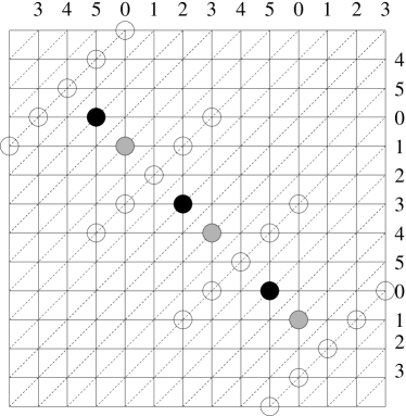
Thus, the sliding instability exists along sublattices $2$ and $4$. It is straightforward to verify that it does not exist on sublattices $1$, $3$, and $5$. The conjecture in Sec. V then predicts that as $z$ is decreased, the columnar phase should first destabilize into a phase where particle densities will be equal on all even sublattices and all odd sublattices, but not equal to each other. If we label the even sublattices as $A$ and odd sublattices as $B$, then there is a symmetry breaking between $A$ and $B$. Further decrease in $z$ would result in a disordered phase. Like for the 4-NN model, we will call the intermediate phase as a sublattice phase.

In terms of increasing $z$ or $\mu$, we expect the first transition to be in the universality class of two dimensional Ising model because of symmetry breaking between two symmetric phases. In the second transition, the system chooses from one of $6$ symmetric phases. By analogy with Potts model, we expect the second transition to be first order.

We now confirm these predictions numerically. To study the first transition, we define an order parameter,

$$Q_{1}=\lvert(\rho_{0}+\rho_{2}+\rho_{4})-(\rho_{1}+\rho_{3}+\rho_{5})\rvert,$$ (40)

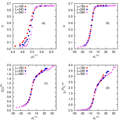
where $\rho_{i}$ are the particle densities on sublattice $i$. $Q_{1}$ measures the density difference between even and odd sublattices. The data for the different thermodynamic quantities near the disordered-sublattice transition are shown in Fig. 19. The critical chemical potential $\mu_{c}$ is obtained from the intersection of the Binder cumulant curves $U_{1}$ for different system sizes. We obtain $\mu_{c}=5.3\pm 0.05$. The data for $U_{1}$ [see Fig. 19(b)], $Q_{1}$ [see Fig. 19(c)] and $\chi_{1}^{(2)}$ [see Fig. 19(d)] for different system sizes collapse onto a single curve when scaled as in Eq. (4) with Ising exponents $\beta/\nu=1/8$, $\gamma/\nu=7/4$ and $\nu=1$. These results confirm that the first transition is continuous and is consistent to the Ising universality class.

Figure 19: (Color online) The data for cumulants of $Q_{1}$ for the 10-NN model near the first transition from the disordered phase to sublattice phase. (a) The Binder cumulant $U_{1}$ for different L crosses at $\mu_{c}=5.30$. The data for (b) $U_{1}$, (c) $Q_{1}$, and (d) $\chi_{1}^{(2)}$ for different $L$ collapse onto a single curve when scaled as in Eq. (4) with the Ising exponents $\beta/\nu=1/8$, $\gamma/\nu=7/4$, and $\nu=1$.

Figure 20: (Color online) The probability density function for (a) density $\rho$ and (b) order parameter $Q_{10}$ near the transition point ($\mu_{c}\approx 6.0$) for three different system sizes. The data are for the 10-NN model.

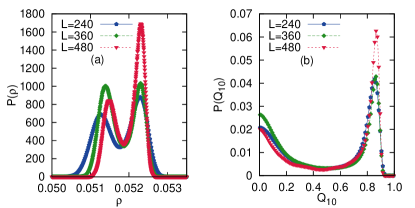
We now study the second transition. This is best done using an order parameter $Q_{10}$ as defined in Eqs. (36) and (37) with $m=6$ in Eq. (37). $Q_{10}$ is zero in disordered and sublattice phases and non-zero in the columnar phase. We find that $Q_{10}$ is zero for $\mu\lesssim 5.95$ and non zero for $\mu\gtrsim 6.00$. These values are distinctly larger than the critical chemical potential found above for the first transition ($5.30$). To establish the first order nature of the transition, we measure the pdfs of density $\rho$ and $Q_{10}$ near the transition point. These are shown in Fig. 20 (a) and (b). The pdfs for both quantities have two well separated peaks that become sharper with increasing system size. This is a clear signature of a first order transition.

We check that the phase for values of $\mu\gtrsim\mu_{c}$ is the columnar ordered phase (by looking at typical snapshots) expected at full packing. Thus, we do not expect any more transitions. Thus, the numerical data are consistent with the conjecture in Sec. V.

VI.3 The 11-NN model

For the 11-NN model, the conjecture in Sec. V predicts multiple transitions. In this subsection, we numerically confirm the same. We divide the lattice into sublattices as shown in Fig. 21. In contrast to sublattice decomposition for $k\leq 10$, now each site belongs to four sublattices. In Fig. 17(a), (b), (c), and (d), all sites belonging to a diagonal oriented in the $\tan^{-1}(1/2)$, $\tan^{-1}(-1/2)$, $\tan^{-1}(2)$, and $\tan^{-1}(-2)$ directions respectively belong to the same sublattice. There are $10$ sublattices for each of the four choices.

Figure 21: The sublattices of the 11-NN model. (a) All sites on a diagonal oriented in the $\tan^{-1}(1/2)$ direction belong to the same sublattice. (b) All sites on a diagonal oriented in the $\tan^{-1}(-1/2)$ direction belong to the same sublattice. (c) All sites on a diagonal oriented in the $\tan^{-1}(2)$ direction belong to the same sublattice. (b) All sites on a diagonal oriented in the $\tan^{-1}(-2)$ direction belong to the same sublattice.

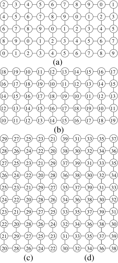
In the high density phase, we expect the system to be in a columnar phase where all the particles occupy one sublattice chosen from one of the sets $0$ to $9$, $10$ to $19$, $20$ to $29$, and $30$ to $39$. An example of a columnar phase would be all particles in sublattice $0$. In that case, the particles are also simultaneously in all even sublattices between $10$ and $19$, all sublattices between $20$ and $29$, and sublattices $30$ and $35$. Along a diagonal in sublattice $0$, there is nearest neighbor exclusion. Hence, the maximum density possible is $1/20$.

Consider, now, the high density phase. Suppose the ordered phase is one in which all particles are present in sublattice $0$. We now introduce defects and ask what sublattices have a sliding instability. We skip the details, but it is straightforward to verify that the sliding instability is present only for sublattice $5$. This means that $n$-rod defects of $n$ defects on sublattice $5$ contribute to the same order in the free energy. The conjecture in Sec. V therefore predicts that the high density phase should destabilize into a phase where two sublattices are equally occupied. Further decrease in chemical potential would finally result in a low density disordered phase.

We now present results from Monte Carlo simulations for the 11-NN model. As chemical potential is increased, we find that the system undergoes a first order transition (see below) at $\mu_{c}\approx 6.40$. However, for $\mu\gtrsim\mu_{c}$, the phase that we observe is not the phase where $2$ sublattices are present. Instead, we observe a phase in which particles are mostly present on even sublattices (for e.g., 0,2,4,6,8) or odd sublattices (for e.g.,1,3,5,7,9). Equivalently, in terms of rows and columns, the particles occupy every fourth row or every fourth column. There are $8$ such states.

A convenient order parameter to study the transition is

$$Q_{11}=\lvert\sum_{j=0}^{3}r_{j}e^{2\pi\iota j/4}\rvert-\lvert\sum_{j=0}^{3}c_{j}e^{2\pi\iota j/4}\rvert$$ (41)

where $r_{j}$ is the particle density in rows $[j\mod 4]$ and $c_{j}$ is the particle density in columns $[j\mod 4]$. $Q_{11}$ is zero in the disordered phase and non-zero in the intermediate phase.

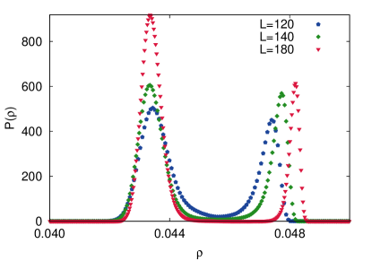
We first show that the density $\rho$ has a discontinuity across the transition. In Fig. 22, we show the pdf for $\rho$ for three different system sizes near the transition point. The pdfs have two distinctly separated peaks that sharpen with system size. This is a clear indication of a first order transition.

Figure 22: (Color online) The probability distribution function for density $\rho$ near the transition point for three different system sizes. The data are for the 11-NN model.

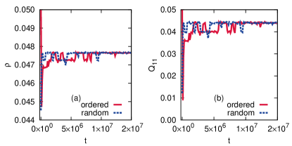
The densities above the transition are very close to the maximum density possible ($1/20$). Since there is a possibility that the system may not have equilibrated, we present evidence for equilibration. The variation of density $\rho$ and the order parameter $Q_{11}$ with time is shown in Fig. 23. The data are for two different initial conditions. In the first, the initial configuration is one of maximal density, where all particles are on sublattice $0$. In the second, the initial configuration is a random one where $10^{5}$ deposition attempts (singe particle) are made at random locations. We find that, though the time profiles for the two initial conditions are different, they are statistically identical for larger times (see Fig. 23(a) for $\rho$ and (b) for $Q_{11}$. Further, we also check using snapshots that the long time behavior for both initial conditions is one every fourth row or column are occupied. We, thus, conclude that the system is equilibrated in our simulations.

Figure 23: (Color online) The variation of (a) density $\rho$ and (b) order parameter $Q_{11}$ with time $t$ for the 11-NN model when $\mu\gtrsim\mu_{c}$. The data are for two different initial conditions. In the first, labelled “ordered”, all particles are in sublattice $0$. In the second, labelled “random”, particles are initially deposited at random.

The intermediate phase, being different from the fully packed phase, we expect at least one more transition. But our conjecture in Sec. V predicts the existence of a phase where two sublattices are occupied. If this conjecture is true, then we expect at least two more transitions with increasing $\mu$. Unfortunately, within available computational time, we are unable to equilibrate the system for larger $\mu$, and hence unable to verify the above claim.

VII Summary and conclusions

In this paper, we revisited the well-studied two-dimensional $k$-NN hard core lattice gas model, where the first $k$ next nearest neighbors of a particle are excluded from being occupied by another particle. Using an efficient Monte Carlo algorithm, we were able to study numerically systems with $k$ up to $11$, earlier studies having been limited to $k\leq 5$. Surprisingly, we found that systems with certain $k$ ($k=4,10,11,\ldots$) undergo multiple entropy driven transitions with increasing density. That these models may show multiple transitions have not be appreciated in the literature hitherto. For the 4-NN model, the presence of two transitions resolved an existing puzzle as to why the system had a continuous transition when analogy with the Potts model predicted a first order transition. In this paper, we showed that the 8-fold symmetry is broken in two steps leading to two continuous transitions – one belonging to the Ising universality class and the other to the two color Ashkin Teller universality class – rather than a single first order transition. To rationalize this finding, we studied analytically the 4-NN model using a large $z$ expansion. The high density phase being columnar, the expansion is in powers of $1/\sqrt{z}$ rather than the usual Mayer expansion in $1/z$. From the first four terms of the expansion, it was shown that the densities of defects increases more rapidly in sublattices where a sliding instability is present when compared to sublattices where it is absent. This led us to conjecture that if the high density phase is columnar and the system is not a hard square system, then the model should show multiple transitions. This conjecture predicts single first order transitions for $k=6,7,8,9$, and multiple transitions for $k=10,11$. This claim was verified numerically.

In particular, for the 10-NN model, we showed that there are two transitions. The first transition into a sublattice phase is continuous and is indistinguishable from the Ising universality class. The second transition is first order. For the 11-NN model, due to computational limitations, we were able to numerically study only the first transition. However, the intermediate ordered phase was shown to be different from the phase at full packing. Hence, at least one more transition will definitely be present. Surprisingly, we found the intermediate phase to be different from what we found for the 4-NN and 10-NN models. For these latter models, as $z$ is decreased from infinity, the system first destabilizes into a state where the original sublattice and sublattices with sliding instability are present, consistent with our conjecture. Hence, we expect the 11-NN model to undergo at least three transitions with increasing density.

It would be interesting to verify the above claim for 11-NN. Unfortunately, we are unable to equilibrate the 11-NN system at densities higher than just beyond the first transition. Seeking improvements to the algorithm in the future may help. One possible direction would be to use flat histogram Monte Carlo algorithms like the the Wang-Landau algorithm Wang and Landau (2001a, b) or tomographic sampling Dickman and Cunha-Netto (2011); Belardinelli et al. (2014). A different approach would be to calculate the high density expansion for the densities of particles in different sublattices for the 10-NN and 11-NN models. Like in the 4-NN model, this will help to identify the preferred sublattices for generation of defects.

For the 4-NN model, by simulating systems up to $L=600$ (earlier simulations Fernandes et al. (2007a) having studied $L=240$), we confirm that the first transition from the low density disordered phase to the intermediate sublattice phase is indistinguishable from the universality class of the two-dimensional Ising model. However, sophisticated analysis based on cluster integrals rule out Ising universality class Rotman and Eisenberg (2009). This cluster analysis works very well for other repulsive interaction models and is a promising tool for studying phase transitions. It would therefore be important to understand why it fails for the 4-NN model. In particular should the analysis be modified in the presence of multiple transitions?

Explaining the transitions in the $k$-NN models by analytical methods is an open problem. Possible approaches include modified Flory approximation Fernandes et al. (2007b) and fundamental measure theory Lafuente and Cuesta (2003a, b); Schmidt et al. (2003) that have been applied earlier to HCLG models like the 2-NN model. Reproducing the two transitions in the 4-NN model would be a test for efficacy of these theories. A different approach would be to look for exact solutions for arbitrary $k$ on simpler lattices like the random lattice or the Bethe lattice where the solution of the 1-NN model is known Runnels (1967), or the recently introduced random locally tree like layered lattice Dhar et al. (2011); Kundu and Rajesh (2013). A precise formulation of what extended hard core exclusion range means on these lattices will be the first step. Also, to the best of our knowledge, unlike the sublattice phase, there is no rigorous proof for the existence of columnar phase for any model. The large $z$ expansions for the 2-NN model Bellemans and Nigam (1967); Ramola and Dhar (2012); Ramola (2012) and the 4-NN model in this paper are only heuristic evidence for the existence of the columnar phase. In a recent paper, the existence of a nematic phase with orientational ordering was proved in Ref. Disertori and Giuliani (2013). It would be interesting to see if such methods can be extended to prove the existence of columnar phase.

The algorithm used in the paper is well suited to efficiently study hard core exclusion models on other lattices, dimensions, and for particles of different shapes. In three dimensions, simulations of hard cubes in the continuum show a first order transition from a disordered phase to a simple cubic crystal phase Smallenburg et al. (2012). It would be interesting to study the lattice version of the hard cube model as well as the k-NN model in three dimensions, and obtain the phase diagram. Another interesting problem is that of rounded squares in two dimensions. Recent experiments on brownian squares report the existence of hexagonal, rhombic and square phases Zhao et al. (2011). Some of these features have been reproduced in simulations of rounded squares Avendaño and Escobedo (2012); Carmichael and Shell (2013). It is straightforward to make a lattice version of such shapes, making it suitable to be studied by our algorithm. These are promising areas for future study.