Conditional Density Estimation
with Dimensionality Reduction via
Squared-Loss Conditional Entropy Minimization

Abstract

Regression aims at estimating the conditional mean of output given input. However, regression is not informative enough if the conditional density is multimodal, heteroscedastic, and asymmetric. In such a case, estimating the conditional density itself is preferable, but conditional density estimation (CDE) is challenging in high-dimensional space. A naive approach to coping with high-dimensionality is to first perform dimensionality reduction (DR) and then execute CDE. However, such a two-step process does not perform well in practice because the error incurred in the first DR step can be magnified in the second CDE step. In this paper, we propose a novel single-shot procedure that performs CDE and DR simultaneously in an integrated way. Our key idea is to formulate DR as the problem of minimizing a squared-loss variant of conditional entropy, and this is solved via CDE. Thus, an additional CDE step is not needed after DR. We demonstrate the usefulness of the proposed method through extensive experiments on various datasets including humanoid robot transition and computer art.

Keywords: Conditional density estimation, dimensionality reduction

1 Introduction

Analyzing input-output relationship from samples is one of the central challenges in machine learning. The most common approach is regression, which estimates the conditional mean of output $\boldsymbol{y}$ given input $\boldsymbol{x}$. However, just analyzing the conditional mean is not informative enough, when the conditional density $p(\boldsymbol{y}|\boldsymbol{x})$ possesses multimodality, asymmetry, and heteroscedasticity (i.e., input-dependent variance) as a function of output $\boldsymbol{y}$. In such cases, it would be more appropriate to estimate the conditional density itself (Figure 2).

The most naive approach to conditional density estimation (CDE) would be $\epsilon$-neighbor kernel density estimation ($\epsilon$-KDE), which performs standard KDE along $\boldsymbol{y}$ only with nearby samples in the input domain. However, $\epsilon$-KDE do not work well in high-dimensional problems because the number of nearby samples is too few. To avoid the small sample problem, KDE may be applied twice to estimate $p(\boldsymbol{x},\boldsymbol{y})$ and $p(\boldsymbol{x})$ separately and the estimated densities may be plugged into the decomposed form $p(\boldsymbol{y}|\boldsymbol{x})=p(\boldsymbol{x},\boldsymbol{y})/p(\boldsymbol{x})$ to estimate the conditional density. However, taking the ratio of two estimated densities significantly magnifies the estimation error and thus is not reliable. To overcome this problem, an approach to directly estimating the density ratio $p(\boldsymbol{x},\boldsymbol{y})/p(\boldsymbol{x})$ without separate estimation of densities $p(\boldsymbol{x},\boldsymbol{y})$ and $p(\boldsymbol{x})$ has been explored (Sugiyama et al., 2010). This method, called least-squares CDE (LSCDE), was proved to possess the optimal non-parametric learning rate in the mini-max sense, and its solution can be efficiently and analytically computed. Nevertheless, estimating conditional densities in high-dimensional problems is still challenging.

A natural idea to cope with the high-dimensionality is to perform dimensionality reduction (DR) before CDE. Sufficient DR (Li, 1991; Cook and Ni, 2005) is a framework of supervised DR aimed at finding the subspace of input $\boldsymbol{x}$ that contains all information on output $\boldsymbol{y}$, and a method based on conditional-covariance operators in reproducing kernel Hilbert spaces has been proposed (Fukumizu et al., 2009). Although this method possesses superior thoretical properties, it is not easy to use in practice because no systematic model selection method is available for kernel parameters. To overcome this problem, an alternative sufficient DR method based on squared-loss mutual information (SMI) has been proposed recently (Suzuki and Sugiyama, 2013). This method involves non-parametric estimation of SMI that is theoretically guaranteed to achieve the optimal estimation rate, and all tuning parameters can be systematically chosen in practice by cross-validation with respect to the SMI approximation error.

Given such state-of-the-art DR methods, performing DR before LSCDE would be a promising approach to improving the accuracy of CDE in high-dimensional problems. However, such a two-step approach is not preferable because DR in the first step is performed without regard to CDE in the second step and thus small error incurred in the DR step can be significantly magnified in the CDE step.

In this paper, we propose a single-shot method that integrates DR and CDE. Our key idea is to formulate the sufficient DR problem in terms of the squared-loss conditional entropy (SCE) which includes the conditional density in its definition, and LSCDE is executed when DR is performed. Therefore, when DR is completed, the final conditional density estimator has already been obtained without an additional CDE step (Figure 1). We demonstrate the usefulness of the proposed method, named least-squares conditional entropy (LSCE), through experiments on benchmark datasets, humanoid robot control simulations, and computer art.

(a) CDE without DR

(b) CDE after DR

(c) CDE with DR (proposed)

Figure 1: Conditional density estimation (CDE) and dimensionality reduction (DR). (a) CDE without DR performs poorly in high-dimensional problems. (b) CDE after DR can magnify the small DR error in the CDE step. (c) CDE with DR (proposed) performs CDE in the DR process in an integrated manner.

2 Conditional Density Estimation with Dimensionality Reduction

In this section, we describe our proposed method for conditional density estimation with dimensionality reduction.

2.1 Problem Formulation

Let $\mathcal{D}_{\textbf{x}}(\subset\mathbb{R}^{d_{\textbf{x}}})$ and $\mathcal{D}_{\textbf{y}}(\subset\mathbb{R}^{d_{\textbf{y}}})$ be the input and output domains with dimensionality $d_{\textbf{x}}$ and $d_{\textbf{y}}$, respectively, and let $p(\boldsymbol{x},\boldsymbol{y})$ be a joint probability density on $\mathcal{D}_{\textbf{x}}\times\mathcal{D}_{\textbf{y}}$. Assume that we are given $n$ independent and identically distributed (i.i.d.) training samples from the joint density:

$$\{(\boldsymbol{x}_{i},\boldsymbol{y}_{i})\}_{i=1}^{n}\stackrel{{\scriptstyle\mathrm{i.i.d.}}}{{\sim}}p(\boldsymbol{x},\boldsymbol{y}).$$

The goal is to estimate the conditional density $p(\boldsymbol{y}|\boldsymbol{x})$ from the samples.

Our implicit assumption is that the input dimensionality $d_{\textbf{x}}$ is large, but its “intrinsic” dimensionality, denoted by $d_{\textbf{z}}$, is rather small. More specifically, let $\boldsymbol{W}$ and $\boldsymbol{W}_{\perp}$ be $d_{\textbf{z}}\times d_{\textbf{x}}$ and $(d_{\textbf{x}}-d_{\textbf{z}})\times d_{\textbf{x}}$ matrices such that $\begin{bmatrix}\boldsymbol{W}^{\top},\boldsymbol{W}_{\perp}^{\top}\end{bmatrix}$ is an orthogonal matrix. Then we assume that $\boldsymbol{x}$ can be decomposed into the component $\boldsymbol{z}=\boldsymbol{W}\boldsymbol{x}$ and its perpendicular component $\boldsymbol{z}_{\perp}=\boldsymbol{W}_{\perp}\boldsymbol{x}$ so that $\boldsymbol{y}$ and $\boldsymbol{x}$ are conditionally independent given $\boldsymbol{z}$:

$$\boldsymbol{y}\mathchoice{\mathrel{\hbox to0.0pt{$\displaystyle\perp$\hss}\mkern 2.0mu{\displaystyle\perp}}}{\mathrel{\hbox to0.0pt{$\textstyle\perp$\hss}\mkern 2.0mu{\textstyle\perp}}}{\mathrel{\hbox to0.0pt{$\scriptstyle\perp$\hss}\mkern 2.0mu{\scriptstyle\perp}}}{\mathrel{\hbox to0.0pt{$\scriptscriptstyle\perp$\hss}\mkern 2.0mu{\scriptscriptstyle\perp}}}\boldsymbol{x}|\boldsymbol{z}.$$ (1)

This measn that $\boldsymbol{z}$ is the relevant part of $\boldsymbol{x}$, and the rest $\boldsymbol{z}_{\perp}$ does not contain any information on $\boldsymbol{y}$. The problem of finding $\boldsymbol{W}$ is called sufficient dimensionality reduction (Li, 1991; Cook and Ni, 2005).

2.2 Sufficient Dimensionality Reduction with SCE

Let us consider a squared-loss variant of conditional entropy named squared-loss CE (SCE):

$$\mathrm{SCE}(\boldsymbol{Y}|\boldsymbol{Z}) =-\frac{1}{2}\iint\Big{(}p(\boldsymbol{y}|\boldsymbol{z})-1\Big{)}^{2}p(\boldsymbol{z})\mathrm{d}\boldsymbol{z}\mathrm{d}\boldsymbol{y}.$$ (2)

By expanding the squared term in Eq.(2), we obtained

$$\mathrm{SCE}(\boldsymbol{Y}|\boldsymbol{Z}) =-\frac{1}{2}\iint p(\boldsymbol{y}|\boldsymbol{z})^{2}p(\boldsymbol{z})\mathrm{d}\boldsymbol{z}\mathrm{d}\boldsymbol{y}+\iint p(\boldsymbol{y}|\boldsymbol{z})p(\boldsymbol{z})\mathrm{d}\boldsymbol{z}\mathrm{d}\boldsymbol{y}-\frac{1}{2}\iint p(\boldsymbol{z})\mathrm{d}\boldsymbol{z}\mathrm{d}\boldsymbol{y}$$

$$=-\frac{1}{2}\iint p(\boldsymbol{y}|\boldsymbol{z})^{2}p(\boldsymbol{z})\mathrm{d}\boldsymbol{z}\mathrm{d}\boldsymbol{y}+1-\frac{1}{2}\int\mathrm{d}\boldsymbol{y}$$

$$=\widetilde{\mathrm{SCE}}(\boldsymbol{Y}|\boldsymbol{Z})+1-\frac{1}{2}\int\mathrm{d}\boldsymbol{y},$$ (3)

where $\widetilde{\mathrm{SCE}}(\boldsymbol{Y}|\boldsymbol{Z})$ is defined as

$$\widetilde{\mathrm{SCE}}(\boldsymbol{Y}|\boldsymbol{Z}) =-\frac{1}{2}\iint p(\boldsymbol{y}|\boldsymbol{z})^{2}p(\boldsymbol{z})\mathrm{d}\boldsymbol{z}\mathrm{d}\boldsymbol{y}.$$ (4)

Then we have the following theorem (its proof is given in Appendix A), which forms the basis of our proposed method:

Theorem 1.

$$\widetilde{\mathrm{SCE}}(\boldsymbol{Y}|\boldsymbol{Z})-\widetilde{\mathrm{SCE}}(\boldsymbol{Y}|\boldsymbol{X}) =\frac{1}{2}\iint\left(\frac{p(\boldsymbol{z}_{\perp},\boldsymbol{y}|\boldsymbol{z})}{p(\boldsymbol{z}_{\perp}|\boldsymbol{z})p(\boldsymbol{y}|\boldsymbol{z})}-1\right)^{2}p(\boldsymbol{y}|\boldsymbol{z})^{2}p(\boldsymbol{x})\mathrm{d}\boldsymbol{x}\mathrm{d}\boldsymbol{y}$$

$$\geq 0.$$

This theorem shows $\widetilde{\mathrm{SCE}}(\boldsymbol{Y}|\boldsymbol{Z})\geq\widetilde{\mathrm{SCE}}(\boldsymbol{Y}|\boldsymbol{X})$, and the equality holds if and only if

$$p(\boldsymbol{z}_{\perp},\boldsymbol{y}|\boldsymbol{z})=p(\boldsymbol{z}_{\perp}|\boldsymbol{z})p(\boldsymbol{y}|\boldsymbol{z}).$$

This is equivalent to the conditional independence (1), and therefore sufficient dimensionality reduction can be performed by minimizing $\widetilde{\mathrm{SCE}}(\boldsymbol{Y}|\boldsymbol{Z})$ with respect to $\boldsymbol{W}$:

$$\boldsymbol{W}^{*}=\mathop{\mathrm{argmin}}_{\boldsymbol{W}\in\mathbb{G}_{d_{\textbf{z}}}^{d_{\textbf{x}}}(\mathbb{R})}\widetilde{\mathrm{SCE}}(\boldsymbol{Y}|\boldsymbol{Z}=\boldsymbol{W}\boldsymbol{X}).$$ (5)

Here, $\mathbb{G}_{d_{\textbf{z}}}^{d_{\textbf{x}}}(\mathbb{R})$ denotes the Grassmann manifold, which is a set of orthogonal matrices without overlaps:

$$\mathbb{G}_{d_{\textbf{z}}}^{d_{\textbf{x}}}(\mathbb{R})=\{\boldsymbol{W}\in\mathbb{R}^{d_{\textbf{z}}\times d_{\textbf{x}}}\ |\ \boldsymbol{W}\boldsymbol{W}^{\top}=\boldsymbol{I}_{d_{\textbf{z}}}\}/\sim,$$

where $\boldsymbol{I}$ denotes the identity matrix and $\sim$ represents the equivalence relation: $\boldsymbol{W}$ and $\boldsymbol{W}^{\prime}$ are written as $\boldsymbol{W}\sim\boldsymbol{W}^{\prime}$ if their rows span the same subspace.

Since $p(\boldsymbol{y}|\boldsymbol{z})=p(\boldsymbol{z},\boldsymbol{y})/p(\boldsymbol{z})$, $\mathrm{SCE}(\boldsymbol{Y}|\boldsymbol{Z})$ is equivalent to the negative Pearson divergence (Pearson, 1900) from $p(\boldsymbol{z},\boldsymbol{y})$ to $p(\boldsymbol{z})$, which is a member of the $f$-divergence class (Ali and Silvey, 1966; Csiszár, 1967) with the squared-loss function. On the other hand, ordinary conditional entropy (CE), defined by

$$\mathrm{CE}(\boldsymbol{Y}|\boldsymbol{Z})=-\iint p(\boldsymbol{z},\boldsymbol{y})\log p(\boldsymbol{y}|\boldsymbol{z})\mathrm{d}\boldsymbol{z}\mathrm{d}\boldsymbol{y},$$

is the negative Kullback-Leibler divergence (Kullback and Leibler, 1951) from $p(\boldsymbol{z},\boldsymbol{y})$ to $p(\boldsymbol{z})$. Since the Kullback-Leibler divergence is also a member of the $f$-divergence class (with the log-loss function), CE and SCE have similar properties. Indeed, the above theorem also holds for ordinary CE. However, the Pearson divergence is shown to be more robust against outliers (Sugiyama et al., 2012), since the log function—which is very sharp near zero—is not included. Furthermore, as shown below, $\widetilde{\mathrm{SCE}}$ can be approximated analytically and thus its derivative can also be easily computed. This is a critical property for developing a dimensionality reduction method because we want to minimize $\widetilde{\mathrm{SCE}}$ with respect to $\boldsymbol{W}$, where the gradient is highly useful in devising an optimization algorithm. For this reason, we adopt SCE instead of CE below.

2.3 SCE Approximation

Since $\widetilde{\mathrm{SCE}}(\boldsymbol{Y}|\boldsymbol{Z})$ in Eq.(5) is unknown in practice, we approximate it using samples $\{(\boldsymbol{z}_{i},\boldsymbol{y}_{i})~{}|~{}\boldsymbol{z}_{i}=\boldsymbol{W}\boldsymbol{x}_{i}\}_{i=1}^{n}$.

The trivial inequality $(a-b)^{2}/2\geq 0$ yields $a^{2}/2\geq ab-b^{2}/2$, and thus we have

$$\frac{a^{2}}{2}=\max_{b}\left[ab-\frac{b^{2}}{2}\right].$$ (6)

If we set $a=p(\boldsymbol{y}|\boldsymbol{z})$, we have

$$\frac{p(\boldsymbol{y}|\boldsymbol{z})^{2}}{2}\geq\max_{b}\left[p(\boldsymbol{y}|\boldsymbol{z})b(\boldsymbol{z},\boldsymbol{y})-\frac{b(\boldsymbol{z},\boldsymbol{y})^{2}}{2}\right].$$

If we multiply both sides of the above inequality with $-p(\boldsymbol{z})$, and integrated over $\boldsymbol{z}$ and $\boldsymbol{y}$, we have

$$\widetilde{\mathrm{SCE}}(\boldsymbol{Y}|\boldsymbol{Z})\leq\min_{b}\iint\left[\frac{b(\boldsymbol{z},\boldsymbol{y})^{2}p(\boldsymbol{z})}{2}-b(\boldsymbol{z},\boldsymbol{y})p(\boldsymbol{z},\boldsymbol{y})\right]\mathrm{d}\boldsymbol{z}\mathrm{d}\boldsymbol{y},$$ (7)

where minimization with respect to $b$ is now performed as a function of $\boldsymbol{z}$ and $\boldsymbol{y}$. For more general discussions on divergence bounding, see (Keziou, 2003) and (Nguyen et al., 2010).

Let us consider a linear-in-parameter model for $b$:

$$b(\boldsymbol{z},\boldsymbol{y})=\boldsymbol{\alpha}^{\top}\boldsymbol{\varphi}(\boldsymbol{z},\boldsymbol{y}),$$

where $\boldsymbol{\alpha}$ is a parameter vector and $\boldsymbol{\varphi}(\boldsymbol{z},\boldsymbol{y})$ is a vector of basis functions. If the expectations over densities $p(\boldsymbol{z})$ and $p(\boldsymbol{z},\boldsymbol{y})$ are approximated by samples averages and the $\ell_{2}$-regularizer $\lambda\boldsymbol{\alpha}^{\top}\boldsymbol{\alpha}/2$ ($\lambda\geq 0$) is included, the above minimization problem yields

$$\widehat{\boldsymbol{\alpha}}=\mathop{\mathrm{argmin}}_{\boldsymbol{\alpha}}\left[\frac{1}{2}\boldsymbol{\alpha}^{\top}\widehat{\boldsymbol{G}}\boldsymbol{\alpha}-\widehat{\boldsymbol{h}}^{\top}\boldsymbol{\alpha}+\frac{\lambda}{2}\boldsymbol{\alpha}^{\top}\boldsymbol{\alpha}\right],$$

where

$$\widehat{\boldsymbol{G}}=\frac{1}{n}\sum_{i=1}^{n}\bar{\boldsymbol{\Phi}}(\boldsymbol{z}_{i}),$$

$$\widehat{\boldsymbol{h}}=\frac{1}{n}\sum_{i=1}^{n}\boldsymbol{\varphi}(\boldsymbol{z}_{i},\boldsymbol{y}_{i}),$$

$$\bar{\boldsymbol{\Phi}}(\boldsymbol{z})=\int\boldsymbol{\varphi}(\boldsymbol{z},\boldsymbol{y})\boldsymbol{\varphi}(\boldsymbol{z},\boldsymbol{y})^{\top}\mathrm{d}\boldsymbol{y}.$$ (8)

The solution $\widehat{\boldsymbol{\alpha}}$ is analytically given by

$$\widehat{\boldsymbol{\alpha}} =\left(\widehat{\boldsymbol{G}}+\lambda\boldsymbol{I}\right)^{-1}\widehat{\boldsymbol{h}},$$

which yields $\widehat{b}(\boldsymbol{z},\boldsymbol{y})=\widehat{\boldsymbol{\alpha}}^{\top}\boldsymbol{\varphi}(\boldsymbol{z},\boldsymbol{y})$. Then, from Eq.(7), an approximator of $\widetilde{\mathrm{SCE}}(\boldsymbol{Y}|\boldsymbol{Z})$ is obtained analytically as

$$\widehat{\mathrm{SCE}}(\boldsymbol{Y}|\boldsymbol{Z})=\frac{1}{2}\widehat{\boldsymbol{\alpha}}^{\top}\widehat{\boldsymbol{G}}\widehat{\boldsymbol{\alpha}}-\widehat{\boldsymbol{h}}^{\top}\widehat{\boldsymbol{\alpha}}.$$

We call this method least-squares conditional entropy (LSCE).

2.4 Model Selection by Cross-Validation

The above $\widetilde{\mathrm{SCE}}$ approximator depends on the choice of models, i.e., the basis function $\boldsymbol{\varphi}(\boldsymbol{z},\boldsymbol{y})$ and the regularization parameter $\lambda$. Such a model can be objectively selected by cross-validation as follows:

1. The training dataset $\mathcal{S}=\{(\boldsymbol{x}_{i},\boldsymbol{y}_{i})\}_{i=1}^{n}$ is divided into $K$ disjoint subsets $\{\mathcal{S}_{j}\}_{j=1}^{K}$ with (approximately) the same size.

2. For each model $M$ in the candidate set,

   1. For $j=1,\ldots,K$,

      1. For model $M$, the LSCE solution $\widehat{b}^{(M,j)}$ is computed from $\mathcal{S}\backslash\mathcal{S}_{j}$ (i.e., all samples except $\mathcal{S}_{j}$).

      2. Evaluate the upper bound of $\widetilde{\mathrm{SCE}}$ obtained by $\widehat{b}^{(M,j)}$ using the hold-out data $\mathcal{S}_{j}$:

         $$\mathrm{CV}_{j}(M) =\frac{1}{2|\mathcal{S}_{j}|}\sum_{\boldsymbol{z}\in\mathcal{S}_{j}}\int\widehat{b}^{(M,j)}(\boldsymbol{z},\boldsymbol{y})^{2}\mathrm{d}\boldsymbol{y}-\frac{1}{|\mathcal{S}_{j}|}\sum_{(\boldsymbol{z},\boldsymbol{y})\in\mathcal{S}_{j}}\widehat{b}^{(M,j)}(\boldsymbol{z},\boldsymbol{y}),$$

         where $|\mathcal{S}_{j}|$ denotes the cardinality of $\mathcal{S}_{j}$.

   2. The average score is computed as

      $$\mathrm{CV}(M)=\frac{1}{K}\sum_{j=1}^{K}\mathrm{CV}_{j}(M).$$

3. The model that minimizes the average score is chosen:

   $$\widehat{M}=\mathop{\mathrm{argmin}}_{M}\mathrm{CV}(M).$$

4. For the chosen model $\widehat{M}$, the LSCE solution $\widehat{b}$ is computed from all samples $\mathcal{S}$ and the approximator $\widehat{\mathrm{SCE}}(\boldsymbol{Y}|\boldsymbol{Z})$ is computed.

In the experiments, we use $K=5$.

2.5 Dimensionality Reduction with SCE

Now we solve the following optimization problem by gradient descent:

$$\mathop{\mathrm{argmin}}_{\boldsymbol{W}\in\mathbb{G}_{d_{\textbf{z}}}^{d_{\textbf{x}}}(\mathbb{R})}\widehat{\mathrm{SCE}}(\boldsymbol{Y}|\boldsymbol{Z}=\boldsymbol{W}\boldsymbol{X}).$$ (9)

As shown in Appendix B, the gradient of $\widehat{\mathrm{SCE}}(\boldsymbol{Y}|\boldsymbol{Z}=\boldsymbol{W}\boldsymbol{X})$ is given by

$$\frac{\partial\widehat{\mathrm{SCE}}}{\partial W_{l,l^{\prime}}} =\widehat{\boldsymbol{\alpha}}^{\top}\frac{\partial\widehat{\boldsymbol{G}}}{\partial W_{l,l^{\prime}}}\left(\frac{3}{2}\widehat{\boldsymbol{\alpha}}-\widehat{\boldsymbol{\beta}}\right)+\frac{\partial\widehat{\boldsymbol{h}}^{\top}}{\partial W_{l,l^{\prime}}}(\widehat{\boldsymbol{\beta}}-2\widehat{\boldsymbol{\alpha}}),$$

where $\widehat{\boldsymbol{\beta}}=\left(\widehat{\boldsymbol{G}}+\lambda\boldsymbol{I}\right)^{-1}\widehat{\boldsymbol{G}}\widehat{\boldsymbol{\alpha}}$.

In the Euclidean space, the above gradient gives the steepest direction. However, on a manifold, the natural gradient (Amari, 1998) gives the steepest direction.

The natural gradient $\nabla\widehat{\mathrm{SCE}}(\boldsymbol{W})$ at $\boldsymbol{W}$ is the projection of the ordinary gradient $\frac{\partial\widehat{\mathrm{SCE}}}{\partial W_{l,l^{\prime}}}$ to the tangent space of $\mathbb{G}_{d_{\textbf{z}}}^{d_{\textbf{x}}}(\mathbb{R})$ at $\boldsymbol{W}$. If the tangent space is equipped with the canonical metric $\left\langle\boldsymbol{W},\boldsymbol{W}^{\prime}\right\rangle=\frac{1}{2}\mathrm{tr}(\boldsymbol{W}^{\top}\boldsymbol{W}^{\prime})$, the natural gradient is given as follows (Edelman et al., 1998):

$$\nabla\widehat{\mathrm{SCE}}=\frac{\partial\widehat{\mathrm{SCE}}}{\partial\boldsymbol{W}}-\frac{\partial\widehat{\mathrm{SCE}}}{\partial\boldsymbol{W}}\boldsymbol{W}^{\top}\boldsymbol{W}=\frac{\partial\widehat{\mathrm{SCE}}}{\partial\boldsymbol{W}}\boldsymbol{W}_{\perp}^{\top}\boldsymbol{W}_{\perp},$$

where $\boldsymbol{W}_{\perp}$ is a $(d_{\textbf{x}}-d_{\textbf{z}})\times d_{\textbf{x}}$ matrix such that $\begin{bmatrix}\boldsymbol{W}^{\top},\boldsymbol{W}_{\perp}^{\top}\end{bmatrix}$ is an orthogonal matrix.

Then the geodesic from $\boldsymbol{W}$ to the direction of the natural gradient $\nabla\widehat{\mathrm{SCE}}$ over $\mathbb{G}_{d_{\textbf{z}}}^{d_{\textbf{x}}}(\mathbb{R})$ can be expressed using $t\in\mathbb{R}$ as

$$\boldsymbol{W}_{t} =\begin{bmatrix}\boldsymbol{I}_{d_{\textbf{z}}}&\boldsymbol{O}_{d_{\textbf{z}},(d_{\textbf{x}}-d_{\textbf{z}})}\end{bmatrix}\times\exp\left(-t\begin{bmatrix}\boldsymbol{O}_{d_{\textbf{z}},d_{\textbf{z}}}&\frac{\partial\widehat{\mathrm{SCE}}}{\partial\boldsymbol{W}}\boldsymbol{W}_{\perp}^{\top}\\ -\boldsymbol{W}_{\perp}\frac{\partial\widehat{\mathrm{SCE}}}{\partial\boldsymbol{W}}^{\top}&\boldsymbol{O}_{d_{\textbf{x}}-d_{\textbf{z}},d_{\textbf{x}}-d_{\textbf{z}}}\end{bmatrix}\right)\begin{bmatrix}\boldsymbol{W}\\ \boldsymbol{W}_{\perp}\end{bmatrix},$$

where “$\exp$” for a matrix denotes the matrix exponential and $\boldsymbol{O}_{d,d^{\prime}}$ denotes the $d\times d^{\prime}$ zero matrix. Note that the derivative $\partial_{t}\boldsymbol{W}_{t}$ at $t=0$ coincides with the natural gradient $\nabla\widehat{\mathrm{SCE}}$; see (Edelman et al., 1998) for details. Thus, line search along the geodesic in the natural gradient direction is equivalent to finding the minimizer from $\{\boldsymbol{W}_{t}~{}|~{}t\geq 0\}$.

Once $\boldsymbol{W}$ is updated, SCE is re-estimated with the new $\boldsymbol{W}$ and gradient descent is performed again. This entire procedure is repeated until $\boldsymbol{W}$ converges. When SCE is re-estimated, performing cross-validation in every step is computationally expensive. In our implementation, we perform cross-validation only once every 5 gradient updates. Furthermore, to find a better local optimal solution, this gradient descent procedure is executed 20 times with randomly chosen initial solutions and the one achieving the smallest value of $\widehat{\mathrm{SCE}}$ is chosen.

2.6 Conditional Density Estimation with SCE

Since the maximum of Eq.(6) is attained at $b=a$ and $a=p(\boldsymbol{y}|\boldsymbol{z})$ in the current derivation, the optimal $b(\boldsymbol{z},\boldsymbol{y})$ is actually the conditional density $p(\boldsymbol{y}|\boldsymbol{z})$ itself. Therefore, $\widehat{\boldsymbol{\alpha}}^{\top}\boldsymbol{\varphi}(\boldsymbol{z},\boldsymbol{y})$ obtained by LSCE is a conditional density estimator. This actually implies that the upper-bound minimization procedure described in Section 2.3 is equivalent to least-squares conditional density estimation (LSCDE) (Sugiyama et al., 2010), which minimizes the squared error:

$$\frac{1}{2}\iint\Big{(}b(\boldsymbol{z},\boldsymbol{y})-p(\boldsymbol{y}|\boldsymbol{z})\Big{)}^{2}p(\boldsymbol{z})\mathrm{d}\boldsymbol{z}\mathrm{d}\boldsymbol{y}.$$

Then, in the same way as the original LSCDE, we may post-process the solution $\widehat{\boldsymbol{\alpha}}$ to make the conditional density estimator non-negative and normalized as

$$\widehat{p}(\boldsymbol{y}|\boldsymbol{z}=\widetilde{\boldsymbol{z}})=\frac{\widetilde{\boldsymbol{\alpha}}^{\top}\boldsymbol{\varphi}(\widetilde{\boldsymbol{z}},\boldsymbol{y})}{\int\widetilde{\boldsymbol{\alpha}}^{\top}\boldsymbol{\varphi}(\widetilde{\boldsymbol{z}},\boldsymbol{y}^{\prime})\mathrm{d}\boldsymbol{y}^{\prime}},$$ (10)

where $\widetilde{\alpha}_{l}=\max\left(\widehat{\alpha}_{l},0\right)$. Note that, even if the solution is post-processed as Eq.(10), the optimal estimation rate of the LSCDE solution is still maintained (Sugiyama et al., 2010).

2.7 Basis Function Design

In practice, we use the following Gaussian function as the $k$-th basis:

$$\varphi_{k}(\boldsymbol{z},\boldsymbol{y}) =\exp\left(-\frac{\|\boldsymbol{z}-\boldsymbol{u}_{k}\|^{2}+\|\boldsymbol{y}-\boldsymbol{v}_{k}\|^{2}}{2\sigma^{2}}\right),$$ (11)

where $(\boldsymbol{u}_{k},\boldsymbol{v}_{k})$ denotes the $k$-th Gaussian center located at $(\boldsymbol{z}_{k},\boldsymbol{y}_{k})$. When the sample size $n$ is too large, we may use only a subset of samples as Gaussian centers. $\sigma$ denotes the Gaussian bandwidth, which is chosen by cross-validation as explained in Section 2.4. We may use different bandwidths for $\boldsymbol{z}$ and $\boldsymbol{y}$, but this will increase the computation time for model selection. In our implementation, we normalize each element of $\boldsymbol{z}$ and $\boldsymbol{y}$ to have the unit variance in advance and then use the common bandwidth for $\boldsymbol{z}$ and $\boldsymbol{y}$.

A notable advantage of using the Gaussian function is that the integral over $\boldsymbol{y}$ appeared in $\bar{\boldsymbol{\Phi}}(\boldsymbol{z})$ (see Eq.(8)) can be computed analytically as

$$\bar{\Phi}_{k,k^{\prime}}(\boldsymbol{z}) =(\sqrt{\pi}\sigma)^{d_{\textbf{y}}}\ \exp\left(-\frac{2\|\boldsymbol{z}-\boldsymbol{u}_{k}\|^{2}+2\|\boldsymbol{z}-\boldsymbol{u}_{k^{\prime}}\|^{2}+\|\boldsymbol{v}_{k}-\boldsymbol{v}_{k^{\prime}}\|^{2}}{4\sigma^{2}}\right).$$

Similarly, the normalization term in Eq.(10) can also be computed analytically as

$$\int\widetilde{\boldsymbol{\alpha}}^{\top}\boldsymbol{\varphi}(\boldsymbol{z},\boldsymbol{y})\mathrm{d}\boldsymbol{y} =(\sqrt{2\pi}\sigma)^{d_{\textbf{y}}}\sum_{k}\widetilde{\alpha}_{k}\exp\left(-\frac{\|\boldsymbol{z}-\boldsymbol{u}_{k}\|^{2}}{2\sigma^{2}}\right).$$

2.8 Discussions

We have proposed to minimize SCE for dimensionality reduction:

$$\mathrm{SCE}(\boldsymbol{Y}|\boldsymbol{Z})=-\frac{1}{2}\iint\left(\frac{p(\boldsymbol{z},\boldsymbol{y})}{p(\boldsymbol{z})}-1\right)^{2}p(\boldsymbol{z})\mathrm{d}\boldsymbol{z}\mathrm{d}\boldsymbol{y}.$$

On the other hand, in the previous work (Suzuki and Sugiyama, 2013), squared-loss mutual information (SMI) was maximized for dimensionality reduction:

$$\mathrm{SMI}(\boldsymbol{Y},\boldsymbol{Z})=\frac{1}{2}\iint\left(\frac{p(\boldsymbol{z},\boldsymbol{y})}{p(\boldsymbol{z})p(\boldsymbol{y})}-1\right)^{2}p(\boldsymbol{z})p(\boldsymbol{y})\mathrm{d}\boldsymbol{z}\mathrm{d}\boldsymbol{y}.$$

This shows that the essential difference is whether $p(\boldsymbol{y})$ is included in the denominator of the density ratio. Thus, if $p(\boldsymbol{y})$ is uniform, the proposed dimensionality reduction method using SCE is reduced to the existing method using SMI. However, if $p(\boldsymbol{y})$ is not uniform, the density ratio function $\frac{p(\boldsymbol{z},\boldsymbol{y})}{p(\boldsymbol{z})p(\boldsymbol{y})}$ included in SMI may be more fluctuated than $\frac{p(\boldsymbol{z},\boldsymbol{y})}{p(\boldsymbol{z})}$ included in SCE. Since a smoother function can be more accurately estimated from a small number of samples in general, the proposed method using SCE is expected to work better than the existing method using SMI. We will experimentally demonstrate this effect in Section 3.

3 Experiments

In this section, we experimentally investigate the practical usefulness of the proposed method.

3.1 Illustration

We consider the following dimensionality reduction schemes:

None:

No dimensionality reduction is performed.

LSMI:

Dimension reduction is performed by maximizing an SMI approximator called least-squares MI (LSMI) using natural gradients over the Grassmann manifold (Suzuki and Sugiyama, 2013).

LSCE (proposed):

Dimension reduction is performed by minimizing the proposed LSCE using natural gradients over the Grassmann manifold.

True (reference)

The “true” subspace is used (only for artificial data).

After dimension reduction, we execute the following conditional density estimators:

$\epsilon$-KDE:

$\epsilon$-neighbor kernel density estimation, where $\epsilon$ is chosen by least-squares cross-validation.

LSCDE:

Least-squares conditional density estimation (Sugiyama et al., 2010).

Note that the proposed method, which is the combination of LSCE and LSCDE, does not explicitly require the post-LSCDE step because LSCDE is executed inside LSCE.

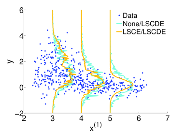
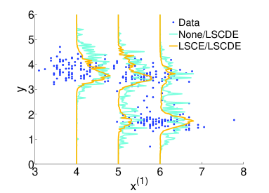
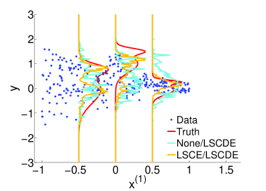
First, we illustrate the behavior of the plain LSCDE (None/LSCDE) and the proposed method (LSCE/LSCDE). The datasets illustrated in Figure 2 have $d_{\textbf{x}}=5$, $d_{\textbf{y}}=1$, and $d_{\textbf{z}}=1$. The first dimension of input $\boldsymbol{x}$ and output $y$ of the samples are plotted in the graphs, and other 4 dimensions of $\boldsymbol{x}$ are just standard normal noise. The results show that the plain LSCDE does not perform well due to the irrelevant noise dimensions of $\boldsymbol{x}$, while the proposed method gives much better estimates.

(a) Illustrative data

(b) Bone mineral density

(c) Old faithful geyser

Figure 2: Examples of conditional density estimation by plain LSCDE (None/LSCDE) and the proposed method (LSCE/LSCDE).

3.2 Artificial Datasets

For $d_{\textbf{x}}=5$, $d_{\textbf{y}}=1$, $\boldsymbol{x}\sim\mathcal{N}(\boldsymbol{x}|\boldsymbol{0},\boldsymbol{I}_{5})$, and $\epsilon\sim\mathcal{N}(\epsilon|0,0.25^{2})$, where $\mathcal{N}(\cdot|\boldsymbol{\mu},\boldsymbol{\Sigma})$ denotes the normal distribution with mean $\boldsymbol{\mu}$ and covariance matrix $\boldsymbol{\Sigma}$, we consider the following artificial datasets:

(a)

$d_{\textbf{z}}=2$ and $y=(x^{(1)})^{2}+(x^{(2)})^{2}+\epsilon$.

(b)

$d_{\textbf{z}}=1$ and $y=x^{(2)}+(x^{(2)})^{2}+(x^{(2)})^{3}+\epsilon$.

(a) Artificial data 1

(b) Artificial data 2

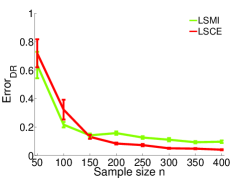
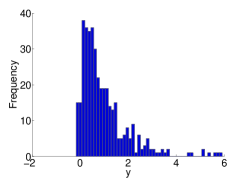
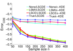
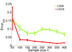
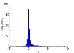
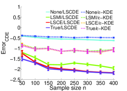
Figure 3: Left column: The mean and standard error of the dimensionality reduction error over 20 runs on the artificial datasets. Middle column: Histograms of $\{y_{i}\}_{i=1}^{400}$. Right column: The mean and standard error of the conditional density estimation error over 20 runs.

The left column of Figure 3 shows the dimensionality reduction error between true $\boldsymbol{W}^{*}$ and its estimate $\widehat{\boldsymbol{W}}$ for different sample size $n$, measured by

$$\mathrm{Error}_{\mathrm{DR}}=\|\widehat{\boldsymbol{W}}^{\top}\widehat{\boldsymbol{W}}-{\boldsymbol{W}^{*}}^{\top}\boldsymbol{W}^{*}\|_{\mathrm{Frobenius}},$$

where $\|\cdot\|_{\mathrm{Frobenius}}$ denotes the Frobenius norm. LSMI and LSCE perform similarly for the dataset (a), while LSCE clearly outperforms LSMI for the datasets (b). To explain this difference, we plot the histograms of $\{y\}_{i=1}^{400}$ in the middle column of Figure 3. They show that the profile of the histogram (which is a sample approximation of $p(y)$) in the dataset (b) is much sharper than that in the dataset (a). As discussed in Section 2.8, the density ratio $\frac{p(\boldsymbol{z},\boldsymbol{y})}{p(\boldsymbol{z})p(\boldsymbol{y})}$ used in LSMI contains $p(\boldsymbol{y})$. Thus, for the dataset (b), the density ratio $\frac{p(\boldsymbol{z},\boldsymbol{y})}{p(\boldsymbol{z})p(\boldsymbol{y})}$ would be highly non-smooth and thus is hard to approximate. On the other hand, the density ratio used in SCE is $\frac{p(\boldsymbol{z},\boldsymbol{y})}{p(\boldsymbol{z})}$, where $p(\boldsymbol{y})$ is not included. Therefore, $\frac{p(\boldsymbol{z},\boldsymbol{y})}{p(\boldsymbol{z})}$ would be smoother than $\frac{p(\boldsymbol{z},\boldsymbol{y})}{p(\boldsymbol{z})p(\boldsymbol{y})}$ and $\frac{p(\boldsymbol{z},\boldsymbol{y})}{p(\boldsymbol{z})}$ is easier to estimate than $\frac{p(\boldsymbol{z},\boldsymbol{y})}{p(\boldsymbol{z})p(\boldsymbol{y})}$.

The right column of Figure 3 plots the conditional density estimation error between true $p(\boldsymbol{y}|\boldsymbol{x})$ and its estimate $\widehat{p}(\boldsymbol{y}|\boldsymbol{x})$, evaluated by the squared-loss:

$$\mathrm{Error}_{\mathrm{CDE}}=\frac{1}{2n^{\prime}}\sum_{i=1}^{n^{\prime}}\int\widehat{p}(\boldsymbol{y}|\widetilde{\boldsymbol{x}}_{i})^{2}\mathrm{d}\boldsymbol{y}-\frac{1}{n^{\prime}}\sum_{i=1}^{n^{\prime}}\widehat{p}(\widetilde{\boldsymbol{y}}_{i}|\widetilde{\boldsymbol{x}}_{i}),$$

where $\{(\widetilde{\boldsymbol{x}}_{i},\widetilde{\boldsymbol{y}}_{i})\}_{i=1}^{n^{\prime}}$ is a set of test samples that have not been used for training. We set $n^{\prime}=1000$. The graphs show that LSCDE overall outperforms $\epsilon$-KDE for both datasets. For the dataset (a), LSMI/LSCDE and LSCE/LSCDE perform equally well, which are much better than no dimension reduction (None/LSCDE) and are comparable to the method with the true subspace (True/LSCDE). For the dataset (b), LSCE/LSCDE outperforms LSMI/LSCDE and None/LSCDE, and is comparable to the method with the true subspace (True/LSCDE).

3.3 Benchmark Datasets

Next, we use the UCI benchmark datasets (Bache and Lichman, 2013). We randomly select $n$ samples from each dataset for training, and the rest are used to measure the conditional density estimation error in the test phase. Since the dimensionality of the subspace $d_{\textbf{z}}$ is unknown, we chose it by cross-validation. The results are summarized in Table 1, showing that that the proposed method, LSCE/LSCDE works well overall. Table 2 describes the dimensionalities selected by cross-validation, showing that both LSCE and LSMI reduce the dimensionalty significantly. For “Housing”, “AutoMPG”, “Energy”, and “Stock”, LSMI/LSCDE tends to more aggressively reduce the dimensionality than LSCE/LSCDE.

Table 1: Mean and standard error of the conditional density estimation error over 10 runs. The best method in term of the mean error and comparable methods according to the two-sample paired t-test at the significance level $5\%$ are specified by bold face.

Dataset	$(d_{\textbf{x}},d_{\textbf{y}})$	$n$	LSCE		LSMI		No reduction		Scale
			LSCDE	$\epsilon$-KDE	LSCDE	$\epsilon$-KDE	LSCDE	$\epsilon$-KDE
Housing	$(13,1)$	100	$\boldsymbol{-1.73(0.09)}$	$-1.57(0.11)$	$\boldsymbol{-1.91(0.05)}$	$-1.62(0.08)$	$-1.41(0.05)$	$-1.13(0.01)$	$\times 1$
Auto MPG	$(7,1)$	100	$\boldsymbol{-1.80(0.04)}$	$\boldsymbol{-1.74(0.06)}$	$\boldsymbol{-1.85(0.04)}$	$\boldsymbol{-1.77(0.05)}$	$\boldsymbol{-1.75(0.04)}$	$-1.46(0.04)$	$\times 1$
Servo	$(4,1)$	50	$\boldsymbol{-2.92(0.18)}$	$\boldsymbol{-3.03(0.14)}$	$\boldsymbol{-2.69(0.18)}$	$\boldsymbol{-2.95(0.11)}$	$-2.62(0.09)$	$-2.72(0.06)$	$\times 1$
Yacht	$(6,1)$	80	$\boldsymbol{-6.46(0.02)}$	$\boldsymbol{-6.23(0.14)}$	$-5.63(0.26)$	$-5.47(0.29)$	$-1.72(0.04)$	$-2.95(0.02)$	$\times 1$
Physicochem	$(9,1)$	500	$\boldsymbol{-1.19(0.01)}$	$-0.99(0.02)$	$\boldsymbol{-1.20(0.01)}$	$-0.97(0.02)$	$\boldsymbol{-1.19(0.01)}$	$-0.91(0.01)$	$\times 1$
White Wine	$(11,1)$	400	$-2.31(0.01)$	$\boldsymbol{-2.47(0.15)}$	$\boldsymbol{-2.35(0.02)}$	$\boldsymbol{-2.60(0.12)}$	$-2.06(0.01)$	$-1.89(0.01)$	$\times 1$
Red Wine	$(11,1)$	300	$\boldsymbol{-2.85(0.02)}$	$-1.95(0.17)$	$\boldsymbol{-2.82(0.03)}$	$-1.93(0.17)$	$-2.03(0.02)$	$-1.13(0.04)$	$\times 1$
Forest Fires	$(12,1)$	100	$\boldsymbol{-7.18(0.02)}$	$-6.93(0.03)$	$-6.93(0.04)$	$-6.93(0.02)$	$-3.40(0.07)$	$-6.96(0.02)$	$\times 1$
Concrete	$(8,1)$	300	$\boldsymbol{-1.36(0.03)}$	$-1.20(0.06)$	$\boldsymbol{-1.30(0.03)}$	$-1.18(0.04)$	$-1.11(0.02)$	$-0.80(0.03)$	$\times 1$
Energy	$(8,2)$	200	$\boldsymbol{-7.13(0.04)}$	$-4.18(0.22)$	$-6.04(0.47)$	$-3.41(0.49)$	$-2.12(0.06)$	$-1.95(0.14)$	$\times 10$
Stock	$(7,2)$	100	$-8.37(0.53)$	$\boldsymbol{-9.75(0.37)}$	$\boldsymbol{-9.42(0.50)}$	$\boldsymbol{-10.27(0.33)}$	$-7.35(0.13)$	$-9.25(0.14)$	$\times 1$
2 Joints	$(6,4)$	100	$\boldsymbol{-10.49(0.86)}$	$-7.50(0.54)$	$\boldsymbol{-8.00(0.84)}$	$-7.44(0.60)$	$-3.95(0.13)$	$-3.65(0.14)$	$\times 1$
4 Joints	$(12,8)$	200	$\boldsymbol{-2.81(0.21)}$	$-1.73(0.14)$	$-2.06(0.25)$	$-1.38(0.16)$	$-0.83(0.03)$	$-0.75(0.01)$	$\times 10$
9 Joints	$(27,18)$	500	$\boldsymbol{-8.37(0.83)}$	$-2.44(0.17)$	$\boldsymbol{-9.74(0.63)}$	$-2.37(0.51)$	$-1.60(0.36)$	$-0.89(0.02)$	$\times 100$
Sumi-e 1	$(9,6)$	200	$\boldsymbol{-9.96(1.60)}$	$-1.49(0.78)$	$\boldsymbol{-6.00(1.28)}$	$1.24(1.99)$	$-5.98(0.80)$	$-0.17(0.44)$	$\times 10$
Sumi-e 2	$(9,6)$	250	$\boldsymbol{-16.83(1.70)}$	$-2.22(0.97)$	$-9.54(1.31)$	$-3.12(0.75)$	$-7.69(0.62)$	$-0.66(0.13)$	$\times 10$
Sumi-e 3	$(9,6)$	300	$\boldsymbol{-24.92(1.92)}$	$-6.61(1.25)$	$-18.0(2.61)$	$-4.47(0.68)$	$-8.98(0.66)$	$-1.45(0.43)$	$\times 10$

Table 2: Mean and standard error of the chosen dimensionality over 10 runs.

Data set	$(d_{\textbf{x}},d_{\textbf{y}})$	LSCE		LSMI
		LSCDE	$\epsilon$-KDE	LSCDE	$\epsilon$-KDE
Housing	$(13,1)$	$3.9(0.74)$	$2.0(0.79)$	$2.0(0.39)$	$1.3(0.15)$
Auto MPG	$(7,1)$	$3.2(0.66)$	$1.3(0.15)$	$2.1(0.67)$	$1.1(0.10)$
Servo	$(4,1)$	$1.9(0.35)$	$2.4(0.40)$	$2.2(0.33)$	$1.6(0.31)$
Yacht	$(6,1)$	$1.0(0.00)$	$1.0(0.00)$	$1.0(0.00)$	$1.0(0.00)$
Physicochem	$(9,1)$	$6.5(0.58)$	$1.9(0.28)$	$6.6(0.58)$	$2.6(0.86)$
White Wine	$(11,1)$	$1.2(0.13)$	$1.0(0.00)$	$1.4(0.31)$	$1.0(0.00)$
Red Wine	$(11,1)$	$1.0(0.00)$	$1.3(0.15)$	$1.2(0.20)$	$1.0(0.00)$
Forest Fires	$(12,1)$	$1.2(0.20)$	$4.9(0.99)$	$1.4(0.22)$	$6.8(1.23)$
Concrete	$(8,1)$	$1.0(0.00)$	$1.0(0.00)$	$1.2(0.13)$	$1.0(0.00)$
Energy	$(8,2)$	$5.9(0.10)$	$3.9(0.80)$	$2.1(0.10)$	$2.0(0.30)$
Stock	$(7,2)$	$3.2(0.83)$	$2.1(0.59)$	$2.1(0.60)$	$2.7(0.67)$
2 Joints	$(6,4)$	$2.9(0.31)$	$2.7(0.21)$	$2.5(0.31)$	$2.0(0.00)$
4 Joints	$(12,8)$	$5.2(0.68)$	$6.2(0.63)$	$5.4(0.67)$	$4.6(0.43)$
9 Joints	$(27,18)$	$13.8(1.28)$	$15.3(0.94)$	$11.4(0.75)$	$13.2(1.02)$
Sumi-e 1	$(9,6)$	$5.3(0.72)$	$2.9(0.85)$	$4.5(0.45)$	$3.2(0.76)$
Sumi-e 2	$(9,6)$	$4.2(0.55)$	$4.4(0.85)$	$4.6(0.87)$	$2.5(0.78)$
Sumi-e 3	$(9,6)$	$3.6(0.50)$	$2.7(0.76)$	$2.6(0.40)$	$1.6(0.27)$

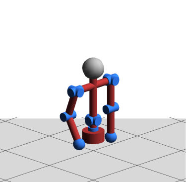
Figure 4: Simulator of the upper-body part of the humanoid robot CB-i.

3.4 Humanoid Robot

We evaluate the performance of the proposed method on humanoid robot transition estimation. We use a simulator of the upper-body part of the humanoid robot CB-i (Cheng et al., 2007) (see Figure 4). The robot has 9 controllable joints: shoulder pitch, shoulder roll, elbow pitch of the right arm, shoulder pitch, shoulder roll, elbow pitch of the left arm, waist yaw, torso roll, and torso pitch joints.

Posture of the robot is described by 18-dimensional real-valued state vector $\boldsymbol{s}$, which corresponds to the angle and angular velocity of each joint in radians and radians per seconds, respectively. We can control the robot by sending the action command $\boldsymbol{a}$ to the system. The action command $\boldsymbol{a}$ is a 9-dimensional real-valued vector, which corresponds to the target angle of each joint. When the robot is currently at state $\boldsymbol{s}$ and receives action $\boldsymbol{a}$, the physical control system of the simulator calculates the amount of torques to be applied to each joint. These torques are calculated by the proportional-derivative (PD) controller as

$$\tau_{i}=K_{p_{i}}(a_{i}-s_{i})-K_{d_{i}}\dot{s}_{i},$$

where $s_{i}$, $\dot{s}_{i}$, and $a_{i}$ denote the current angle, the current angular velocity, and the received target angle of the $i$-th joint, respectively. $K_{p_{i}}$ and $K_{d_{i}}$ denote the position and velocity gains for the $i$-th joint, respectively. We set $K_{p_{i}}=2000$ and $K_{d_{i}}=100$ for all joints except that $K_{p_{i}}=200$ and $K_{d_{i}}=10$ for the elbow pitch joints. After the torques are applied to the joints, the physical control system update the state of the robot to $\boldsymbol{s}^{\prime}$.

In the experiment, we randomly choose the action vector $\boldsymbol{a}$ and simulate a noisy control system by adding a bimodal Gaussian noise vector. More specifically, the action $a_{i}$ of the $i$-th joint is first drawn from uniform distribution on $[s_{i}-0.087,s_{i}+0.087]$. The drawn action is then contaminated by Gaussian noise with mean 0 and standard deviation 0.034 with probability 0.6 and Gaussian noise with mean -0.087 and standard deviation 0.034 with probability 0.4. By repeatedly control the robot $n$ times, we obtain the transition samples $\{(\boldsymbol{s}_{j},\boldsymbol{a}_{j},\boldsymbol{s}^{\prime}_{j})\}_{j=1}^{n}$. Our goal is to learn the system dynamic as a state transition probability $p(\boldsymbol{s}^{\prime}|\boldsymbol{s},\boldsymbol{a})$ from these samples. Thus, as the conditional density estimation problem, the state-action pair $(\boldsymbol{s}^{\top},\boldsymbol{a}^{\top})^{\top}$ is regarded as input variable $\boldsymbol{x}$, while the next state $\boldsymbol{s}^{\prime}$ is regarded as output variable $\boldsymbol{y}$. Such state-transition probabilities are highly useful in model-based reinforcement learning (Sutton and Barto, 1998).

We consider three scenarios: Using only 2 joints (right shoulder pitch and right elbow pitch), only 4 joints (in addition, right shoulder roll and waist yaw), and all 9 joints. Thus, $d_{\textbf{x}}=6$ and $d_{\textbf{y}}=4$ for the 2-joint case, $d_{\textbf{x}}=12$ and $d_{\textbf{y}}=8$ for the 4-joint case, and $d_{\textbf{x}}=27$ and $d_{\textbf{y}}=18$ for the 9-joint case. We generate $500$, $1000$, and $1500$ transition samples for the 2-joint, 4-joint, and 9-joint cases. We then randomly choose $n=100$, $200$, and $500$ samples for training, and use the rest for evaluating the test error. The results are summarized also in Table 1, showing that the proposed method performs well for the all three cases. Table 2 describes the dimensionalities selected by cross-validation, showing that the humanoid robot’s transition is highly redundant.

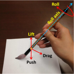
Figure 5: Three actions of the brush, which is modeled as the footprint on a paper canvas.

3.5 Computer Art

Finally, we consider the transition estimation problem in sumi-e style brush drawings for non-photorealistic rendering (Xie et al., 2012). Our aim is to learn the brush dynamics as state transition probability $p(\boldsymbol{s^{\prime}}|\boldsymbol{s},\boldsymbol{a})$ from the real artists’ stroke-drawing samples.

From a video of real brush stroks, we extract footprints and identify corresponding 3-dimensional actions (see Figure 5). The state vector consists of six measurements: the angle of the velocity vector and the heading direction of the footprint relative to the medial axis of the drawing shape, the ratio of the offset distance from the center of the footprint to the nearest point on the medial axis over the radius of the footprint, the relative curvatures of the nearest current point and the next point on the medial axis, and the binary signal of the reverse driving or not. Thus, the state transition probability $p(\boldsymbol{s^{\prime}}|\boldsymbol{s},\boldsymbol{a})$ has $9$-dimensional input and $6$-dimensional output. We collect $722$ transition samples in total. We randomly choose $n=200,250$, and $300$ for training and use the rest for testing.

The estimation results summarized at the bottom of Table 1 and Table 2. These tables show that there exists a low-dimensional sufficient subspace and the proposed method can successfully find it.

4 Conclusion

We proposed a new method for conditional density estimation in high-dimension problems. The key idea of the proposed method is to perform sufficient dimensionality reduction by minimizing the square-loss conditional entropy (SCE), which can be estimated by least-squares conditional density estimation. Thus, dimensionality reduction and conditional density estimation are carried out simultaneously in an integrated manner. We have also shown that SCE and the squared-loss mutual information (SMI) are similar but different in that the output density is included in the denominator of the density ratio in SMI. This means that estimation of SMI is hard when the output density is fluctuated, while the proposed method using SCE does not suffer from this problem. The effectiveness of the proposed method was demonstrated through extensive experiments including humanoid robot transition and computer art.

Appendix A Proof of Theorem 1

The $\widetilde{\mathrm{SCE}}$ is defined as

$$\widetilde{\mathrm{SCE}}(\boldsymbol{Y}|\boldsymbol{Z}) =-\frac{1}{2}\iint p(\boldsymbol{y}|\boldsymbol{z})^{2}p(\boldsymbol{z})\mathrm{d}\boldsymbol{z}\mathrm{d}\boldsymbol{y}.$$

Then we have

$$\widetilde{\mathrm{SCE}}(\boldsymbol{Y}|\boldsymbol{Z})-\widetilde{\mathrm{SCE}}(\boldsymbol{Y}|\boldsymbol{X}) =\frac{1}{2}\iint p(\boldsymbol{y}|\boldsymbol{x})^{2}p(\boldsymbol{x})\mathrm{d}\boldsymbol{y}\mathrm{d}\boldsymbol{x}-\frac{1}{2}\iint p(\boldsymbol{y}|\boldsymbol{z})^{2}p(\boldsymbol{z})\mathrm{d}\boldsymbol{z}\mathrm{d}\boldsymbol{y}$$

$$=\frac{1}{2}\iint p(\boldsymbol{y}|\boldsymbol{x})^{2}p(\boldsymbol{x})\mathrm{d}\boldsymbol{x}\mathrm{d}\boldsymbol{y}+\frac{1}{2}\iint p(\boldsymbol{y}|\boldsymbol{z})^{2}p(\boldsymbol{z})\mathrm{d}\boldsymbol{z}\mathrm{d}\boldsymbol{y}$$

$$\ \ \ -\iint p(\boldsymbol{y}|\boldsymbol{z})^{2}p(\boldsymbol{z})\mathrm{d}\boldsymbol{z}\mathrm{d}\boldsymbol{y}.$$

Let $p(\boldsymbol{x})=p(\boldsymbol{z},\boldsymbol{z}_{\perp})$, and $\mathrm{d}\boldsymbol{x}=\mathrm{d}\boldsymbol{z}\mathrm{d}\boldsymbol{z}_{\perp}$. Then the final term can be expressed as

$$\iint p(\boldsymbol{y}|\boldsymbol{z})^{2}p(\boldsymbol{z})\mathrm{d}\boldsymbol{z}\mathrm{d}\boldsymbol{y} =\iint\frac{p(\boldsymbol{z},\boldsymbol{y})}{p(\boldsymbol{z})}\frac{p(\boldsymbol{z},\boldsymbol{y})}{p(\boldsymbol{z})}p(\boldsymbol{z})\mathrm{d}\boldsymbol{z}\mathrm{d}\boldsymbol{y}$$

$$=\iint\frac{p(\boldsymbol{z},\boldsymbol{y})}{p(\boldsymbol{z})}p(\boldsymbol{z},\boldsymbol{y})\mathrm{d}\boldsymbol{z}\mathrm{d}\boldsymbol{y}$$

$$=\iint\frac{p(\boldsymbol{z},\boldsymbol{y})}{p(\boldsymbol{z})}p(\boldsymbol{z}_{\perp}|\boldsymbol{z},\boldsymbol{y})p(\boldsymbol{z},\boldsymbol{y})\mathrm{d}\boldsymbol{z}\mathrm{d}\boldsymbol{z}_{\perp}\mathrm{d}\boldsymbol{y}$$

$$=\iint\frac{p(\boldsymbol{z},\boldsymbol{y})}{p(\boldsymbol{z})}p(\boldsymbol{z},\boldsymbol{z}_{\perp},\boldsymbol{y})\mathrm{d}\boldsymbol{z}\mathrm{d}\boldsymbol{z}_{\perp}\mathrm{d}\boldsymbol{y}$$

$$=\iint\frac{p(\boldsymbol{z},\boldsymbol{y})}{p(\boldsymbol{z})}p(\boldsymbol{x},\boldsymbol{y})\mathrm{d}\boldsymbol{x}\mathrm{d}\boldsymbol{y}$$

$$=\iint\frac{p(\boldsymbol{z},\boldsymbol{y})}{p(\boldsymbol{z})}\frac{p(\boldsymbol{x},\boldsymbol{y})}{p(\boldsymbol{x})}p(\boldsymbol{x})\mathrm{d}\boldsymbol{x}\mathrm{d}\boldsymbol{y}$$

$$=\iint p(\boldsymbol{y}|\boldsymbol{z})p(\boldsymbol{y}|\boldsymbol{x})p(\boldsymbol{x})\mathrm{d}\boldsymbol{x}\mathrm{d}\boldsymbol{y},$$

where $p(\boldsymbol{z},\boldsymbol{z}_{\perp},\boldsymbol{y})=p(\boldsymbol{x},\boldsymbol{y})$, and $\mathrm{d}\boldsymbol{z}\mathrm{d}\boldsymbol{z}_{\perp}=\mathrm{d}\boldsymbol{x}$ are used. Therefore,

$$\widetilde{\mathrm{SCE}}(\boldsymbol{Y}|\boldsymbol{Z})-\widetilde{\mathrm{SCE}}(Y|X) =\frac{1}{2}\iint p(\boldsymbol{y}|\boldsymbol{x})^{2}p(\boldsymbol{x})\mathrm{d}\boldsymbol{x}\mathrm{d}\boldsymbol{y}+\frac{1}{2}\iint p(\boldsymbol{y}|\boldsymbol{z})^{2}p(\boldsymbol{z})\mathrm{d}\boldsymbol{z}\mathrm{d}\boldsymbol{y}$$

$$\ \ \ -\iint p(\boldsymbol{y}|\boldsymbol{z})p(\boldsymbol{y}|\boldsymbol{x})p(\boldsymbol{x})\mathrm{d}\boldsymbol{x}\mathrm{d}\boldsymbol{y}$$

$$=\frac{1}{2}\iint\left(p(\boldsymbol{y}|\boldsymbol{x})-p(\boldsymbol{y}|\boldsymbol{z})\right)^{2}p(\boldsymbol{x})\mathrm{d}\boldsymbol{x}\mathrm{d}\boldsymbol{y}$$

We can also express $p(\boldsymbol{y}|\boldsymbol{x})$ in term of $p(\boldsymbol{y}|\boldsymbol{z})$ as

$$p(\boldsymbol{y}|\boldsymbol{x}) =\frac{p(\boldsymbol{x},\boldsymbol{y})}{p(\boldsymbol{x})}$$

$$=\frac{p(\boldsymbol{x},\boldsymbol{y})}{p(\boldsymbol{x})}\frac{p(\boldsymbol{z},\boldsymbol{y})}{p(\boldsymbol{z},\boldsymbol{y})}$$

$$=\frac{p(\boldsymbol{x},\boldsymbol{y})p(\boldsymbol{z},\boldsymbol{y})}{p(\boldsymbol{z}_{\perp}|\boldsymbol{z})p(\boldsymbol{z})p(\boldsymbol{y}|\boldsymbol{z})p(\boldsymbol{z})}$$

$$=\frac{p(\boldsymbol{z},\boldsymbol{z}_{\perp},\boldsymbol{y})p(\boldsymbol{z},\boldsymbol{y})}{p(\boldsymbol{z}_{\perp}|\boldsymbol{z})p(\boldsymbol{z})p(\boldsymbol{y}|\boldsymbol{z})p(\boldsymbol{z})}$$

$$=\frac{p(\boldsymbol{z}_{\perp},\boldsymbol{y}|\boldsymbol{z})p(\boldsymbol{z},\boldsymbol{y})}{p(\boldsymbol{z}_{\perp}|\boldsymbol{z})p(\boldsymbol{y}|\boldsymbol{z})p(\boldsymbol{z})}$$

$$=\frac{p(\boldsymbol{z}_{\perp},\boldsymbol{y}|\boldsymbol{z})}{p(\boldsymbol{z}_{\perp}|\boldsymbol{z})p(\boldsymbol{y}|\boldsymbol{z})}p(\boldsymbol{y}|\boldsymbol{z})$$

Finally, we obtain

$$\widetilde{\mathrm{SCE}}(\boldsymbol{Y}|\boldsymbol{Z})-\widetilde{\mathrm{SCE}}(\boldsymbol{Y}|\boldsymbol{X}) =\frac{1}{2}\iint\left(p(\boldsymbol{y}|\boldsymbol{x})-p(\boldsymbol{y}|\boldsymbol{z})\right)^{2}p(\boldsymbol{x})\mathrm{d}\boldsymbol{x}\mathrm{d}\boldsymbol{y}$$

$$=\frac{1}{2}\iint\left(\frac{p(\boldsymbol{z}_{\perp},\boldsymbol{y}|\boldsymbol{z})}{p(\boldsymbol{z}_{\perp}|\boldsymbol{z})p(\boldsymbol{y}|\boldsymbol{z})}p(\boldsymbol{y}|\boldsymbol{z})-p(\boldsymbol{y}|\boldsymbol{z})\right)^{2}p(\boldsymbol{x})\mathrm{d}\boldsymbol{x}\mathrm{d}\boldsymbol{y}$$

$$=\frac{1}{2}\iint\left(\frac{p(\boldsymbol{z}_{\perp},\boldsymbol{y}|\boldsymbol{z})}{p(\boldsymbol{z}_{\perp}|\boldsymbol{z})p(\boldsymbol{y}|\boldsymbol{z})}-1\right)^{2}p(\boldsymbol{y}|\boldsymbol{z})^{2}p(\boldsymbol{x})\mathrm{d}\boldsymbol{x}\mathrm{d}\boldsymbol{y}$$

$$\geq 0,$$

which concludes the proof.

Appendix B Derivatives of SCE

Here we show the formula of derivatives of $\widehat{\mathrm{SCE}}(Y|Z)$ using LSCE estimator. SCE approximation by LSCE estimator is

$$\widehat{\mathrm{SCE}}(\boldsymbol{Y}|\boldsymbol{Z}) =\frac{1}{2}\widehat{\boldsymbol{\alpha}}^{\top}\widehat{\boldsymbol{G}}\widehat{\boldsymbol{\alpha}}-\widehat{\boldsymbol{h}}^{\top}\widehat{\boldsymbol{\alpha}}.$$

Taking its partial derivatives with respect to $\boldsymbol{W}$ and we obtain

$$\frac{\partial\widehat{\mathrm{SCE}}}{\partial W_{l,l^{\prime}}} =-\frac{1}{2}\frac{\partial\widehat{\boldsymbol{\alpha}}^{\top}\widehat{\boldsymbol{G}}\widehat{\boldsymbol{\alpha}}}{\partial W_{l,l^{\prime}}}-\frac{\partial\widehat{\boldsymbol{h}}^{\top}\widehat{\boldsymbol{\alpha}}}{\partial W_{l,l^{\prime}}}$$

$$=\frac{1}{2}\left(\frac{\partial\widehat{\boldsymbol{\alpha}}^{\top}}{\partial W_{l,l^{\prime}}}\widehat{\boldsymbol{G}}\widehat{\boldsymbol{\alpha}}+\frac{(\widehat{\boldsymbol{G}}\widehat{\boldsymbol{\alpha}})^{\top}}{\partial W_{l,l^{\prime}}}\widehat{\boldsymbol{\alpha}}\right)-\frac{\partial\widehat{\boldsymbol{\alpha}}^{\top}}{\partial W_{l,l^{\prime}}}\widehat{\boldsymbol{h}}-\frac{\partial\widehat{\boldsymbol{h}}^{\top}}{\partial W_{l,l^{\prime}}}\widehat{\boldsymbol{\alpha}}$$

$$=\frac{1}{2}\frac{\partial\widehat{\boldsymbol{\alpha}}^{\top}}{\partial W_{l,l^{\prime}}}\widehat{\boldsymbol{G}}\widehat{\boldsymbol{\alpha}}+\frac{1}{2}\frac{\partial\widehat{\boldsymbol{\alpha}}^{\top}}{\partial W_{l,l^{\prime}}}\widehat{\boldsymbol{G}}\widehat{\boldsymbol{\alpha}}+\frac{1}{2}\widehat{\boldsymbol{\alpha}}^{\top}\frac{\partial\widehat{\boldsymbol{G}}}{\partial W_{l,l^{\prime}}}\widehat{\boldsymbol{\alpha}}-\frac{\partial\widehat{\boldsymbol{\alpha}}^{\top}}{\partial W_{l,l^{\prime}}}\widehat{\boldsymbol{h}}-\frac{\partial\widehat{\boldsymbol{h}}^{\top}}{\partial W_{l,l^{\prime}}}\widehat{\boldsymbol{\alpha}}$$

$$=\frac{\partial\widehat{\boldsymbol{\alpha}}^{\top}}{\partial W_{l,l^{\prime}}}\widehat{\boldsymbol{G}}\widehat{\boldsymbol{\alpha}}+\frac{1}{2}\widehat{\boldsymbol{\alpha}}^{\top}\frac{\partial\widehat{\boldsymbol{G}}}{\partial W_{l,l^{\prime}}}\widehat{\boldsymbol{\alpha}}-\frac{\partial\widehat{\boldsymbol{\alpha}}^{\top}}{\partial W_{l,l^{\prime}}}\widehat{\boldsymbol{h}}-\frac{\partial\widehat{\boldsymbol{h}}^{\top}}{\partial W_{l,l^{\prime}}}\widehat{\boldsymbol{\alpha}}.$$ (12)

Next we consider the partial derivatives of $\widehat{\boldsymbol{\alpha}}$ as follows

$$\frac{\partial\widehat{\boldsymbol{\alpha}}}{\partial W_{l,l^{\prime}}} =\frac{\partial(\widehat{\boldsymbol{G}}+\lambda\boldsymbol{I})^{-1}\widehat{\boldsymbol{h}}}{\partial W_{l,l^{\prime}}}$$

$$=\frac{\partial(\widehat{\boldsymbol{G}}+\lambda\boldsymbol{I})^{-1}}{\partial W_{l,l^{\prime}}}\widehat{\boldsymbol{h}}+(\widehat{\boldsymbol{G}}+\lambda\boldsymbol{I})^{-1}\frac{\partial\widehat{\boldsymbol{h}}}{\partial W_{l,l^{\prime}}}$$

$$\frac{\partial\widehat{\boldsymbol{\alpha}}^{\top}}{\partial W_{l,l^{\prime}}} =(\frac{\partial(\widehat{\boldsymbol{G}}+\lambda\boldsymbol{I})^{-1}}{\partial W_{l,l^{\prime}}}\widehat{\boldsymbol{h}})^{\top}+\frac{\partial\widehat{\boldsymbol{h}}^{\top}}{\partial W_{l,l^{\prime}}}(\widehat{\boldsymbol{G}}+\lambda\boldsymbol{I})^{-1}.$$ (13)

Using $\frac{\partial\boldsymbol{X}^{-1}}{\partial t}=-\boldsymbol{X}^{-1}\frac{\partial\boldsymbol{X}}{\partial t}\boldsymbol{X}^{-1}$, we obtain

$$\frac{\partial(\widehat{\boldsymbol{G}}+\lambda\boldsymbol{I})^{-1}}{\partial W_{l,l^{\prime}}}\widehat{\boldsymbol{h}} =-(\widehat{\boldsymbol{G}}+\lambda\boldsymbol{I})^{-1}\frac{\partial\widehat{\boldsymbol{G}}}{\partial W_{l,l^{\prime}}}(\widehat{\boldsymbol{G}}+\lambda\boldsymbol{I})^{-1}\widehat{\boldsymbol{h}}-(\widehat{\boldsymbol{G}}+\lambda\boldsymbol{I})^{-1}\frac{\partial\lambda\boldsymbol{I}}{\partial W_{l,l^{\prime}}}(\widehat{\boldsymbol{G}}+\lambda\boldsymbol{I})^{-1}\widehat{\boldsymbol{h}}$$

$$=-(\widehat{\boldsymbol{G}}+\lambda\boldsymbol{I})^{-1}\frac{\partial\widehat{\boldsymbol{G}}}{\partial W_{l,l^{\prime}}}\widehat{\boldsymbol{\alpha}}-0$$

$$(\frac{\partial(\widehat{\boldsymbol{G}}+\lambda\boldsymbol{I})^{-1}}{\partial W_{l,l^{\prime}}}\widehat{\boldsymbol{h}})^{\top} =-\widehat{\boldsymbol{\alpha}}^{\top}\frac{\partial\widehat{\boldsymbol{G}}}{\partial W_{l,l^{\prime}}}(\widehat{\boldsymbol{G}}+\lambda\boldsymbol{I})^{-1}.$$ (14)

Substitute Eq.(14) into Eq.(13) to obtain

$$\frac{\partial\widehat{\boldsymbol{\alpha}}^{\top}}{\partial W_{l,l^{\prime}}} =-\widehat{\boldsymbol{\alpha}}^{\top}\frac{\partial\widehat{\boldsymbol{G}}}{\partial W_{l,l^{\prime}}}(\widehat{\boldsymbol{G}}+\lambda\boldsymbol{I})^{-1}+\frac{\partial\widehat{\boldsymbol{h}}^{\top}}{\partial W_{l,l^{\prime}}}(\widehat{\boldsymbol{G}}+\lambda\boldsymbol{I})^{-1}.$$ (15)

Finally, by substitute Eq.(15) into Eq.(12) and use $(\widehat{\boldsymbol{G}}+\lambda\boldsymbol{I})^{-1}\widehat{\boldsymbol{G}}\widehat{\boldsymbol{\alpha}}=\widehat{\boldsymbol{\beta}}$, we have

$$\frac{\partial\widehat{\mathrm{SCE}}}{\partial W_{l,l^{\prime}}} =-\widehat{\boldsymbol{\alpha}}^{\top}\frac{\partial\widehat{\boldsymbol{G}}}{\partial W_{l,l^{\prime}}}\widehat{\boldsymbol{\beta}}+\frac{\partial\widehat{\boldsymbol{h}}^{\top}}{\partial W_{l,l^{\prime}}}\widehat{\boldsymbol{\beta}}+\frac{1}{2}\widehat{\boldsymbol{\alpha}}^{\top}\frac{\partial\widehat{\boldsymbol{G}}}{\partial W_{l,l^{\prime}}}\widehat{\boldsymbol{\alpha}}$$

$$\ \ \ \ +\widehat{\boldsymbol{\alpha}}^{\top}\frac{\partial\widehat{\boldsymbol{G}}}{\partial W_{l,l^{\prime}}}\widehat{\boldsymbol{\alpha}}-\frac{\partial\widehat{\boldsymbol{h}}^{\top}}{\partial W_{l,l^{\prime}}}\widehat{\boldsymbol{\alpha}}-\frac{\partial\widehat{\boldsymbol{h}}^{\top}}{\partial W_{l,l^{\prime}}}\widehat{\boldsymbol{\alpha}}$$

$$=\widehat{\boldsymbol{\alpha}}^{\top}\frac{\partial\widehat{\boldsymbol{G}}}{\partial W_{l,l^{\prime}}}(\frac{3}{2}\widehat{\boldsymbol{\alpha}}-\widehat{\boldsymbol{\beta}})+\frac{\partial\widehat{\boldsymbol{h}}^{\top}}{\partial W_{l,l^{\prime}}}(\widehat{\boldsymbol{\beta}}-2\widehat{\boldsymbol{\alpha}}),$$

where the partial derivatives of $\widehat{\boldsymbol{G}}$ and $\widehat{\boldsymbol{h}}$ depend on the choice of basis function.

Here we consider the Gaussian basis function described in Section 2.4. Their partial derivatives are given by

$$\frac{\partial\widehat{G}_{k,k^{\prime}}}{\partial W_{l,l^{\prime}}} =-\frac{1}{\sigma^{2}n}\sum_{i=1}^{n}\bar{{\Phi}}_{k,k^{\prime}}(\boldsymbol{z}_{i})\left((\boldsymbol{z}^{(l)}_{i}-\boldsymbol{u}^{(l)}_{k})(\boldsymbol{x}^{(l^{\prime})}_{i}-\boldsymbol{\tilde{u}}^{(l^{\prime})}_{k})+(\boldsymbol{z}^{(l)}_{i}-\boldsymbol{u}^{(l)}_{k^{\prime}})(\boldsymbol{x}^{(l^{\prime})}_{i}-\boldsymbol{\tilde{u}}^{(l^{\prime})}_{k^{\prime}})\right)$$

$$\frac{\partial\widehat{h}_{k}}{\partial W_{l,l^{\prime}}} =-\frac{1}{\sigma^{2}n}\sum_{i=1}^{n}\varphi_{k}(\boldsymbol{z}_{i},\boldsymbol{y}_{i})\left((\boldsymbol{z}^{(l)}_{i}-\boldsymbol{u}^{(l)}_{k})(\boldsymbol{x}^{(l^{\prime})}_{i}-\boldsymbol{\tilde{u}}^{(l^{\prime})}_{k})\right).$$

References

• Ali and Silvey (1966) S.ย M. Ali and S.ย D. Silvey. A general class of coefficients of divergence of one distribution from another. Journal of the Royal Statistical Society, Series B, 28(1):131โ€“142, 1966.
• Amari (1998) S.ย Amari. Natural gradient works efficiently in learning. Neural Computation, 10(2):251โ€“276, 1998.
• Bache and Lichman (2013) K.ย Bache and M.ย Lichman. UCI machine learning repository, 2013. URL http://archive.ics.uci.edu/ml.
• Cheng etย al. (2007) G.ย Cheng, S.ย Hyon, J.ย Morimoto, A.ย Ude, G.H. Joshua, Glenn Colvin, Wayco Scroggin, and C.ย J. Stephen. Cb: A humanoid research platform for exploring neuroscience. Advanced Robotics, 21(10):1097โ€“1114, 2007.
• Cook and Ni (2005) R.ย D. Cook and L.ย Ni. Sufficient dimension reduction via inverse regression. Journal of the American Statistical Association, 100(470):410โ€“428, 2005.
• Csiszรกr (1967) I.ย Csiszรกr. Information-type measures of difference of probability distributions and indirect observation. Studia Scientiarum Mathematicarum Hungarica, 2:229โ€“318, 1967.
• Edelman etย al. (1998) A.ย Edelman, T.ย A. Arias, and S.ย T. Smith. The geometry of algorithms with orthogonality constraints. SIAM Journal on Matrix Analysis and Applications, 20(2):303โ€“353, 1998.
• Fukumizu etย al. (2009) K.ย Fukumizu, F.ย R. Bach, and M.ย I. Jordan. Kernel dimension reduction in regression. The Annals of Statistics, 37(4):1871โ€“1905, 2009.
• Keziou (2003) A.ย Keziou. Dual representation of ฯ•italic-ฯ•\phi-divergences and applications. Comptes Rendus Mathรฉmatique, 336(10):857โ€“862, 2003.
• Kullback and Leibler (1951) S.ย Kullback and R.ย A. Leibler. On information and sufficiency. The Annals of Mathematical Statistics, 22:79โ€“86, 1951.
• Li (1991) K.ย Li. Sliced inverse regression for dimension reduction. Journal of the American Statistical Association, 86(414):316โ€“342, 1991.
• Nguyen etย al. (2010) X.ย Nguyen, M.ย J. Wainwright, and M.ย I. Jordan. Estimating divergence functionals and the likelihood ratio by convex risk minimization. IEEE Transactions on Information Theory, 56(11):5847โ€“5861, 2010.
• Pearson (1900) K.ย Pearson. On the criterion that a given system of deviations from the probable in the case of a correlated system of variables is such that it can be reasonably supposed to have arisen from random sampling. Philosophical Magazine Series 5, 50(302):157โ€“175, 1900.
• Sugiyama etย al. (2010) M.ย Sugiyama, I.ย Takeuchi, T.ย Kanamori, T.ย Suzuki, H.ย Hachiya, and D.ย Okanohara. Conditional density estimation via least-squares density ratio estimation. In Y.ย W. Teh and M.ย Tiggerington, editors, Proceedings of the Thirteenth International Conference on Artificial Intelligence and Statistics (AISTATS2010), volumeย 9 of JMLR Workshop and Conference Proceedings, pages 781โ€“788, Sardinia, Italy, May 13-15 2010.
• Sugiyama etย al. (2012) M.ย Sugiyama, T.ย Suzuki, and T.ย Kanamori. Density ratio matching under the Bregman divergence: A unified framework of density ratio estimation. Annals of the Institute of Statistical Mathematics, 64(5):1009โ€“1044, 2012.
• Sutton and Barto (1998) R.ย S. Sutton and G.ย A. Barto. Reinforcement Learning: An Introduction. MIT Press, Cambridge, MA, USA, 1998.
• Suzuki and Sugiyama (2013) T.ย Suzuki and M.ย Sugiyama. Sufficient dimension reduction via squared-loss mutual information estimation. Neural Computation, 3(25):725โ€“758, 2013.
• Xie etย al. (2012) N.ย Xie, H.ย Hachiya, and M.ย Sugiyama. Artist agent: A reinforcement learning approach to automatic stroke generation in oriental ink painting. In J.ย Langford and J.ย Pineau, editors, Proceedings of 29th International Conference on Machine Learning (ICML2012), pages 153โ€“160, Edinburgh, Scotland, Jun.ย 26โ€“Jul.ย 1 2012.
Appendix A Proof of Theoremย 1
The SCE~~SCE\widetilde{\mathrm{SCE}} is defined as
SCE~โ€‹(๐’€|๐’)~SCEconditional๐’€๐’\displaystyle\widetilde{\mathrm{SCE}}(\boldsymbol{Y}|\boldsymbol{Z}) =โˆ’12โ€‹โˆฌpโ€‹(๐’š|๐’›)2โ€‹pโ€‹(๐’›)โ€‹d๐’›โ€‹d๐’š.absent12double-integral๐‘superscriptconditional๐’š๐’›2๐‘๐’›differential-d๐’›differential-d๐’š\displaystyle=-\frac{1}{2}\iint p(\boldsymbol{y}|\boldsymbol{z})^{2}p(\boldsymbol{z})\mathrm{d}\boldsymbol{z}\mathrm{d}\boldsymbol{y}.
Then we have
SCE~โ€‹(๐’€|๐’)โˆ’SCE~โ€‹(๐’€|๐‘ฟ)~SCEconditional๐’€๐’~SCEconditional๐’€๐‘ฟ\displaystyle\widetilde{\mathrm{SCE}}(\boldsymbol{Y}|\boldsymbol{Z})-\widetilde{\mathrm{SCE}}(\boldsymbol{Y}|\boldsymbol{X}) =12โ€‹โˆฌpโ€‹(๐’š|๐’™)2โ€‹pโ€‹(๐’™)โ€‹d๐’šโ€‹d๐’™โˆ’12โ€‹โˆฌpโ€‹(๐’š|๐’›)2โ€‹pโ€‹(๐’›)โ€‹d๐’›โ€‹d๐’šabsent12double-integral๐‘superscriptconditional๐’š๐’™2๐‘๐’™differential-d๐’šdifferential-d๐’™12double-integral๐‘superscriptconditional๐’š๐’›2๐‘๐’›differential-d๐’›differential-d๐’š\displaystyle=\frac{1}{2}\iint p(\boldsymbol{y}|\boldsymbol{x})^{2}p(\boldsymbol{x})\mathrm{d}\boldsymbol{y}\mathrm{d}\boldsymbol{x}-\frac{1}{2}\iint p(\boldsymbol{y}|\boldsymbol{z})^{2}p(\boldsymbol{z})\mathrm{d}\boldsymbol{z}\mathrm{d}\boldsymbol{y}
=12โ€‹โˆฌpโ€‹(๐’š|๐’™)2โ€‹pโ€‹(๐’™)โ€‹d๐’™โ€‹d๐’š+12โ€‹โˆฌpโ€‹(๐’š|๐’›)2โ€‹pโ€‹(๐’›)โ€‹d๐’›โ€‹d๐’šabsent12double-integral๐‘superscriptconditional๐’š๐’™2๐‘๐’™differential-d๐’™differential-d๐’š12double-integral๐‘superscriptconditional๐’š๐’›2๐‘๐’›differential-d๐’›differential-d๐’š\displaystyle=\frac{1}{2}\iint p(\boldsymbol{y}|\boldsymbol{x})^{2}p(\boldsymbol{x})\mathrm{d}\boldsymbol{x}\mathrm{d}\boldsymbol{y}+\frac{1}{2}\iint p(\boldsymbol{y}|\boldsymbol{z})^{2}p(\boldsymbol{z})\mathrm{d}\boldsymbol{z}\mathrm{d}\boldsymbol{y}
โˆ’โˆฌpโ€‹(๐’š|๐’›)2โ€‹pโ€‹(๐’›)โ€‹d๐’›โ€‹d๐’š.double-integral๐‘superscriptconditional๐’š๐’›2๐‘๐’›differential-d๐’›differential-d๐’š\displaystyle\ \ \ -\iint p(\boldsymbol{y}|\boldsymbol{z})^{2}p(\boldsymbol{z})\mathrm{d}\boldsymbol{z}\mathrm{d}\boldsymbol{y}.
Let pโ€‹(๐’™)=pโ€‹(๐’›,๐’›โŸ‚)๐‘๐’™๐‘๐’›subscript๐’›perpendicular-top(\boldsymbol{x})=p(\boldsymbol{z},\boldsymbol{z}_{\perp}), and dโ€‹๐’™=dโ€‹๐’›โ€‹dโ€‹๐’›โŸ‚d๐’™d๐’›dsubscript๐’›perpendicular-to\mathrm{d}\boldsymbol{x}=\mathrm{d}\boldsymbol{z}\mathrm{d}\boldsymbol{z}_{\perp}. Then the final term can be expressed as
โˆฌpโ€‹(๐’š|๐’›)2โ€‹pโ€‹(๐’›)โ€‹d๐’›โ€‹d๐’šdouble-integral๐‘superscriptconditional๐’š๐’›2๐‘๐’›differential-d๐’›differential-d๐’š\displaystyle\iint p(\boldsymbol{y}|\boldsymbol{z})^{2}p(\boldsymbol{z})\mathrm{d}\boldsymbol{z}\mathrm{d}\boldsymbol{y} =โˆฌpโ€‹(๐’›,๐’š)pโ€‹(๐’›)โ€‹pโ€‹(๐’›,๐’š)pโ€‹(๐’›)โ€‹pโ€‹(๐’›)โ€‹d๐’›โ€‹d๐’šabsentdouble-integral๐‘๐’›๐’š๐‘๐’›๐‘๐’›๐’š๐‘๐’›๐‘๐’›differential-d๐’›differential-d๐’š\displaystyle=\iint\frac{p(\boldsymbol{z},\boldsymbol{y})}{p(\boldsymbol{z})}\frac{p(\boldsymbol{z},\boldsymbol{y})}{p(\boldsymbol{z})}p(\boldsymbol{z})\mathrm{d}\boldsymbol{z}\mathrm{d}\boldsymbol{y}
=โˆฌpโ€‹(๐’›,๐’š)pโ€‹(๐’›)โ€‹pโ€‹(๐’›,๐’š)โ€‹d๐’›โ€‹d๐’šabsentdouble-integral๐‘๐’›๐’š๐‘๐’›๐‘๐’›๐’šdifferential-d๐’›differential-d๐’š\displaystyle=\iint\frac{p(\boldsymbol{z},\boldsymbol{y})}{p(\boldsymbol{z})}p(\boldsymbol{z},\boldsymbol{y})\mathrm{d}\boldsymbol{z}\mathrm{d}\boldsymbol{y}
=โˆฌpโ€‹(๐’›,๐’š)pโ€‹(๐’›)โ€‹pโ€‹(๐’›โŸ‚|๐’›,๐’š)โ€‹pโ€‹(๐’›,๐’š)โ€‹d๐’›โ€‹d๐’›โŸ‚โ€‹d๐’šabsentdouble-integral๐‘๐’›๐’š๐‘๐’›๐‘conditionalsubscript๐’›perpendicular-to๐’›๐’š๐‘๐’›๐’šdifferential-d๐’›differential-dsubscript๐’›perpendicular-todifferential-d๐’š\displaystyle=\iint\frac{p(\boldsymbol{z},\boldsymbol{y})}{p(\boldsymbol{z})}p(\boldsymbol{z}_{\perp}|\boldsymbol{z},\boldsymbol{y})p(\boldsymbol{z},\boldsymbol{y})\mathrm{d}\boldsymbol{z}\mathrm{d}\boldsymbol{z}_{\perp}\mathrm{d}\boldsymbol{y}
=โˆฌpโ€‹(๐’›,๐’š)pโ€‹(๐’›)โ€‹pโ€‹(๐’›,๐’›โŸ‚,๐’š)โ€‹d๐’›โ€‹d๐’›โŸ‚โ€‹d๐’šabsentdouble-integral๐‘๐’›๐’š๐‘๐’›๐‘๐’›subscript๐’›perpendicular-to๐’šdifferential-d๐’›differential-dsubscript๐’›perpendicular-todifferential-d๐’š\displaystyle=\iint\frac{p(\boldsymbol{z},\boldsymbol{y})}{p(\boldsymbol{z})}p(\boldsymbol{z},\boldsymbol{z}_{\perp},\boldsymbol{y})\mathrm{d}\boldsymbol{z}\mathrm{d}\boldsymbol{z}_{\perp}\mathrm{d}\boldsymbol{y}
=โˆฌpโ€‹(๐’›,๐’š)pโ€‹(๐’›)โ€‹pโ€‹(๐’™,๐’š)โ€‹d๐’™โ€‹d๐’šabsentdouble-integral๐‘๐’›๐’š๐‘๐’›๐‘๐’™๐’šdifferential-d๐’™differential-d๐’š\displaystyle=\iint\frac{p(\boldsymbol{z},\boldsymbol{y})}{p(\boldsymbol{z})}p(\boldsymbol{x},\boldsymbol{y})\mathrm{d}\boldsymbol{x}\mathrm{d}\boldsymbol{y}
=โˆฌpโ€‹(๐’›,๐’š)pโ€‹(๐’›)โ€‹pโ€‹(๐’™,๐’š)pโ€‹(๐’™)โ€‹pโ€‹(๐’™)โ€‹d๐’™โ€‹d๐’šabsentdouble-integral๐‘๐’›๐’š๐‘๐’›๐‘๐’™๐’š๐‘๐’™๐‘๐’™differential-d๐’™differential-d๐’š\displaystyle=\iint\frac{p(\boldsymbol{z},\boldsymbol{y})}{p(\boldsymbol{z})}\frac{p(\boldsymbol{x},\boldsymbol{y})}{p(\boldsymbol{x})}p(\boldsymbol{x})\mathrm{d}\boldsymbol{x}\mathrm{d}\boldsymbol{y}
=โˆฌpโ€‹(๐’š|๐’›)โ€‹pโ€‹(๐’š|๐’™)โ€‹pโ€‹(๐’™)โ€‹d๐’™โ€‹d๐’š,absentdouble-integral๐‘conditional๐’š๐’›๐‘conditional๐’š๐’™๐‘๐’™differential-d๐’™differential-d๐’š\displaystyle=\iint p(\boldsymbol{y}|\boldsymbol{z})p(\boldsymbol{y}|\boldsymbol{x})p(\boldsymbol{x})\mathrm{d}\boldsymbol{x}\mathrm{d}\boldsymbol{y},
where pโ€‹(๐’›,๐’›โŸ‚,๐’š)=pโ€‹(๐’™,๐’š)๐‘๐’›subscript๐’›perpendicular-to๐’š๐‘๐’™๐’šp(\boldsymbol{z},\boldsymbol{z}_{\perp},\boldsymbol{y})=p(\boldsymbol{x},\boldsymbol{y}), and dโ€‹๐’›โ€‹dโ€‹๐’›โŸ‚=dโ€‹๐’™d๐’›dsubscript๐’›perpendicular-tod๐’™\mathrm{d}\boldsymbol{z}\mathrm{d}\boldsymbol{z}_{\perp}=\mathrm{d}\boldsymbol{x} are used. Therefore,
SCE~โ€‹(๐’€|๐’)โˆ’SCE~โ€‹(Y|X)~SCEconditional๐’€๐’~SCEconditional๐‘Œ๐‘‹\displaystyle\widetilde{\mathrm{SCE}}(\boldsymbol{Y}|\boldsymbol{Z})-\widetilde{\mathrm{SCE}}(Y|X) =12โ€‹โˆฌpโ€‹(๐’š|๐’™)2โ€‹pโ€‹(๐’™)โ€‹d๐’™โ€‹d๐’š+12โ€‹โˆฌpโ€‹(๐’š|๐’›)2โ€‹pโ€‹(๐’›)โ€‹d๐’›โ€‹d๐’šabsent12double-integral๐‘superscriptconditional๐’š๐’™2๐‘๐’™differential-d๐’™differential-d๐’š12double-integral๐‘superscriptconditional๐’š๐’›2๐‘๐’›differential-d๐’›differential-d๐’š\displaystyle=\frac{1}{2}\iint p(\boldsymbol{y}|\boldsymbol{x})^{2}p(\boldsymbol{x})\mathrm{d}\boldsymbol{x}\mathrm{d}\boldsymbol{y}+\frac{1}{2}\iint p(\boldsymbol{y}|\boldsymbol{z})^{2}p(\boldsymbol{z})\mathrm{d}\boldsymbol{z}\mathrm{d}\boldsymbol{y}
โˆ’โˆฌpโ€‹(๐’š|๐’›)โ€‹pโ€‹(๐’š|๐’™)โ€‹pโ€‹(๐’™)โ€‹d๐’™โ€‹d๐’šdouble-integral๐‘conditional๐’š๐’›๐‘conditional๐’š๐’™๐‘๐’™differential-d๐’™differential-d๐’š\displaystyle\ \ \ -\iint p(\boldsymbol{y}|\boldsymbol{z})p(\boldsymbol{y}|\boldsymbol{x})p(\boldsymbol{x})\mathrm{d}\boldsymbol{x}\mathrm{d}\boldsymbol{y}
=12โ€‹โˆฌ(pโ€‹(๐’š|๐’™)โˆ’pโ€‹(๐’š|๐’›))2โ€‹pโ€‹(๐’™)โ€‹d๐’™โ€‹d๐’šabsent12double-integralsuperscript๐‘conditional๐’š๐’™๐‘conditional๐’š๐’›2๐‘๐’™differential-d๐’™differential-d๐’š\displaystyle=\frac{1}{2}\iint\left(p(\boldsymbol{y}|\boldsymbol{x})-p(\boldsymbol{y}|\boldsymbol{z})\right)^{2}p(\boldsymbol{x})\mathrm{d}\boldsymbol{x}\mathrm{d}\boldsymbol{y}
We can also express pโ€‹(๐’š|๐’™)๐‘conditional๐’š๐’™p(\boldsymbol{y}|\boldsymbol{x}) in term of pโ€‹(๐’š|๐’›)๐‘conditional๐’š๐’›p(\boldsymbol{y}|\boldsymbol{z}) as
pโ€‹(๐’š|๐’™)๐‘conditional๐’š๐’™\displaystyle p(\boldsymbol{y}|\boldsymbol{x}) =pโ€‹(๐’™,๐’š)pโ€‹(๐’™)absent๐‘๐’™๐’š๐‘๐’™\displaystyle=\frac{p(\boldsymbol{x},\boldsymbol{y})}{p(\boldsymbol{x})}
=pโ€‹(๐’™,๐’š)pโ€‹(๐’™)โ€‹pโ€‹(๐’›,๐’š)pโ€‹(๐’›,๐’š)absent๐‘๐’™๐’š๐‘๐’™๐‘๐’›๐’š๐‘๐’›๐’š\displaystyle=\frac{p(\boldsymbol{x},\boldsymbol{y})}{p(\boldsymbol{x})}\frac{p(\boldsymbol{z},\boldsymbol{y})}{p(\boldsymbol{z},\boldsymbol{y})}
=pโ€‹(๐’™,๐’š)โ€‹pโ€‹(๐’›,๐’š)pโ€‹(๐’›โŸ‚|๐’›)โ€‹pโ€‹(๐’›)โ€‹pโ€‹(๐’š|๐’›)โ€‹pโ€‹(๐’›)absent๐‘๐’™๐’š๐‘๐’›๐’š๐‘conditionalsubscript๐’›perpendicular-to๐’›๐‘๐’›๐‘conditional๐’š๐’›๐‘๐’›\displaystyle=\frac{p(\boldsymbol{x},\boldsymbol{y})p(\boldsymbol{z},\boldsymbol{y})}{p(\boldsymbol{z}_{\perp}|\boldsymbol{z})p(\boldsymbol{z})p(\boldsymbol{y}|\boldsymbol{z})p(\boldsymbol{z})}
=pโ€‹(๐’›,๐’›โŸ‚,๐’š)โ€‹pโ€‹(๐’›,๐’š)pโ€‹(๐’›โŸ‚|๐’›)โ€‹pโ€‹(๐’›)โ€‹pโ€‹(๐’š|๐’›)โ€‹pโ€‹(๐’›)absent๐‘๐’›subscript๐’›perpendicular-to๐’š๐‘๐’›๐’š๐‘conditionalsubscript๐’›perpendicular-to๐’›๐‘๐’›๐‘conditional๐’š๐’›๐‘๐’›\displaystyle=\frac{p(\boldsymbol{z},\boldsymbol{z}_{\perp},\boldsymbol{y})p(\boldsymbol{z},\boldsymbol{y})}{p(\boldsymbol{z}_{\perp}|\boldsymbol{z})p(\boldsymbol{z})p(\boldsymbol{y}|\boldsymbol{z})p(\boldsymbol{z})}
=pโ€‹(๐’›โŸ‚,๐’š|๐’›)โ€‹pโ€‹(๐’›,๐’š)pโ€‹(๐’›โŸ‚|๐’›)โ€‹pโ€‹(๐’š|๐’›)โ€‹pโ€‹(๐’›)absent๐‘subscript๐’›perpendicular-toconditional๐’š๐’›๐‘๐’›๐’š๐‘conditionalsubscript๐’›perpendicular-to๐’›๐‘conditional๐’š๐’›๐‘๐’›\displaystyle=\frac{p(\boldsymbol{z}_{\perp},\boldsymbol{y}|\boldsymbol{z})p(\boldsymbol{z},\boldsymbol{y})}{p(\boldsymbol{z}_{\perp}|\boldsymbol{z})p(\boldsymbol{y}|\boldsymbol{z})p(\boldsymbol{z})}
=pโ€‹(๐’›โŸ‚,๐’š|๐’›)pโ€‹(๐’›โŸ‚|๐’›)โ€‹pโ€‹(๐’š|๐’›)โ€‹pโ€‹(๐’š|๐’›)absent๐‘subscript๐’›perpendicular-toconditional๐’š๐’›๐‘conditionalsubscript๐’›perpendicular-to๐’›๐‘conditional๐’š๐’›๐‘conditional๐’š๐’›\displaystyle=\frac{p(\boldsymbol{z}_{\perp},\boldsymbol{y}|\boldsymbol{z})}{p(\boldsymbol{z}_{\perp}|\boldsymbol{z})p(\boldsymbol{y}|\boldsymbol{z})}p(\boldsymbol{y}|\boldsymbol{z})