Proximal Iteratively Reweighted Algorithm with Multiple Splitting for Nonconvex Sparsity Optimization

Canyi Lu1, Yunchao Wei2, Zhouchen Lin3,, Shuicheng Yan1
1 Department of Electrical and Computer Engineering, National University of Singapore
2 Institute of Information Science, Beijing Jiaotong University
3 Key Laboratory of Machine Perception (MOE), School of EECS, Peking University
canyilu@gmail.com, wychao1987@gmail.com, zlin@pku.edu.cn, eleyans@nus.edu.sg
Corresponding author.
Abstract

This paper proposes the Proximal Iteratively REweighted (PIRE) algorithm for solving a general problem, which involves a large body of nonconvex sparse and structured sparse related problems. Comparing with previous iterative solvers for nonconvex sparse problem, PIRE is much more general and efficient. The computational cost of PIRE in each iteration is usually as low as the state-of-the-art convex solvers. We further propose the PIRE algorithm with Parallel Splitting (PIRE-PS) and PIRE algorithm with Alternative Updating (PIRE-AU) to handle the multi-variable problems. In theory, we prove that our proposed methods converge and any limit solution is a stationary point. Extensive experiments on both synthesis and real data sets demonstrate that our methods achieve comparative learning performance, but are much more efficient, by comparing with previous nonconvex solvers.

Introduction

This paper aims to solve the following general problem

minπ±βˆˆβ„n⁑F​(𝐱)=λ​f​(𝐠​(𝐱))+h​(𝐱),subscript𝐱superscriptβ„π‘›πΉπ±πœ†π‘“π π±β„Žπ±\min_{\mathbf{x}\in\mathbb{R}^{n}}F(\mathbf{x})=\lambda f(\mathbf{g}(\mathbf{x}))+h(\mathbf{x}), (1)

where Ξ»>0πœ†0\lambda>0 is a parameter, and the functions in the above formulation satisfy the following conditions:

  • C1

    f​(𝐲)𝑓𝐲f(\mathbf{y}) is nonnegative, concave and increasing.

  • C2

    𝐠​(𝐱):ℝn→ℝd:𝐠𝐱→superscriptℝ𝑛superscriptℝ𝑑\mathbf{g}(\mathbf{x}):\mathbb{R}^{n}\rightarrow{\mathbb{R}^{d}} is a nonnegative multi-dimensional function, such that the following problem

    minπ±βˆˆβ„nβ‘Ξ»β€‹βŸ¨π°,𝐠​(𝐱)⟩+12β€‹β€–π±βˆ’π›β€–22,subscript𝐱superscriptβ„π‘›πœ†π°π π±12superscriptsubscriptnorm𝐱𝐛22\min_{\mathbf{x}\in\mathbb{R}^{n}}\lambda\langle\mathbf{w},\mathbf{g}(\mathbf{x})\rangle+\frac{1}{2}||\mathbf{x}-\mathbf{b}||_{2}^{2}, (2)

    is convex and can be cheaply solved for any given nonnegative π°βˆˆβ„d𝐰superscriptℝ𝑑\mathbf{w}\in\mathbb{R}^{d}.

  • C3

    h​(𝐱)β„Žπ±h(\mathbf{x}) is a smooth function of type C1,1superscript𝐢11C^{1,1}, i.e., continuously differentiable with the Lipschitz continuous gradient

    β€–βˆ‡h​(𝐱)βˆ’βˆ‡h​(𝐲)‖≀L​(h)β€‹β€–π±βˆ’π²β€–β€‹Β for any ​𝐱,π²βˆˆβ„n,formulae-sequencenormβˆ‡β„Žπ±βˆ‡β„Žπ²πΏβ„Žnorm𝐱𝐲 for any 𝐱𝐲superscriptℝ𝑛||\nabla h(\mathbf{x})-\nabla h(\mathbf{y})||\leq L(h)||\mathbf{x}-\mathbf{y}||\ \text{ for any }\ \mathbf{x},\mathbf{y}\in\mathbb{R}^{n}, (3)

    L​(h)>0πΏβ„Ž0L(h)>0 is called the Lipschitz constant of βˆ‡hβˆ‡β„Ž\nabla h.

  • C4

    λ​f​(𝐠​(𝐱))+h​(𝐱)β†’βˆžβ†’πœ†π‘“π π±β„Žπ±\lambda f(\mathbf{g}(\mathbf{x}))+h(\mathbf{x})\rightarrow\infty iff ‖𝐱‖2β†’βˆžβ†’subscriptnorm𝐱2||\mathbf{x}||_{2}\rightarrow\infty.

Note that problem (1) can be convex or nonconvex. Though f​(𝐲)𝑓𝐲f(\mathbf{y}) is concave, f​(𝐠​(𝐱))𝑓𝐠𝐱f(\mathbf{g}(\mathbf{x})) can be convex w.r.t 𝐱𝐱\mathbf{x}. Also f​(𝐲)𝑓𝐲f(\mathbf{y}) and 𝐠​(𝐱)𝐠𝐱\mathbf{g}(\mathbf{x}) are not necessarily smooth, and h​(𝐱)β„Žπ±h(\mathbf{x}) is not necessarily convex.

Based on different choices of f𝑓f, 𝐠𝐠\mathbf{g}, and hβ„Žh, the general problem (1) involves many sparse representation models, which have many important applications in machine learning and computer vision (?;Β ?;Β ?;Β ?). For the choice of hβ„Žh, the least square and logistic loss functions are two most widely used ones which satisfy (C3):

h​(𝐱)=12β€‹β€–π€π±βˆ’π›β€–22,or​1nβ€‹βˆ‘i=1nlog⁑(1+exp⁑(βˆ’bi​aiT​x)),β„Žπ±12superscriptsubscriptnorm𝐀𝐱𝐛22or1𝑛superscriptsubscript𝑖1𝑛1subscript𝑏𝑖superscriptsubscripta𝑖𝑇xh(\mathbf{x})=\frac{1}{2}||\mathbf{A}\mathbf{x}-\mathbf{b}||_{2}^{2},\text{or}\ \frac{1}{n}\sum_{i=1}^{n}\log(1+\exp(-b_{i}\textbf{a}_{i}^{T}\textbf{x})), (4)

where A=[𝐚1T;β‹―;𝐚nT]βˆˆβ„nΓ—dAsuperscriptsubscript𝐚1𝑇⋯superscriptsubscriptπšπ‘›π‘‡superscriptℝ𝑛𝑑\textbf{A}=[\mathbf{a}_{1}^{T};\cdots;\mathbf{a}_{n}^{T}]\in\mathbb{R}^{n\times d}, and π›βˆˆβ„n𝐛superscriptℝ𝑛\mathbf{b}\in\mathbb{R}^{n}. As for the choice of 𝐠​(𝐱)𝐠𝐱\mathbf{g}(\mathbf{x}), |𝐱|𝐱|\mathbf{x}| (absolute value of 𝐱𝐱\mathbf{x} element-wise) and 𝐱2superscript𝐱2\mathbf{x}^{2} (square of 𝐱𝐱\mathbf{x} element-wise) are widely used. One may also use 𝐠​(𝐗)=‖𝐱iβ€–2𝐠𝐗subscriptnormsubscript𝐱𝑖2\mathbf{g}(\mathbf{X})=||\mathbf{x}_{i}||_{2} (𝐱isubscript𝐱𝑖\mathbf{x}_{i} denotes the i𝑖i-th column of 𝐗𝐗\mathbf{X}) when pursuing column sparsity of a matrix 𝐗𝐗\mathbf{X}. As for the choice of f𝑓f, almost all the existing nonconvex surrogate functions of the β„“0subscriptβ„“0\ell_{0}-norm are concave on (0,∞)0(0,\infty). In element-wise, they include β„“psubscriptℓ𝑝\ell_{p}-norm ypsuperscript𝑦𝑝y^{p} (0<p<10𝑝10<p<1) (?), logarithm function log⁑(y)𝑦\log(y) (?), smoothly clipped absolute deviation (?), and minimax concave penalty (?).

The above nonconvex penalties can be further extended to define structured sparsity (?). For example, let 𝐱=[𝐱1;β‹―;𝐱G]𝐱subscript𝐱1β‹―subscript𝐱𝐺\mathbf{x}=[\mathbf{x}_{1};\cdots;\mathbf{x}_{G}]. By taking g​(𝐱)=[‖𝐱1β€–2;β‹―;‖𝐱Gβ€–2]𝑔𝐱subscriptnormsubscript𝐱12β‹―subscriptnormsubscript𝐱𝐺2g(\mathbf{x})=[||\mathbf{x}_{1}||_{2};\cdots;||\mathbf{x}_{G}||_{2}] and f​(𝐲)=βˆ‘ifi​(yi)𝑓𝐲subscript𝑖subscript𝑓𝑖subscript𝑦𝑖f(\mathbf{y})=\sum_{i}f_{i}(y_{i}), with fisubscript𝑓𝑖f_{i} being any of the above concave functions, then f​(𝐠​(𝐱))𝑓𝐠𝐱f(\mathbf{g}(\mathbf{x})) is the nonconvex group Lasso βˆ‘ifi​(‖𝐱iβ€–2)subscript𝑖subscript𝑓𝑖subscriptnormsubscript𝐱𝑖2\sum_{i}f_{i}(||\mathbf{x}_{i}||_{2}). By taking f​(𝐲)=βˆ‘iyi𝑓𝐲subscript𝑖subscript𝑦𝑖f(\mathbf{y})=\sum_{i}y_{i}, f​(𝐠​(𝐱))=βˆ‘i‖𝐱iβ€–2𝑓𝐠𝐱subscript𝑖subscriptnormsubscript𝐱𝑖2f(\mathbf{g}(\mathbf{x}))=\sum_{i}||\mathbf{x}_{i}||_{2} is the group Lasso.

Problem (1) contains only one variable. We will show that our proposed model can be naturally used for handling problem with several variables (which we mean a group of variables that can be updated simultaneously due to the separability structure of the problem). An example for multi-task learning can be found in (?).

Related Works

If the condition (C3) holds and

min𝐱⁑λ​f​(𝐠​(𝐱))+12β€‹β€–π±βˆ’π›β€–22,subscriptπ±πœ†π‘“π π±12superscriptsubscriptnorm𝐱𝐛22\min_{\mathbf{x}}\lambda f(\mathbf{g}(\mathbf{x}))+\frac{1}{2}||\mathbf{x}-\mathbf{b}||_{2}^{2}, (5)

can be cheaply computed, then problem (1) can be solved by iteratively solving a series of problem (5) (?). Such an updating procedure is the same as the ISTA algorithm (?), which is originally for convex optimization. It can be proved that any accumulation point of {𝐱k}superscriptπ±π‘˜\{\mathbf{x}^{k}\} is a stationary point of problem (1). If f​(𝐠​(𝐱))𝑓𝐠𝐱f(\mathbf{g}(\mathbf{x})) and h​(𝐱)β„Žπ±h(\mathbf{x}) are convex, the Fast ISTA algorithm (FISTA) (?) converges to the globally optimal solution with a convergence rate O​(1/T2)𝑂1superscript𝑇2O(1/T^{2}) (T𝑇T is the iteration number). But for nonconvex optimization, it is usually very difficult to get the globally optimal solution to problem (5). Sometimes, it is also not easy even if f​(𝐠​(𝐱))𝑓𝐠𝐱f(\mathbf{g}(\mathbf{x})) is convex.

The multi-stage algorithm in (?) solves problem (1) by solving a series of convex problem.

minπ±β‘Ξ»β€‹βŸ¨π°k,𝐠​(𝐱)⟩+h​(𝐱).subscriptπ±πœ†superscriptπ°π‘˜π π±β„Žπ±\min_{\mathbf{x}}\lambda\langle\mathbf{w}^{k},\mathbf{g}(\mathbf{x})\rangle+h(\mathbf{x}). (6)

However, solving such a convex problem requires other iterative solvers which is not efficient. It also fails when h​(𝐱)β„Žπ±h(\mathbf{x}) is nonconvex.

More specially, the Iteratively Reweighted L1 (IRL1) (?) and Iteratively Reweighted Least Squares (IRLS) (?) algorithms are special cases of the multi-stage algorithm. They aim to solve the following β„“psubscriptℓ𝑝\ell_{p}-regularization problem

min𝐱⁑λ​‖𝐱‖pp+12β€‹β€–π€π±βˆ’π›β€–22.subscriptπ±πœ†superscriptsubscriptnorm𝐱𝑝𝑝12superscriptsubscriptnorm𝐀𝐱𝐛22\min_{\mathbf{x}}\lambda||\mathbf{x}||_{p}^{p}+\frac{1}{2}||\mathbf{A}\mathbf{x}-\mathbf{b}||_{2}^{2}. (7)

The above problem is NP-hard. IRL1 instead considers the following relaxed problem

minπ±β‘Ξ»β€‹βˆ‘i=1n(|xi|+Ο΅)p+12β€‹β€–π€π±βˆ’π›β€–22,subscriptπ±πœ†superscriptsubscript𝑖1𝑛superscriptsubscriptπ‘₯𝑖italic-ϡ𝑝12superscriptsubscriptnorm𝐀𝐱𝐛22\min_{\mathbf{x}}\lambda\sum_{i=1}^{n}(|x_{i}|+\epsilon)^{p}+\frac{1}{2}||\mathbf{A}\mathbf{x}-\mathbf{b}||_{2}^{2}, (8)

with 0<Ο΅β‰ͺ10italic-Ο΅much-less-than10<\epsilon\ll 1. IRL1 updates 𝐱k+1superscriptπ±π‘˜1\mathbf{x}^{k+1} by solving

𝐱k+1=arg⁑minπ±β‘Ξ»β€‹βˆ‘i=1nwik​|xi|+12β€‹β€–π€π±βˆ’π›β€–22,superscriptπ±π‘˜1subscriptπ±πœ†superscriptsubscript𝑖1𝑛subscriptsuperscriptπ‘€π‘˜π‘–subscriptπ‘₯𝑖12superscriptsubscriptnorm𝐀𝐱𝐛22\mathbf{x}^{k+1}=\arg\min_{\mathbf{x}}\lambda\sum_{i=1}^{n}w^{k}_{i}|x_{i}|+\frac{1}{2}||\mathbf{A}\mathbf{x}-\mathbf{b}||_{2}^{2}, (9)

with wik=p/(|xik|+Ο΅)1βˆ’psuperscriptsubscriptπ‘€π‘–π‘˜π‘superscriptsuperscriptsubscriptπ‘₯π‘–π‘˜italic-Ο΅1𝑝w_{i}^{k}={p}/{(|x_{i}^{k}|+\epsilon)^{1-p}}. Problem (8) is a special case of (1) by letting f​(𝐲)=βˆ‘i(yi+Ο΅)p𝑓𝐲subscript𝑖superscriptsubscript𝑦𝑖italic-ϡ𝑝f(\mathbf{y})=\sum_{i}(y_{i}+\epsilon)^{p} (0<p<10𝑝10<p<1) and 𝐠​(𝐱)=|𝐱|𝐠𝐱𝐱\mathbf{g}(\mathbf{x})=|\mathbf{x}|. However, IRL1 is not efficient since it has to solve a number of nonsmooth problem (9) by using some other convex optimization methods, e.g. FISTA.

The other method, IRLS, smooths problem (7) as

minβ‘Ξ»β€‹βˆ‘i=1n(xi2+Ο΅)p2+12β€‹β€–π€π±βˆ’π›β€–22,πœ†superscriptsubscript𝑖1𝑛superscriptsuperscriptsubscriptπ‘₯𝑖2italic-ϡ𝑝212superscriptsubscriptnorm𝐀𝐱𝐛22\min\lambda\sum_{i=1}^{n}(x_{i}^{2}+\epsilon)^{\frac{p}{2}}+\frac{1}{2}||\mathbf{A}\mathbf{x}-\mathbf{b}||_{2}^{2}, (10)

and updates 𝐱k+1superscriptπ±π‘˜1\mathbf{x}^{k+1} by solving

λ​Diag​(𝐰k)​𝐱+𝐀T​(π€π±βˆ’π›)=0,πœ†Diagsuperscriptπ°π‘˜π±superscript𝐀𝑇𝐀𝐱𝐛0{\lambda}\text{Diag}({\mathbf{w}^{k}})\mathbf{x}+\mathbf{A}^{T}(\mathbf{A}\mathbf{x}-\mathbf{b})=0, (11)

with wik=p/((xik)2+Ο΅)1βˆ’p2superscriptsubscriptπ‘€π‘–π‘˜π‘superscriptsuperscriptsuperscriptsubscriptπ‘₯π‘–π‘˜2italic-Ο΅1𝑝2w_{i}^{k}={p}/{\left((x_{i}^{k})^{2}+\epsilon\right)^{1-\frac{p}{2}}}. Problem (10) is also a special case of (1) by taking f​(𝐲)=βˆ‘i(yi+Ο΅)p2𝑓𝐲subscript𝑖superscriptsubscript𝑦𝑖italic-ϡ𝑝2f(\mathbf{y})=\sum_{i}(y_{i}+\epsilon)^{\frac{p}{2}} and 𝐠​(𝐱)=𝐱2𝐠𝐱superscript𝐱2\mathbf{g}(\mathbf{x})=\mathbf{x}^{2}. However, the obtained solution by IRLS may not be naturally sparse, or it may require a lot of iterations to get a sparse solution. One may perform thresholding appropriately to achieve a sparse solution, but there is no theoretically sound rule to suggest a correct threshold.

Another related work is (?) which aims to solve

minπ±β‘Ξ»β€‹βˆ‘i=1n(|xi|+Ο΅)p+h​(𝐱).subscriptπ±πœ†superscriptsubscript𝑖1𝑛superscriptsubscriptπ‘₯𝑖italic-Ο΅π‘β„Žπ±\min_{\mathbf{x}}\lambda\sum_{i=1}^{n}(|x_{i}|+\epsilon)^{p}+h(\mathbf{x}). (12)

In each iteration, 𝐱𝐱\mathbf{x} is efficiently updated by solving a series of problem

minπ±β‘Ξ»β€‹βŸ¨π°k,|𝐱|⟩+12β€‹β€–π±βˆ’π›β€–22.subscriptπ±πœ†superscriptπ°π‘˜π±12superscriptsubscriptnorm𝐱𝐛22\min_{\mathbf{x}}\lambda\langle\mathbf{w}^{k},|\mathbf{x}|\rangle+\frac{1}{2}||\mathbf{x}-\mathbf{b}||_{2}^{2}. (13)

But their solver is only for problem (12) which is a special case of (1). The convergence proofs also depend on the special property of the β„“psubscriptℓ𝑝\ell_{p}-norm, thus is not general.

Furthermore, previous iterative algorithms can only solve the problem with only one variable. They cannot be naively generalized to solve multi-variable problems. However, there are many problems involving two or more variables, e.g. stable robust principle component analysis (?) and robust multi-task feature learning (?). So it is desirable to extend the iteratively reweighted algorithms for the multi-variable case.

Contributions

In this work, we propose a novel method to solve the general problem (1), and address the scalablity and multi-variable issues. In each iteration we only need to solve problem (2), whose computational cost is usually the same as previous state-of-the-art first-order convex methods. This method is named as Proximal Iteratively REweighted (PIRE) algorithm. We further propose two multiple splitting versions of PIRE: PIRE with Parallel Splitting (PIRE-PS) and PIRE with Alternative Updating (PIRE-AU) to handle the multi-variable problem. Parallel splitting makes the algorithm highly parallelizable, making PIRE-PS suitable for distributed computing. This is important for large scale applications. PIRE-AU may converge faster than PIRE-PS. In theory, we prove that any sequences generated by PIRE, PIRE-PS and PIRE-AU are bounded and any accumulation point is a stationary point. To the best of our knowledge, PIRE-PS and PIRE-AU are the first two algorithms for problem (1) with multi-variables. If problem (1) is convex, the obtained solution is globally optimal.

Proximal Iteratively Reweighted Algorithm

In this section, we show how to solve problem (1) by our Proximal Iteratively Reweighted (PIRE) algorithm. Instead of minimizing F​(𝐱)𝐹𝐱F(\mathbf{x}) in (1) directly, we update 𝐱k+1superscriptπ±π‘˜1\mathbf{x}^{k+1} by minimizing the sum of two surrogate functions, which correspond to two terms of F​(𝐱)𝐹𝐱F(\mathbf{x}), respectively.

Algorithm 1 Solving problem (1) by PIRE

Input: ΞΌ>L​(h)2πœ‡πΏβ„Ž2\mu>\frac{L(h)}{2}, where L​(h)πΏβ„ŽL(h) is the Lipschitz constant of h​(𝐱)β„Žπ±h(\mathbf{x}).
Initialize: k=0π‘˜0k=0, 𝐰ksuperscriptπ°π‘˜\mathbf{w}^{k}.
Output: π±βˆ—superscript𝐱\mathbf{x}^{*}.
while not converge do

  1. 1.

    Update 𝐱k+1superscriptπ±π‘˜1\mathbf{x}^{k+1} by solving the following problem

    𝐱k+1=arg⁑minπ±β‘Ξ»β€‹βŸ¨π°k,𝐠​(𝐱)⟩+ΞΌ2β€‹β€–π±βˆ’(𝐱kβˆ’1ΞΌβ€‹βˆ‡h​(𝐱k))β€–2.superscriptπ±π‘˜1subscriptπ±πœ†superscriptπ°π‘˜π π±πœ‡2superscriptdelimited-βˆ₯βˆ₯𝐱superscriptπ±π‘˜1πœ‡βˆ‡β„Žsuperscriptπ±π‘˜2\begin{split}\mathbf{x}^{k+1}=&\arg\min_{\mathbf{x}}{\lambda}\langle\mathbf{w}^{k},\mathbf{g}(\mathbf{x})\rangle+\frac{\mu}{2}\left\|\mathbf{x}-\left(\mathbf{x}^{k}-\frac{1}{\mu}\nabla h(\mathbf{x}^{k})\right)\right\|^{2}.\end{split}
  2. 2.

    Update the weight 𝐰k+1superscriptπ°π‘˜1\mathbf{w}^{k+1} by

    𝐰k+1βˆˆβˆ’βˆ‚(βˆ’f​(𝐠​(𝐱k+1))).superscriptπ°π‘˜1𝑓𝐠superscriptπ±π‘˜1\mathbf{w}^{k+1}\in-\partial\left(-f(\mathbf{g}(\mathbf{x}^{k+1}))\right).

    end while

First, note that f​(𝐲)𝑓𝐲f(\mathbf{y}) is concave, βˆ’f​(𝐲)𝑓𝐲-f(\mathbf{y}) is convex. By the definition of subgradient of the convex function, we have

βˆ’f​(𝐠​(𝐱))β‰₯βˆ’f​(𝐠​(𝐱k))+βŸ¨βˆ’π°k,𝐠​(𝐱)βˆ’π β€‹(𝐱k)⟩,𝑓𝐠𝐱𝑓𝐠superscriptπ±π‘˜superscriptπ°π‘˜π π±π superscriptπ±π‘˜-f(\mathbf{g}(\mathbf{x}))\geq-f(\mathbf{g}(\mathbf{x}^{k}))+\langle-\mathbf{w}^{k},\mathbf{g}(\mathbf{x})-\mathbf{g}(\mathbf{x}^{k})\rangle, (14)

where βˆ’π°ksuperscriptπ°π‘˜-\mathbf{w}^{k} is the subgradient of βˆ’f​(𝐲)𝑓𝐲-f(\mathbf{y}) at 𝐲=𝐠​(𝐱k)𝐲𝐠superscriptπ±π‘˜\mathbf{y}=\mathbf{g}(\mathbf{x}^{k}), i.e.

βˆ’π°kβˆˆβˆ‚(βˆ’f​(𝐠​(𝐱k)))​or​𝐰kβˆˆβˆ’βˆ‚(βˆ’f​(𝐠​(𝐱k))).superscriptπ°π‘˜π‘“π superscriptπ±π‘˜orsuperscriptπ°π‘˜π‘“π superscriptπ±π‘˜-\mathbf{w}^{k}\in\partial\left(-f(\mathbf{g}(\mathbf{x}^{k}))\right)\ \text{or}\ \mathbf{w}^{k}\in-\partial\left(-f(\mathbf{g}(\mathbf{x}^{k}))\right). (15)

Eqn (14) is equivalent to

f​(𝐠​(𝐱))≀f​(𝐠​(𝐱k))+⟨𝐰k,𝐠​(𝐱)βˆ’π β€‹(𝐱k)⟩.𝑓𝐠𝐱𝑓𝐠superscriptπ±π‘˜superscriptπ°π‘˜π π±π superscriptπ±π‘˜f(\mathbf{g}(\mathbf{x}))\leq f(\mathbf{g}(\mathbf{x}^{k}))+\langle\mathbf{w}^{k},\mathbf{g}(\mathbf{x})-\mathbf{g}(\mathbf{x}^{k})\rangle. (16)

Then f​(𝐠​(𝐱k))+⟨𝐰k,𝐠​(𝐱)βˆ’π β€‹(𝐱k)βŸ©π‘“π superscriptπ±π‘˜superscriptπ°π‘˜π π±π superscriptπ±π‘˜f(\mathbf{g}(\mathbf{x}^{k}))+\langle\mathbf{w}^{k},\mathbf{g}(\mathbf{x})-\mathbf{g}(\mathbf{x}^{k})\rangle is used as a surrogate function of f​(𝐠​(𝐱))𝑓𝐠𝐱f(\mathbf{g}(\mathbf{x})).

The loss function h​(𝐱)β„Žπ±h(\mathbf{x}), which has Lipschitz continuous gradient, owns the following property (?)

h​(𝐱)≀h​(𝐲)+βŸ¨βˆ‡h​(𝐲),π±βˆ’π²βŸ©+L​(h)2β€‹β€–π±βˆ’π²β€–22.β„Žπ±β„Žπ²βˆ‡β„Žπ²π±π²πΏβ„Ž2superscriptsubscriptnorm𝐱𝐲22h(\mathbf{x})\leq h(\mathbf{y})+\langle\nabla h(\mathbf{y}),\mathbf{x}-\mathbf{y}\rangle+\frac{L(h)}{2}||\mathbf{x}-\mathbf{y}||_{2}^{2}. (17)

Let 𝐲=𝐱k𝐲superscriptπ±π‘˜\mathbf{y}=\mathbf{x}^{k}, h​(𝐱k)+βŸ¨βˆ‡h​(𝐱k),π±βˆ’π±k⟩+L​(h)2β€‹β€–π±βˆ’π±kβ€–22β„Žsuperscriptπ±π‘˜βˆ‡β„Žsuperscriptπ±π‘˜π±superscriptπ±π‘˜πΏβ„Ž2superscriptsubscriptnorm𝐱superscriptπ±π‘˜22h(\mathbf{x}^{k})+\langle\nabla h(\mathbf{x}^{k}),\mathbf{x}-\mathbf{x}^{k}\rangle+\frac{L(h)}{2}||\mathbf{x}-\mathbf{x}^{k}||_{2}^{2} is used as a surrogate function of h​(𝐱)β„Žπ±h(\mathbf{x}).

Combining (16) and (17), we update 𝐱k+1superscriptπ±π‘˜1\mathbf{x}^{k+1} by minimizing the sum of these two surrogate functions

𝐱k+1=arg⁑min𝐱⁑f​(𝐠​(𝐱k))+⟨𝐰k,𝐠​(𝐱)βˆ’π β€‹(𝐱k)⟩+h​(𝐱k)+βŸ¨βˆ‡h​(𝐱k),π±βˆ’π±k⟩+ΞΌ2β€‹β€–π±βˆ’π±kβ€–22=arg⁑minπ±β‘Ξ»β€‹βŸ¨π°k,𝐠​(𝐱)⟩+ΞΌ2β€‹β€–π±βˆ’(𝐱kβˆ’1ΞΌβ€‹βˆ‡h​(𝐱k))β€–22,superscriptπ±π‘˜1subscript𝐱𝑓𝐠superscriptπ±π‘˜superscriptπ°π‘˜π π±π superscriptπ±π‘˜β„Žsuperscriptπ±π‘˜βˆ‡β„Žsuperscriptπ±π‘˜π±superscriptπ±π‘˜πœ‡2superscriptsubscriptnorm𝐱superscriptπ±π‘˜22subscriptπ±πœ†superscriptπ°π‘˜π π±πœ‡2superscriptsubscriptdelimited-βˆ₯βˆ₯𝐱superscriptπ±π‘˜1πœ‡βˆ‡β„Žsuperscriptπ±π‘˜22\begin{split}&\mathbf{x}^{k+1}\\ =&\arg\min_{\mathbf{x}}f(\mathbf{g}(\mathbf{x}^{k}))+\langle\mathbf{w}^{k},\mathbf{g}(\mathbf{x})-\mathbf{g}(\mathbf{x}^{k})\rangle\\ &+h(\mathbf{x}^{k})+\langle\nabla h(\mathbf{x}^{k}),\mathbf{x}-\mathbf{x}^{k}\rangle+\frac{\mu}{2}||\mathbf{x}-\mathbf{x}^{k}||_{2}^{2}\\ =&\arg\min_{\mathbf{x}}\lambda\langle\mathbf{w}^{k},\mathbf{g}(\mathbf{x})\rangle+\frac{\mu}{2}\left\|\mathbf{x}-\left(\mathbf{x}^{k}-\frac{1}{\mu}\nabla h(\mathbf{x}^{k})\right)\right\|_{2}^{2},\end{split} (18)

where 𝐰ksuperscriptπ°π‘˜\mathbf{w}^{k} is also called the weight corresponding to 𝐠​(𝐱k)𝐠superscriptπ±π‘˜\mathbf{g}(\mathbf{x}^{k}).

For the choice of ΞΌπœ‡\mu in (18), our theoretical analysis shows that ΞΌ>L​(h)/2πœ‡πΏβ„Ž2\mu>L(h)/2 guarantees the convergence of the proposed algorithm. Note that f𝑓f is concave and increasing, this guarantees that 𝐰ksuperscriptπ°π‘˜\mathbf{w}^{k} in (15) is nonnegative. Usually problem (18) can be cheaply computed based on the condition (C2). For example, if 𝐠​(𝐱)=|𝐱|𝐠𝐱𝐱\mathbf{g}(\mathbf{x})=|\mathbf{x}|, solving problem (18) costs only O​(n)𝑂𝑛O(n). Such computational cost is the same as the state-of-the-art convex solvers for β„“1subscriptβ„“1\ell_{1}-minimization. This idea leads to the Proximal Iteratively REweighted (PIRE) algorithm, as shown in Algorithm 1. In the next section, we will prove that the sequence generated by PIRE is bounded and any accumulation point is a stationary point of problem (1).

Convergence Analysis of PIRE

Theorem 1.

Let D=F​(𝐱1)𝐷𝐹superscript𝐱1D=F(\mathbf{x}^{1}), and ΞΌ>L​(h)2πœ‡πΏβ„Ž2\mu>\frac{L(h)}{2}, where L​(h)πΏβ„ŽL(h) is the Lipschitz constant of h​(𝐱)β„Žπ±h(\mathbf{x}). The sequence {𝐱k}superscriptπ±π‘˜\{\mathbf{x}^{k}\} generated in Algorithm 1 satisfies the following properties:

  1. (1)

    F​(𝐱k)𝐹superscriptπ±π‘˜F(\mathbf{x}^{k}) is monotonically decreasing. Indeed,

    F​(𝐱k)βˆ’F​(𝐱k+1)β‰₯(ΞΌβˆ’L​(h)2)​‖𝐱kβˆ’π±k+1β€–2;𝐹superscriptπ±π‘˜πΉsuperscriptπ±π‘˜1πœ‡πΏβ„Ž2superscriptnormsuperscriptπ±π‘˜superscriptπ±π‘˜12F(\mathbf{x}^{k})-F(\mathbf{x}^{k+1})\geq\left(\mu-\frac{L(h)}{2}\right)||\mathbf{x}^{k}-\mathbf{x}^{k+1}||^{2};
  2. (2)

    The sequence {𝐱k}superscriptπ±π‘˜\{\mathbf{x}^{k}\} is bounded;

  3. (3)

    βˆ‘k=1βˆžβ€–π±kβˆ’π±k+1β€–F2≀2​D2β€‹ΞΌβˆ’L​(h)superscriptsubscriptπ‘˜1superscriptsubscriptnormsuperscriptπ±π‘˜superscriptπ±π‘˜1𝐹22𝐷2πœ‡πΏβ„Ž\sum\limits_{k=1}^{\infty}||\mathbf{x}^{k}-\mathbf{x}^{k+1}||_{F}^{2}\leq\frac{2D}{2\mu-L(h)}. In particular, we have limkβ†’βˆž(𝐱kβˆ’π±k+1)=𝟎subscriptβ†’π‘˜superscriptπ±π‘˜superscriptπ±π‘˜10\lim\limits_{k\rightarrow\infty}(\mathbf{x}^{k}-\mathbf{x}^{k+1})=\bm{0}.

Proof. Since 𝐱k+1superscriptπ±π‘˜1\mathbf{x}^{k+1} is the globally optimal solution to problem (18), the zero vector is contained in the subgradient with respect to 𝐱𝐱\mathbf{x}. That is, there exists 𝐯k+1βˆˆβˆ‚βŸ¨π°k,𝐠​(𝐱k+1)⟩superscriptπ―π‘˜1superscriptπ°π‘˜π superscriptπ±π‘˜1\mathbf{v}^{k+1}\in\partial\langle\mathbf{w}^{k},\mathbf{g}(\mathbf{x}^{k+1})\rangle such that

λ​𝐯k+1+βˆ‡h​(𝐱k)+μ​(𝐱k+1βˆ’π±k)=𝟎.πœ†superscriptπ―π‘˜1βˆ‡β„Žsuperscriptπ±π‘˜πœ‡superscriptπ±π‘˜1superscriptπ±π‘˜0\lambda\mathbf{v}^{k+1}+\nabla h(\mathbf{x}^{k})+\mu(\mathbf{x}^{k+1}-\mathbf{x}^{k})=\mathbf{0}. (19)

A dot-product with 𝐱k+1βˆ’π±ksuperscriptπ±π‘˜1superscriptπ±π‘˜\mathbf{x}^{k+1}-\mathbf{x}^{k} on both sides of (19) gives

Ξ»β€‹βŸ¨π―k+1,𝐱k+1βˆ’π±k⟩+βŸ¨βˆ‡h​(𝐱k),𝐱k+1βˆ’π±k⟩+μ​‖𝐱k+1βˆ’π±kβ€–2=0.πœ†superscriptπ―π‘˜1superscriptπ±π‘˜1superscriptπ±π‘˜βˆ‡β„Žsuperscriptπ±π‘˜superscriptπ±π‘˜1superscriptπ±π‘˜πœ‡superscriptnormsuperscriptπ±π‘˜1superscriptπ±π‘˜20\begin{split}&\lambda\left\langle\mathbf{v}^{k+1},\mathbf{x}^{k+1}-\mathbf{x}^{k}\right\rangle+\left\langle\nabla h(\mathbf{x}^{k}),\mathbf{x}^{k+1}-\mathbf{x}^{k}\right\rangle\\ &+\mu||\mathbf{x}^{k+1}-\mathbf{x}^{k}||^{2}=0.\end{split} (20)

Recalling the definition of the subgradient of the convex function, we have

⟨𝐰k,𝐠​(𝐱k)βˆ’π β€‹(𝐱k+1)⟩β‰₯⟨𝐯k+1,𝐱kβˆ’π±k+1⟩.superscriptπ°π‘˜π superscriptπ±π‘˜π superscriptπ±π‘˜1superscriptπ―π‘˜1superscriptπ±π‘˜superscriptπ±π‘˜1\begin{split}\langle\mathbf{w}^{k},\mathbf{g}(\mathbf{x}^{k})-\mathbf{g}(\mathbf{x}^{k+1})\rangle\geq\left\langle\mathbf{v}^{k+1},\mathbf{x}^{k}-\mathbf{x}^{k+1}\right\rangle.\end{split} (21)

Combining (20) and (21) gives

Ξ»β€‹βŸ¨π°k,𝐠​(𝐱k)βˆ’π β€‹(𝐱k+1)⟩β‰₯βˆ’βŸ¨βˆ‡h​(𝐱k),𝐱kβˆ’π±k+1⟩+μ​‖𝐱k+1βˆ’π±kβ€–2.πœ†superscriptπ°π‘˜π superscriptπ±π‘˜π superscriptπ±π‘˜1βˆ‡β„Žsuperscriptπ±π‘˜superscriptπ±π‘˜superscriptπ±π‘˜1πœ‡superscriptnormsuperscriptπ±π‘˜1superscriptπ±π‘˜2\begin{split}&\lambda\langle\mathbf{w}^{k},\mathbf{g}(\mathbf{x}^{k})-\mathbf{g}(\mathbf{x}^{k+1})\rangle\\ \geq&-\left\langle\nabla h(\mathbf{x}^{k}),\mathbf{x}^{k}-\mathbf{x}^{k+1}\right\rangle+\mu||\mathbf{x}^{k+1}-\mathbf{x}^{k}||^{2}.\end{split} (22)

Since f𝑓f is concave, similar to (16)16(\ref{eq_lpmaj}), we get

f​(𝐠​(𝐱k))βˆ’f​(𝐠​(𝐱k+1))β‰₯⟨𝐰k,𝐠​(𝐱k)βˆ’π β€‹(𝐱k+1)⟩.𝑓𝐠superscriptπ±π‘˜π‘“π superscriptπ±π‘˜1superscriptπ°π‘˜π superscriptπ±π‘˜π superscriptπ±π‘˜1f(\mathbf{g}(\mathbf{x}^{k}))-f(\mathbf{g}(\mathbf{x}^{k+1}))\geq\langle\mathbf{w}^{k},\mathbf{g}(\mathbf{x}^{k})-\mathbf{g}(\mathbf{x}^{k+1})\rangle. (23)

By the condition (C3), we have

h​(𝐱k)βˆ’h​(𝐱k+1)β‰₯βŸ¨βˆ‡h​(𝐱k),𝐱kβˆ’π±k+1βŸ©βˆ’L​(h)2​‖𝐱k+1βˆ’π±kβ€–2.β„Žsuperscriptπ±π‘˜β„Žsuperscriptπ±π‘˜1βˆ‡β„Žsuperscriptπ±π‘˜superscriptπ±π‘˜superscriptπ±π‘˜1πΏβ„Ž2superscriptnormsuperscriptπ±π‘˜1superscriptπ±π‘˜2\begin{split}&h(\mathbf{x}^{k})-h(\mathbf{x}^{k+1})\\ \geq&\left\langle\nabla h(\mathbf{x}^{k}),\mathbf{x}^{k}-\mathbf{x}^{k+1}\right\rangle-\frac{L(h)}{2}||\mathbf{x}^{k+1}-\mathbf{x}^{k}||^{2}.\end{split} (24)

Now, combining (22)(23) and (24), we have

F​(𝐱k)βˆ’F​(𝐱k+1)=λ​f​(𝐠​(𝐱k))βˆ’Ξ»β€‹f​(𝐠​(𝐱k+1))+h​(𝐱k)βˆ’h​(𝐱k+1)β‰₯(ΞΌβˆ’L​(h)2)​‖𝐱k+1βˆ’π±kβ€–2β‰₯0.𝐹superscriptπ±π‘˜πΉsuperscriptπ±π‘˜1πœ†π‘“π superscriptπ±π‘˜πœ†π‘“π superscriptπ±π‘˜1β„Žsuperscriptπ±π‘˜β„Žsuperscriptπ±π‘˜1πœ‡πΏβ„Ž2superscriptnormsuperscriptπ±π‘˜1superscriptπ±π‘˜20\begin{split}&F(\mathbf{x}^{k})-F(\mathbf{x}^{k+1})\\ =&\lambda f(\mathbf{g}(\mathbf{x}^{k}))-\lambda f(\mathbf{g}(\mathbf{x}^{k+1}))+h(\mathbf{x}^{k})-h(\mathbf{x}^{k+1})\\ \geq&\left(\mu-\frac{L(h)}{2}\right)||\mathbf{x}^{k+1}-\mathbf{x}^{k}||^{2}\geq 0.\end{split} (25)

Hence F​(𝐱k)𝐹superscriptπ±π‘˜F(\mathbf{x}^{k}) is monotonically decreasing. Summing all the above inequalities for kβ‰₯1π‘˜1k\geq 1, it follows that

D=F​(𝐱1)β‰₯(ΞΌβˆ’L​(h)2)β€‹βˆ‘k=1βˆžβ€–π±k+1βˆ’π±kβ€–2.𝐷𝐹superscript𝐱1πœ‡πΏβ„Ž2superscriptsubscriptπ‘˜1superscriptnormsuperscriptπ±π‘˜1superscriptπ±π‘˜2D=F(\mathbf{x}^{1})\geq\left(\mu-\frac{L(h)}{2}\right)\sum_{k=1}^{\infty}||\mathbf{x}^{k+1}-\mathbf{x}^{k}||^{2}. (26)

This implies that limkβ†’βˆž(𝐱k+1βˆ’π±k)=𝟎subscriptβ†’π‘˜superscriptπ±π‘˜1superscriptπ±π‘˜0\lim\limits_{k\rightarrow\infty}(\mathbf{x}^{k+1}-\mathbf{x}^{k})=\mathbf{0}. Also {𝐱k}superscriptπ±π‘˜\{\mathbf{x}^{k}\} is bounded due to the condition (C4). β– β– \hfill\blacksquare

Theorem 2.

Let {𝐱k}superscriptπ±π‘˜\{\mathbf{x}^{k}\} be the sequence generated in Algorithm 1. Then any accumulation point of {𝐱k}superscriptπ±π‘˜\{\mathbf{x}^{k}\} is a stationary point π±βˆ—superscript𝐱\mathbf{x}^{*} of problem (1). Furthermore, for every nβ‰₯1𝑛1n\geq 1, we have

min1≀k≀n​‖𝐱k+1βˆ’π±kβ€–22≀F​(𝐱1)βˆ’F​(π±βˆ—)n​(ΞΌβˆ’L​(h)2).subscript1π‘˜π‘›superscriptsubscriptnormsuperscriptπ±π‘˜1superscriptπ±π‘˜22𝐹superscript𝐱1𝐹superscriptπ±π‘›πœ‡πΏβ„Ž2\min_{1\leq k\leq n}||\mathbf{x}^{k+1}-\mathbf{x}^{k}||_{2}^{2}\leq\frac{F(\mathbf{x}^{1})-F(\mathbf{x}^{*})}{n\left(\mu-\frac{L(h)}{2}\right)}. (27)

Please refer to the Supplementary Material for the proof.

We conclude this section with the following remarks:

  1. (1)

    When proving the convergence of IRL1 for solving problem (8) or (12) in (?;Β ?), they use the Young’s inequality which is a special property of the function ypsuperscript𝑦𝑝y^{p} (0<p<10𝑝10<p<1)

    βˆ‘i=1n(|xik|+Ο΅)pβˆ’(|xik+1|+Ο΅)pβ‰₯βˆ‘i=1nwik​(|xik|βˆ’|xik+1|),superscriptsubscript𝑖1𝑛superscriptsuperscriptsubscriptπ‘₯π‘–π‘˜italic-ϡ𝑝superscriptsuperscriptsubscriptπ‘₯π‘–π‘˜1italic-ϡ𝑝superscriptsubscript𝑖1𝑛subscriptsuperscriptπ‘€π‘˜π‘–subscriptsuperscriptπ‘₯π‘˜π‘–subscriptsuperscriptπ‘₯π‘˜1𝑖\sum_{i=1}^{n}(|x_{i}^{k}|+\epsilon)^{p}-(|x_{i}^{k+1}|+\epsilon)^{p}\geq\sum_{i=1}^{n}w^{k}_{i}\left(\left|x^{k}_{i}\right|-\left|x^{k+1}_{i}\right|\right), (28)

    where wik=p/(|xik|+Ο΅)1βˆ’psubscriptsuperscriptπ‘€π‘˜π‘–π‘superscriptsuperscriptsubscriptπ‘₯π‘–π‘˜italic-Ο΅1𝑝w^{k}_{i}=p/(|x_{i}^{k}|+\epsilon)^{1-p}. Eqn (28) is a special case of (23). But (23) is obtained by using the concavity of f​(𝐲)𝑓𝐲f(\mathbf{y}), which is much more general.

  2. (2)

    In Eqn (27), ‖𝐱k+1βˆ’π±kβ€–2subscriptnormsuperscriptπ±π‘˜1superscriptπ±π‘˜2||\mathbf{x}^{k+1}-\mathbf{x}^{k}||_{2} is used to measure the convergence rate of the algorithm. The reason is that ‖𝐱k+1βˆ’π±kβ€–2β†’0β†’subscriptnormsuperscriptπ±π‘˜1superscriptπ±π‘˜20||\mathbf{x}^{k+1}-\mathbf{x}^{k}||_{2}\rightarrow{0} is a necessary optimality condition as shown in the Theorem 1.

  3. (3)

    PIRE requires that ΞΌ>L​(h)/2πœ‡πΏβ„Ž2\mu>L(h)/2. But sometimes the Lipschitz constant L​(h)πΏβ„ŽL(h) is not known, or it is not computable for large scale problems. One may use the backtracking rule to estimate ΞΌπœ‡\mu in each iteration (?). PIRE with multiple splitting shown in the next section also eases this problem.

PIRE with Multiple Splitting

In this section, we will show that PIRE can also solve multi-variable problem as follows

min𝐱1,β‹―,𝐱S⁑F​(𝐱)=Ξ»β€‹βˆ‘s=1Sfs​(𝐠s​(𝐱s))+h​(𝐱1,β‹―,𝐱S),subscriptsubscript𝐱1β‹―subscriptπ±π‘†πΉπ±πœ†superscriptsubscript𝑠1𝑆subscript𝑓𝑠subscript𝐠𝑠subscriptπ±π‘ β„Žsubscript𝐱1β‹―subscript𝐱𝑆\min_{\mathbf{x}_{1},\cdots,\mathbf{x}_{S}}F(\mathbf{x})=\lambda\sum_{s=1}^{S}f_{s}(\mathbf{g}_{s}(\mathbf{x}_{s}))+h(\mathbf{x}_{1},\cdots,\mathbf{x}_{S}), (29)

where fssubscript𝑓𝑠f_{s} and 𝐠ssubscript𝐠𝑠\mathbf{g}_{s} holds the same assumptions as f𝑓f and 𝐠𝐠\mathbf{g} in problem (1), respectively. Problem (29) is similar to problem (1), but splits 𝐱𝐱\mathbf{x} into 𝐱=[𝐱1;β‹―;𝐱S]βˆˆβ„n𝐱subscript𝐱1β‹―subscript𝐱𝑆superscriptℝ𝑛\mathbf{x}=[\mathbf{x}_{1};\cdots;\mathbf{x}_{S}]\in\mathbb{R}^{n}, where 𝐱sβˆˆβ„nssubscript𝐱𝑠superscriptℝsubscript𝑛𝑠\mathbf{x}_{s}\in\mathbb{R}^{n_{s}}, and βˆ‘i=1Sns=nsuperscriptsubscript𝑖1𝑆subscript𝑛𝑠𝑛\sum_{i=1}^{S}n_{s}=n.

Based on different assumptions of h​(𝐱1,β‹―,𝐱S)β„Žsubscript𝐱1β‹―subscript𝐱𝑆h(\mathbf{x}_{1},\cdots,\mathbf{x}_{S}), we have two splitting versions of the PIRE algorithm. They use different updating orders of the variables.

PIRE with Parallel Splitting

If we still assume that (C3) holds, i.e. h​(𝐱1,β‹―,𝐱S)β„Žsubscript𝐱1β‹―subscript𝐱𝑆h(\mathbf{x}_{1},\cdots,\mathbf{x}_{S}) has a Lipschitz continuous gradient, with Lipschitz constant L​(h)πΏβ„ŽL(h), PIRE is naturally parallelizable. In each iteration, we parallelly update 𝐱sk+1superscriptsubscriptπ±π‘ π‘˜1\mathbf{x}_{s}^{k+1} by

𝐱sk+1=arg⁑minπ±π¬β‘Ξ»β€‹βŸ¨π°sk,𝐠s​(𝐱s)⟩+ΞΌ2​‖𝐱sβˆ’(𝐱skβˆ’1ΞΌβ€‹βˆ‡sh​(𝐱1k,β‹―,𝐱Sk))β€–2,superscriptsubscriptπ±π‘ π‘˜1subscriptsubscriptπ±π¬πœ†superscriptsubscriptπ°π‘ π‘˜subscript𝐠𝑠subscriptπ±π‘ πœ‡2superscriptdelimited-βˆ₯βˆ₯subscript𝐱𝑠subscriptsuperscriptπ±π‘˜π‘ 1πœ‡subscriptβˆ‡π‘ β„Žsubscriptsuperscriptπ±π‘˜1β‹―subscriptsuperscriptπ±π‘˜π‘†2\begin{split}\mathbf{x}_{s}^{k+1}=&\arg\min_{\mathbf{x_{s}}}{\lambda}\langle\mathbf{w}_{s}^{k},\mathbf{g}_{s}(\mathbf{x}_{s})\rangle\\ &+\frac{\mu}{2}\left\|\mathbf{x}_{s}-\left(\mathbf{x}^{k}_{s}-\frac{1}{\mu}\nabla_{s}h\left(\mathbf{x}^{k}_{1},\cdots,\mathbf{x}^{k}_{S}\right)\right)\right\|^{2},\end{split} (30)

where the notion βˆ‡sh​(𝐱1,β‹―,𝐱S)subscriptβˆ‡π‘ β„Žsubscript𝐱1β‹―subscript𝐱𝑆\nabla_{s}h\left(\mathbf{x}_{1},\cdots,\mathbf{x}_{S}\right) denotes the gradient w.r.t 𝐱ssubscript𝐱𝑠\mathbf{x}_{s}, ΞΌ>L​(h)/2πœ‡πΏβ„Ž2\mu>L(h)/2, and 𝐰sksuperscriptsubscriptπ°π‘ π‘˜\mathbf{w}_{s}^{k} is the weight vector corresponding to 𝐠​(𝐱sk)𝐠superscriptsubscriptπ±π‘ π‘˜\mathbf{g}(\mathbf{x}_{s}^{k}), which can be computed by

𝐰skβˆˆβˆ’βˆ‚(βˆ’fs​(𝐠s​(𝐱sk))),s=1,β‹―,S.formulae-sequencesuperscriptsubscriptπ°π‘ π‘˜subscript𝑓𝑠subscript𝐠𝑠superscriptsubscriptπ±π‘ π‘˜π‘ 1⋯𝑆\mathbf{w}_{s}^{k}\in-\partial\left(-f_{s}(\mathbf{g}_{s}(\mathbf{x}_{s}^{k}))\right),\ s=1,\cdots,S. (31)

When updating 𝐱ssubscript𝐱𝑠\mathbf{x}_{s} in the (k+1)π‘˜1(k+1)-th iteration, only the variables in the kπ‘˜k-th iteration are used. Thus the variables 𝐱sk+1superscriptsubscriptπ±π‘ π‘˜1\mathbf{x}_{s}^{k+1}, s=1,β‹―,S𝑠1⋯𝑆s=1,\cdots,S, can be updated in parallel. This is known as Jacobi iteration in numerical algebra (?). This algorithm is named as PIRE with Parallel Splitting (PIRE-PS). Actually the updating rule of PIRE-PS is the same as PIRE, but in parallel. It is easy to check that the proofs in Theorem 1 and 2 also hold for PIRE-PS.

For some special cases of h​(𝐱1,β‹―,𝐱S)β„Žsubscript𝐱1β‹―subscript𝐱𝑆h(\mathbf{x}_{1},\cdots,\mathbf{x}_{S}), we can use different ΞΌssubscriptπœ‡π‘ \mu_{s}, usually smaller than ΞΌπœ‡\mu, for updating 𝐱sk+1superscriptsubscriptπ±π‘ π‘˜1\mathbf{x}_{s}^{k+1}. This may lead to faster convergence (?). If h​(𝐱1,β‹―,𝐱S)=12β€‹β€–βˆ‘s=1S𝐀s​𝐱sβˆ’π›β€–22β„Žsubscript𝐱1β‹―subscript𝐱𝑆12superscriptsubscriptnormsuperscriptsubscript𝑠1𝑆subscript𝐀𝑠subscript𝐱𝑠𝐛22h(\mathbf{x}_{1},\cdots,\mathbf{x}_{S})=\frac{1}{2}\left\|\sum_{s=1}^{S}\mathbf{A}_{s}\mathbf{x}_{s}-\mathbf{b}\right\|_{2}^{2}, we can update 𝐱sk+1superscriptsubscriptπ±π‘ π‘˜1\mathbf{x}_{s}^{k+1} by

𝐱sk+1=arg⁑minπ±π¬β‘Ξ»β€‹βŸ¨π°sk,𝐠s​(𝐱s)⟩+ΞΌs2βˆ₯𝐱sβˆ’(𝐱skβˆ’1ΞΌs𝐀sT(𝐀𝐱kβˆ’π›)βˆ₯22,\begin{split}\mathbf{x}_{s}^{k+1}=&\arg\min_{\mathbf{x_{s}}}\lambda\langle\mathbf{w}_{s}^{k},\mathbf{g}_{s}(\mathbf{x}_{s})\rangle\\ &+\frac{\mu_{s}}{2}\left\|\mathbf{x}_{s}-\left(\mathbf{x}^{k}_{s}-\frac{1}{\mu_{s}}\mathbf{A}_{s}^{T}(\mathbf{A}\mathbf{x}^{k}-\mathbf{b}\right)\right\|_{2}^{2},\end{split} (32)

where ΞΌs>Ls​(h)/2subscriptπœ‡π‘ subscriptπΏπ‘ β„Ž2\mu_{s}>L_{s}(h)/2 and Ls​(h)=‖𝐀sβ€–22subscriptπΏπ‘ β„Žsuperscriptsubscriptnormsubscript𝐀𝑠22L_{s}(h)=||\mathbf{A}_{s}||_{2}^{2} is the Lipschitz constant of βˆ‡sh​(𝐱1,β‹―,𝐱S)subscriptβˆ‡π‘ β„Žsubscript𝐱1β‹―subscript𝐱𝑆\nabla_{s}h(\mathbf{x}_{1},\cdots,\mathbf{x}_{S}). If the size of 𝐀𝐀\mathbf{A} is very large, L​(h)=‖𝐀‖22πΏβ„Žsuperscriptsubscriptnorm𝐀22L(h)=||\mathbf{A}||_{2}^{2} may not be computable. We can split it to 𝐀=[𝐀1,β‹―,𝐀S]𝐀subscript𝐀1β‹―subscript𝐀𝑆\mathbf{A}=[\mathbf{A}_{1},\cdots,\mathbf{A}_{S}], and compute each Ls​(h)=‖𝐀sβ€–22subscriptπΏπ‘ β„Žsuperscriptsubscriptnormsubscript𝐀𝑠22L_{s}(h)=||\mathbf{A}_{s}||_{2}^{2} instead. Similar convergence results in Theorem 1 and 2 also hold by updating 𝐱sk+1superscriptsubscriptπ±π‘ π‘˜1\mathbf{x}_{s}^{k+1} in (32). For detailed proofs, please refer to the Supplementary Material. A main difference of the convergence poof is that we use the Pythagoras relation

β€–πšβˆ’πœβ€–22βˆ’β€–π›βˆ’πœβ€–22=β€–πšβˆ’π›β€–22+2β€‹βŸ¨πšβˆ’π›,π›βˆ’πœβŸ©,superscriptsubscriptnorm𝐚𝐜22superscriptsubscriptnormπ›πœ22superscriptsubscriptnormπšπ›222πšπ›π›πœ||\mathbf{a}-\mathbf{c}||_{2}^{2}-||\mathbf{b}-\mathbf{c}||_{2}^{2}=||\mathbf{a}-\mathbf{b}||_{2}^{2}+2\langle\mathbf{a}-\mathbf{b},\mathbf{b}-\mathbf{c}\rangle, (33)

for the squared loss h​(𝐱1,β‹―,𝐱S)β„Žsubscript𝐱1β‹―subscript𝐱𝑆h(\mathbf{x}_{1},\cdots,\mathbf{x}_{S}). This property is much tighter than the property (17) of function with Lipschitz continuous gradient.

The result that using the squared loss leads to smaller Lipschitz constants by PIRE-PS is very interesting and useful. Intuitively, it results to minimize a tighter upper bounded surrogate function. Our experiments show that this will lead to a faster convergence of the PIRE-PS algorithm.

PIRE with Alternative Updating

In this section, we propose another splitting method to solve problem (29) based on the assumption that each βˆ‡sh​(𝐱1,β‹―,𝐱S)subscriptβˆ‡π‘ β„Žsubscript𝐱1β‹―subscript𝐱𝑆\nabla_{s}h(\mathbf{x}_{1},\cdots,\mathbf{x}_{S}) is Lipschitz continuous with constant Ls​(h)subscriptπΏπ‘ β„ŽL_{s}(h). Different from PIRE-PS, which updates each 𝐱sk+1superscriptsubscriptπ±π‘ π‘˜1\mathbf{x}_{s}^{k+1} based on 𝐱sksuperscriptsubscriptπ±π‘ π‘˜\mathbf{x}_{s}^{k}, s=1,β‹―,S𝑠1⋯𝑆s=1,\cdots,S, we instead update 𝐱sk+1superscriptsubscriptπ±π‘ π‘˜1\mathbf{x}_{s}^{k+1} based on all the latest 𝐱ssubscript𝐱𝑠\mathbf{x}_{s}. This is the known Gauss-Sidel iteration in numerical algebra. We name this method as PIRE with Alternative Updating (PIRE-AU).

Since βˆ‡sh​(𝐱1,β‹―,𝐱S)subscriptβˆ‡π‘ β„Žsubscript𝐱1β‹―subscript𝐱𝑆\nabla_{s}h(\mathbf{x}_{1},\cdots,\mathbf{x}_{S}) is Lipschitz continuous, similar to (17), we have

h​(𝐱1k+1,β‹―,𝐱sβˆ’1k+1,𝐱s,𝐱s+1k,β‹―,𝐱Sk)≀h​(𝐱1k+1,β‹―,𝐱sβˆ’1k+1,𝐱sk,β‹―,𝐱Sk)+βŸ¨βˆ‡sh​(𝐱1k+1,β‹―,𝐱sβˆ’1k+1,𝐱sk,β‹―,𝐱Sk),𝐱sβˆ’π±sk⟩+Ls​(h)2​‖𝐱sβˆ’π±skβ€–22.β„Žsuperscriptsubscript𝐱1π‘˜1β‹―subscriptsuperscriptπ±π‘˜1𝑠1subscript𝐱𝑠superscriptsubscript𝐱𝑠1π‘˜β‹―superscriptsubscriptπ±π‘†π‘˜β„Žsuperscriptsubscript𝐱1π‘˜1β‹―superscriptsubscript𝐱𝑠1π‘˜1superscriptsubscriptπ±π‘ π‘˜β‹―superscriptsubscriptπ±π‘†π‘˜subscriptβˆ‡π‘ β„Žsuperscriptsubscript𝐱1π‘˜1β‹―superscriptsubscript𝐱𝑠1π‘˜1superscriptsubscriptπ±π‘ π‘˜β‹―superscriptsubscriptπ±π‘†π‘˜subscript𝐱𝑠superscriptsubscriptπ±π‘ π‘˜subscriptπΏπ‘ β„Ž2superscriptsubscriptnormsubscript𝐱𝑠superscriptsubscriptπ±π‘ π‘˜22\begin{split}&h(\mathbf{x}_{1}^{k+1},\cdots,\mathbf{x}^{k+1}_{s-1},\mathbf{x}_{s},\mathbf{x}_{s+1}^{k},\cdots,\mathbf{x}_{S}^{k})\\ \leq&h(\mathbf{x}_{1}^{k+1},\cdots,\mathbf{x}_{s-1}^{k+1},\mathbf{x}_{s}^{k},\cdots,\mathbf{x}_{S}^{k})+\\ &\langle\nabla_{s}h(\mathbf{x}_{1}^{k+1},\cdots,\mathbf{x}_{s-1}^{k+1},\mathbf{x}_{s}^{k},\cdots,\mathbf{x}_{S}^{k}),\mathbf{x}_{s}-\mathbf{x}_{s}^{k}\rangle\\ &+\frac{L_{s}(h)}{2}||\mathbf{x}_{s}-\mathbf{x}_{s}^{k}||_{2}^{2}.\end{split} (34)

The hand right part of (34) is used as a surrogate function of h​(𝐱1k+1,β‹―,𝐱sβˆ’1k+1,𝐱s,𝐱s+1k,β‹―,𝐱Sk)β„Žsuperscriptsubscript𝐱1π‘˜1β‹―subscriptsuperscriptπ±π‘˜1𝑠1subscript𝐱𝑠superscriptsubscript𝐱𝑠1π‘˜β‹―superscriptsubscriptπ±π‘†π‘˜h(\mathbf{x}_{1}^{k+1},\cdots,\mathbf{x}^{k+1}_{s-1},\mathbf{x}_{s},\mathbf{x}_{s+1}^{k},\cdots,\mathbf{x}_{S}^{k}), which is tighter than (17) in PIRE. Then we update 𝐱sk+1superscriptsubscriptπ±π‘ π‘˜1\mathbf{x}_{s}^{k+1} by

𝐱sk+1=arg⁑minπ±π¬β‘Ξ»β€‹βŸ¨π°sk,𝐠s​(𝐱s)⟩+ΞΌs2​‖𝐱sβˆ’π±skβ€–22.+βŸ¨βˆ‡sh​(𝐱1k+1,β‹―,𝐱sβˆ’1k+1,𝐱sk,β‹―,𝐱Sk),𝐱sβˆ’π±sk⟩,formulae-sequencesuperscriptsubscriptπ±π‘ π‘˜1subscriptsubscriptπ±π¬πœ†superscriptsubscriptπ°π‘ π‘˜subscript𝐠𝑠subscript𝐱𝑠subscriptπœ‡π‘ 2superscriptsubscriptnormsubscript𝐱𝑠superscriptsubscriptπ±π‘ π‘˜22subscriptβˆ‡π‘ β„Žsuperscriptsubscript𝐱1π‘˜1β‹―superscriptsubscript𝐱𝑠1π‘˜1superscriptsubscriptπ±π‘ π‘˜β‹―superscriptsubscriptπ±π‘†π‘˜subscript𝐱𝑠superscriptsubscriptπ±π‘ π‘˜\begin{split}\mathbf{x}_{s}^{k+1}=&\arg\min_{\mathbf{x_{s}}}\lambda\langle\mathbf{w}_{s}^{k},\mathbf{g}_{s}(\mathbf{x}_{s})\rangle+\frac{\mu_{s}}{2}||\mathbf{x}_{s}-\mathbf{x}_{s}^{k}||_{2}^{2}.\\ &+\langle\nabla_{s}h(\mathbf{x}_{1}^{k+1},\cdots,\mathbf{x}_{s-1}^{k+1},\mathbf{x}_{s}^{k},\cdots,\mathbf{x}_{S}^{k}),\mathbf{x}_{s}-\mathbf{x}_{s}^{k}\rangle,\end{split} (35)

where ΞΌs>Ls​(h)/2subscriptπœ‡π‘ subscriptπΏπ‘ β„Ž2\mu_{s}>L_{s}(h)/2 and 𝐰sksuperscriptsubscriptπ°π‘ π‘˜\mathbf{w}_{s}^{k} is defined in (31).

The updating rule in PIRE-AU by (35) and (31) also leads to converge. Any accumulation point of {𝐱k}superscriptπ±π‘˜\{\mathbf{x}^{k}\} is a stationary point. See the detailed proofs in the Supplementary Material.

Both PIRE-PS and PIRE-AU can solve the multi-variable problems. The advantage of PIRE-PS is that it is naturally parallelizable, while PIRE-AU may converge with less iterations due to smaller Lipschitz constants. If the squared loss function is used, PIRE-PS use the same small Lipschitz constants as PIRE-AU.
Refer to caption
(a)
Refer to caption
(b)
Refer to caption
(c)
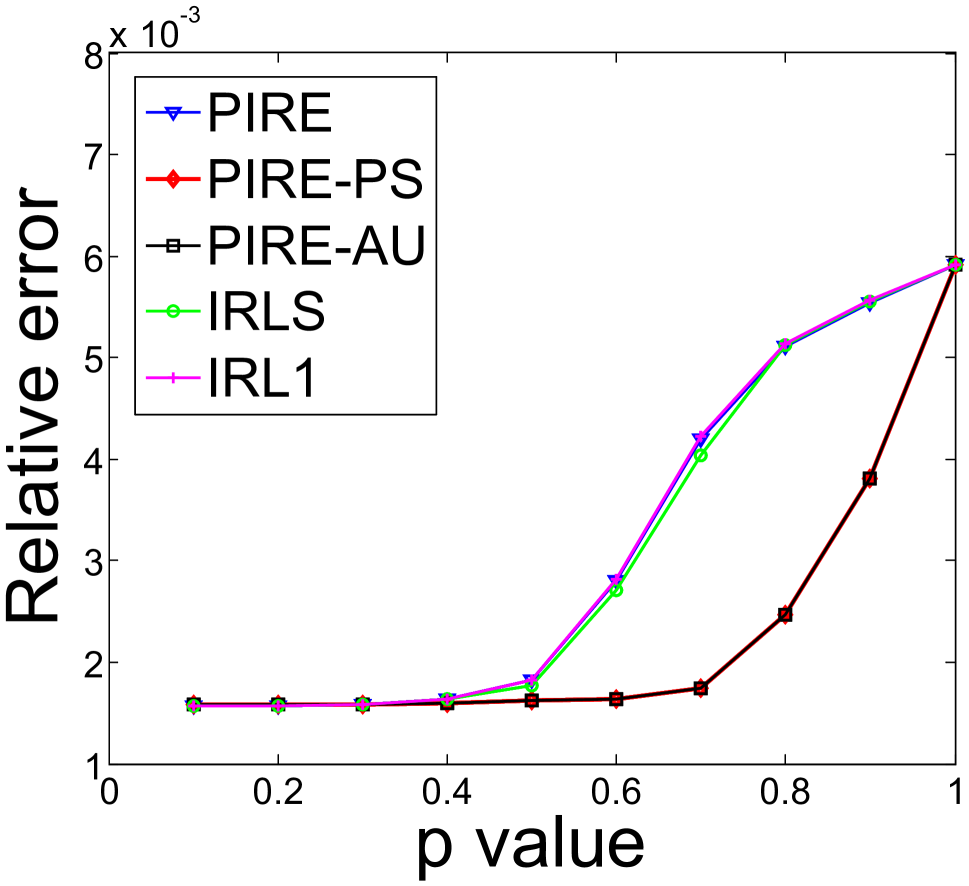
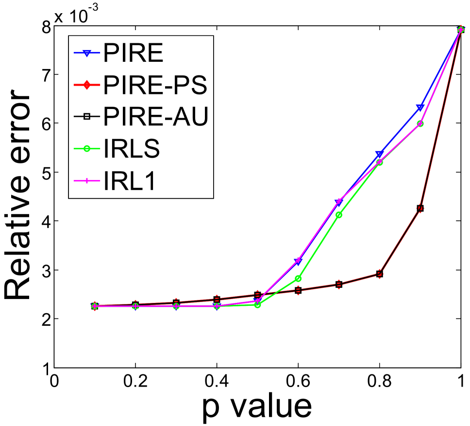
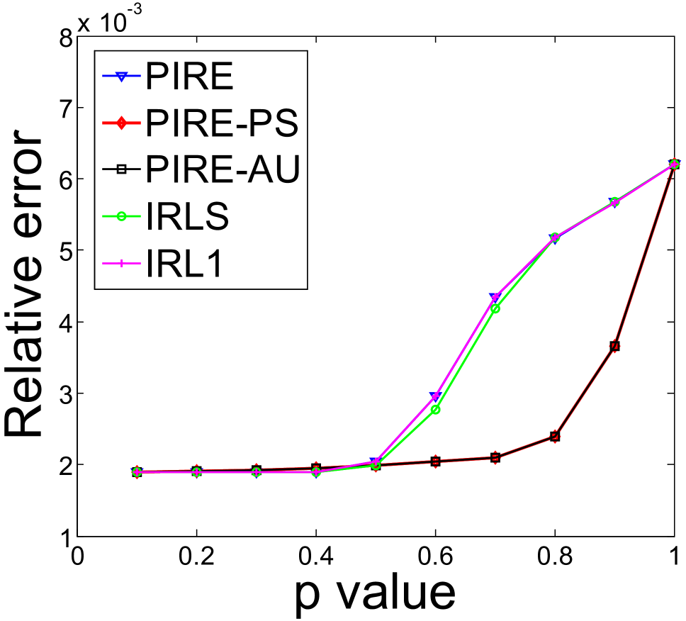
Figure 1: Recovery performance comparison with a different number of measurement π€βˆˆβ„mΓ—1000𝐀superscriptβ„π‘š1000\mathbf{A}\in\mathbb{R}^{m\times 1000}: (a) m=200π‘š200m=200; (b) m=300π‘š300m=300; and (c) m=400π‘š400m=400.

Experiments

We present several numerical experiments to demonstrate the effectiveness of the proposed PIRE algorithm and its splitting versions. All the algorithms are implemented by Matlab, and are tested on a PC with 8 GB of RAM and Intel Core 2 Quad CPU Q9550.

β„“psubscriptℓ𝑝\ell_{p}-Minimization

We compare our proposed PIRE, PIRE-PS and PIRE-AU algorithms with IRLS and IRL1 for solving the β„“psubscriptℓ𝑝\ell_{p}-minimization problem (7). For fair comparison, we try to use the same settings of all the completed algorithms. We use the solution to the β„“1subscriptβ„“1\ell_{1}-minimization problem as the initialization. We find that this will accelerate the convergence of the iteratively reweighted algorithms, and also enhance the recovery performance. The choice of Ο΅italic-Ο΅\epsilon in (8) and (10) plays an important role for sparse signal recovery, but theoretical support has not been carried out so far. Several different decreasing rules have been tested before (?;Β ?;Β ?), but none of them dominates others. Since the sparsity of sparse signal is usually unknown, we empirically set Ο΅k+1=Ο΅k/ρsuperscriptitalic-Ο΅π‘˜1superscriptitalic-Ο΅π‘˜πœŒ\epsilon^{k+1}=\epsilon^{k}/\rho, with Ο΅0=0.01superscriptitalic-Ο΅00.01\epsilon^{0}=0.01, and ρ=1.1𝜌1.1\rho=1.1 (?). The algorithms are stopped when ‖𝐱kβˆ’π±k+1β€–2/‖𝐱kβ€–2≀10βˆ’6subscriptnormsuperscriptπ±π‘˜superscriptπ±π‘˜12subscriptnormsuperscriptπ±π‘˜2superscript106||\mathbf{x}^{k}-\mathbf{x}^{k+1}||_{2}/||\mathbf{x}^{k}||_{2}\leq 10^{-6}.

IRL1 requires solving (9) as inner loop. FISTA is employed to solve (9) with warm start, i.e. using 𝐱ksuperscriptπ±π‘˜\mathbf{x}^{k} as initialization to obtain 𝐱k+1superscriptπ±π‘˜1\mathbf{x}^{k+1}. This trick greatly reduces the inner loop iteration, which is the main cost for IRL1. For PIRE-PS and PIRE-AU algorithms, we solve problem (29) by setting S=20𝑆20S=20.

Table 1: Comparison of iteration number, running time (in seconds), objective function value and relative recovery error of different iterative reweighted methods.
Size (m,n,tπ‘šπ‘›π‘‘m,n,t) Methods Iter. Time Obj. Recovery error
(second). (Γ—10βˆ’2absentsuperscript102\times 10^{-2}) (Γ—10βˆ’3absentsuperscript103\times 10^{-3})
(100,500,50) PIRE 116 0. 70 5.238 2.529
PIRE-PS 58 0. 48 5.239 2.632
PIRE-AU 56 0. 63 5.239 2.632
IRLS 168 81. 82 5.506 2.393
IRL1 56 3. 43 5.239 2.546
(200,800,100) PIRE 119 1. 48 16.923 2.246
PIRE-PS 37 0. 82 16.919 2.192
PIRE-AU 36 0. 88 16.919 2.192
IRLS 169 474. 19 17.784 2.142
IRL1 81 13. 53 16.924 2.248
(300,1000,200) PIRE 151 4. 63 42.840 2.118
PIRE-PS 29 1. 38 42.815 1.978
PIRE-AU 28 1. 34 42.815 1.977
IRLS 171 1298. 70 44.937 2.015
IRL1 79 35. 59 42.844 2.124
(500,1500,200) PIRE 159 8. 88 64.769 2.010
PIRE-PS 26 2. 27 64.718 1.814
PIRE-AU 25 2. 20 64.718 1.814
IRLS 171 3451. 79 67.996 1.923
IRL1 89 80. 89 64.772 2.013
( 800,2000,200) PIRE 140 14. 99 87.616 1.894
PIRE-PS 33 5. 15 87.533 1.648
PIRE-AU 32 4. 97 87.533 1.648
IRLS 177 7211. 2 91.251 1.851
IRL1 112 173. 26 87.617 1.895

Sparse Signal Recovery

The first experiment is to examine the recovery performance of sparse signals by using the proposed methods. The setup for each trial is as follows. The dictionary π€βˆˆβ„mΓ—n𝐀superscriptβ„π‘šπ‘›\mathbf{A}\in\mathbb{R}^{m\times n} is a Gaussian random matrix generated by Matlab command dn, with the sizes m=200,300,400π‘š200300400m=200,300,400, and n=1000𝑛1000n=1000. The sparse signal 𝐱𝐱\mathbf{x} is randomly generated with sparsity ‖𝐱‖0=20subscriptnorm𝐱020||\mathbf{x}||_{0}=20. The response 𝐛=𝐀𝐱+0.01β€‹πžπ›π€π±0.01𝐞\mathbf{b}=\mathbf{A}\mathbf{x}+0.01\mathbf{e}, where 𝐞𝐞\mathbf{e} is Gaussian random vector. Given 𝐀𝐀\mathbf{A} and 𝐛𝐛\mathbf{b}, we can recover 𝐱^^𝐱\hat{\mathbf{x}} by solving the β„“psubscriptℓ𝑝\ell_{p}-minimization problem by different methods. The parameter is set to Ξ»=10βˆ’4πœ†superscript104\lambda=10^{-4}. We use the relative recovery error ‖𝐱^βˆ’π±β€–2/‖𝐱‖2subscriptnorm^𝐱𝐱2subscriptnorm𝐱2||\hat{\mathbf{x}}-\mathbf{x}||_{2}/||\mathbf{x}||_{2} to measure the recovery performance. Based on the above settings and generated data, we find that the recovery performances are stable. We run 20 trials and report the mean relative error for comparison.

Figure 1 plots the relative recovery errors v.s. different p𝑝p values (p=0.1,β‹―,0.9,1𝑝0.1β‹―0.91p=0.1,\cdots,0.9,1) on three data sets with different numbers of measurements. The result for p=1𝑝1p=1 is obtained by FISTA for β„“1subscriptβ„“1\ell_{1}-minimization. We can see that all the iteratively reweighted algorithms achieve better recovery performance with p<1𝑝1p<1 than β„“1subscriptβ„“1\ell_{1}-minimization. Also a smaller value of p𝑝p leads to better recovery performance, though the β„“psubscriptℓ𝑝\ell_{p}-minimization problem is nonconvex and a globally optimal solution is not available. In most cases, PIRE is comparative with IRLS and IRL1. A surprising result is that PIRE-PS and PIRE-AU outperform the other methods when 0.5<p<10.5𝑝10.5<p<1. They use a smaller Lipschitz constant than PIRE, and thus may converge faster. But none of these iteratively reweighted methods is guaranteed to be optimal.
Refer to caption
(a)
Refer to caption
(b)
Refer to caption
(c)
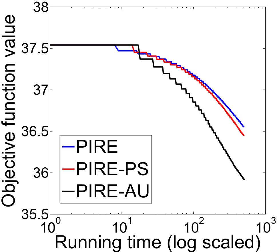
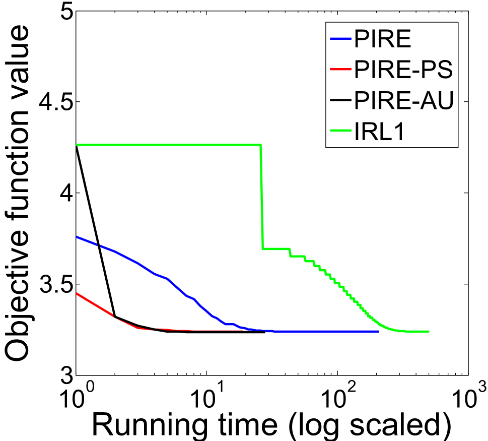
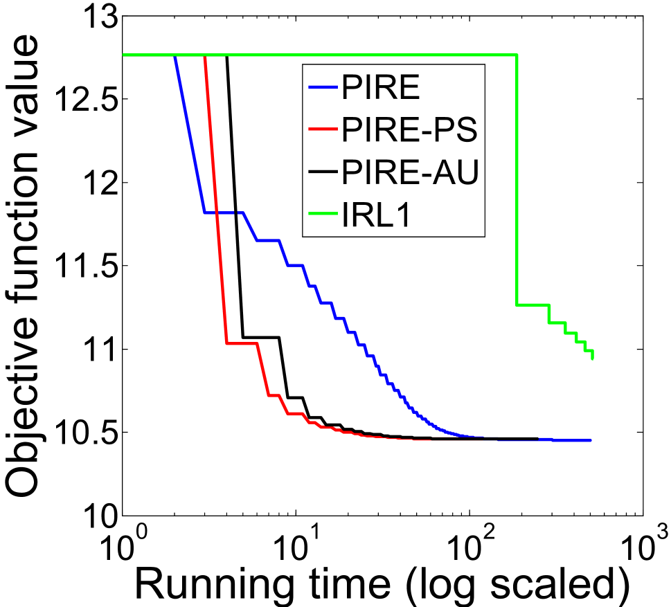
Figure 2: Running time v.s. objective function value on three synthesis data sets with size (m,n,t)π‘šπ‘›π‘‘(m,n,t): (a) (1000,3000,500); (b) (1000,5000,1000); (c) (1000,10000,1000).

Running Time Comparison

The second experiment is to show the advantage in running time of the proposed methods. We implement all the completed methods in matrix form for solving the following β„“psubscriptℓ𝑝\ell_{p}-minimization problem

minπ—βˆˆβ„nΓ—t⁑λ​‖𝐗‖pp+12β€‹β€–π€π—βˆ’πβ€–F2,subscript𝐗superscriptβ„π‘›π‘‘πœ†superscriptsubscriptnorm𝐗𝑝𝑝12superscriptsubscriptnorm𝐀𝐗𝐁𝐹2\min_{\mathbf{X}\in\mathbb{R}^{n\times t}}\lambda||\mathbf{X}||_{p}^{p}+\frac{1}{2}||\mathbf{A}\mathbf{X}-\mathbf{B}||_{F}^{2}, (36)

where π€βˆˆβ„mΓ—n𝐀superscriptβ„π‘šπ‘›\mathbf{A}\in\mathbb{R}^{m\times n} and πβˆˆβ„mΓ—t𝐁superscriptβ„π‘šπ‘‘\mathbf{B}\in\mathbb{R}^{m\times t}, ‖𝐗‖pp=βˆ‘i​j|Xi​j|psuperscriptsubscriptnorm𝐗𝑝𝑝subscript𝑖𝑗superscriptsubscript𝑋𝑖𝑗𝑝||\mathbf{X}||_{p}^{p}=\sum_{ij}|X_{ij}|^{p}, and p𝑝p is set to 0.5 in this test. 𝐀𝐀\mathbf{A}, 𝐁𝐁\mathbf{B} and 𝐗𝐗\mathbf{X} are generated by the same procedure as the above section, and the same settings of algorithm parameters are followed. Each column of 𝐗𝐗\mathbf{X} is with sparsity nΓ—2%𝑛percent2n\times 2\%. We test on several different sizes of data sets, parameterized as (m,n,t)π‘šπ‘›π‘‘(m,n,t). The iteration number, running time, objective function value and the relative recovery error are tabulated in Table 1. It can be seen that the proposed methods are much more efficient than IRLS and IRL1. PIRE-PS and PIRE-AU converge with less iteration and less running time. In our test, IRL1 is more efficient than IRLS. The reasons lie in: (1) initialization as a sparse solution to β„“1subscriptβ„“1\ell_{1}-minimization is a good choice for IRL1, but not for IRLS; (2) For each iteration in IRLS, solving t𝑑t equations (11) in a loop by Matlab is not efficient; (3) IRL1 converges with less inner loop iterations due to warm start.

We also plot the running time v.s. objective function value on three larger data sets in Figure 2. The algorithms are stopped within 500 seconds in this test. IRLS costs much more time, and thus it is not plotted. IRL1 is not plotted for the case n=10,000𝑛10000n=10,000. It can be seen that PIRE-PS and PIRE-AU decreases the objective function value faster than PIRE.

Multi-Task Feature Learning

In this experiment, we use our methods to solve the multi-task learning problem. Assume we are given mπ‘šm learning tasks associated with {(𝐗1,𝐲1),β‹―,(𝐗m,𝐲m)}subscript𝐗1subscript𝐲1β‹―subscriptπ—π‘šsubscriptπ²π‘š\{(\mathbf{X}_{1},\mathbf{y}_{1}),\cdots,(\mathbf{X}_{m},\mathbf{y}_{m})\}, where 𝐗iβˆˆβ„niΓ—dsubscript𝐗𝑖superscriptℝsubscript𝑛𝑖𝑑\mathbf{X}_{i}\in\mathbb{R}^{n_{i}\times d} is the data matrix of the i𝑖i-th task with each row a sample, 𝐲iβˆˆβ„nisubscript𝐲𝑖superscriptℝsubscript𝑛𝑖\mathbf{y}_{i}\in\mathbb{R}^{n_{i}} is the label of the i𝑖i-th task, nisubscript𝑛𝑖n_{i} is the number of samples for the i𝑖i-th task, and d𝑑d is the data dimension. Our goal is to find a matrix 𝐙=[𝐳1,β‹―,𝐳m]βˆˆβ„dΓ—m𝐙subscript𝐳1β‹―subscriptπ³π‘šsuperscriptβ„π‘‘π‘š\mathbf{Z}=[\mathbf{z}_{1},\cdots,\mathbf{z}_{m}]\in\mathbb{R}^{d\times m} such that 𝐲iβ‰ˆπ—i​𝐳isubscript𝐲𝑖subscript𝐗𝑖subscript𝐳𝑖\mathbf{y}_{i}\approx\mathbf{X}_{i}\mathbf{z}_{i}. The capped-β„“1subscriptβ„“1\ell_{1} norm is used to regularize 𝐙𝐙\mathbf{Z} (?)

minπ™β‘Ξ»β€‹βˆ‘j=1dmin⁑(‖𝐳jβ€–1,ΞΈ)+h​(𝐙),subscriptπ™πœ†superscriptsubscript𝑗1𝑑subscriptnormsuperscript𝐳𝑗1πœƒβ„Žπ™\min_{\mathbf{Z}}\lambda\sum_{j=1}^{d}\min(||\mathbf{z}^{j}||_{1},\theta)+h(\mathbf{Z}), (37)

where h​(𝐙)=βˆ‘i=1m‖𝐗i​𝐳iβˆ’π²iβ€–22/m​niβ„Žπ™superscriptsubscript𝑖1π‘šsuperscriptsubscriptnormsubscript𝐗𝑖subscript𝐳𝑖subscript𝐲𝑖22π‘šsubscript𝑛𝑖h(\mathbf{Z})=\sum_{i=1}^{m}||\mathbf{X}_{i}\mathbf{z}_{i}-\mathbf{y}_{i}||_{2}^{2}/mn_{i} is the loss function, ΞΈ>0πœƒ0\theta>0 is the thresholding parameter, and 𝐳jsuperscript𝐳𝑗\mathbf{z}^{j} is the j𝑗j-th row of 𝐙𝐙\mathbf{Z}. The above problem can be solved by our proposed PIRE, PIRE-PS and PIRE-AU algorithms, by letting f​(𝐲)=βˆ‘j=1dmin⁑(yi,ΞΈ)𝑓𝐲superscriptsubscript𝑗1𝑑subscriptπ‘¦π‘–πœƒf(\mathbf{y})=\sum_{j=1}^{d}\min(y_{i},\theta), and g​(𝐙)=[‖𝐳1β€–1;β‹―;‖𝐳mβ€–1]𝑔𝐙subscriptnormsuperscript𝐳11β‹―subscriptnormsuperscriptπ³π‘š1g(\mathbf{Z})=[||\mathbf{z}^{1}||_{1};\cdots;||\mathbf{z}^{m}||_{1}].

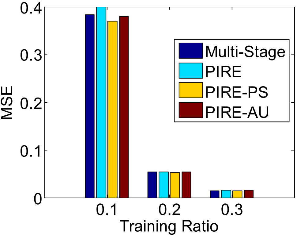
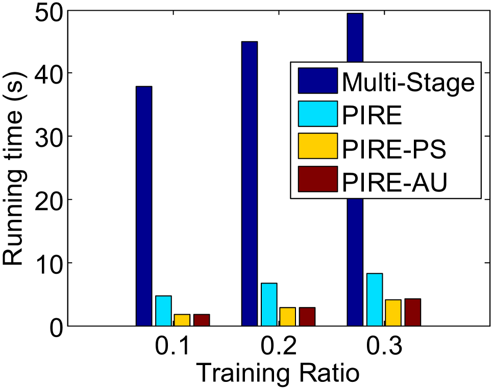
The Isolet (?) data set is used in our test. 150 subjects spoke the name of each letter of the alphabet twice. Hence, we have 52 training examples from each speaker. The speakers are grouped into 5 subsets of 30 speakers each. Thus, we have 5 tasks with each task corresponding to a subset. There are 1560, 1560, 1560, 1558, and 1559 samples of 5 tasks, respectively. The data dimension is 617, and the response is the English letter label (1-26). We randomly select the training samples from each task with different training ratios (0.1, 0.2 and 0.3) and use the rest of samples to form the test set. We compare our PIRE, PIRE-PS and PIRE-AU (we set S=m=5π‘†π‘š5S=m=5 in PIRE-PS and PIRE-AU) with the Multi-Stage algorithm (?). We report the Mean Squared Error (MSE) on the test set and the running time for solving (37) on the training set. The results are averaged over 10 random splittings. As shown in Figure 3, it can be seen that all these methods achieve comparative performance, but our PIRE, PIRE-PS and PIRE-AU are much more efficient than the Multi-Stage algorithm.
Refer to caption
(a)
Refer to caption
(b)
Figure 3: Comparison of (a) mean squared error (MSE) and running time on the Isolet data set for multi-task feature learning.

Conclusions

This paper proposes the PIRE algorithm for solving the general problem (1). PIRE solves a series of problem (2), whose computational cost is usually very cheap. We further propose two splitting versions of PIRE to handle the multi-variable problems. In theory, we prove that PIRE (also its splitting versions) converges and any limit point is a stationary point. We test our methods to solve the β„“psubscriptℓ𝑝\ell_{p}-minimization problem and multi-task feature learning problem. Experimental results on both synthesis and real data sets show that our methods are with comparative learning performance, but much more efficient, by comparing with IRLS and IRL1 or multi-stage algorithms. It would be interesting to apply PIRE for structured sparsity optimization, and also the nonconvex low rank regularized minimization problems (?).

Acknowledgements

This research is supported by the Singapore National Research Foundation under its International Research Centre @Singapore Funding Initiative and administered by the IDM Programme Office. Z. Lin is supported by NSF of China (Grant nos. 61272341, 61231002, and 61121002) and MSRA.

References

  • [Bache and Lichman 2013] Bache, K., and Lichman, M. 2013. UCI machine learning repository. http://archive.ics.uci.edu/ml.
  • [Beck and Teboulle 2009] Beck, A., and Teboulle, M. 2009. A fast iterative shrinkage-thresholding algorithm for linear inverse problems. SIAM Journal on Imaging Sciences 2(1):183–202.
  • [Bertsekas 1999] Bertsekas, D.Β P. 1999. Nonlinear programming. Athena Scientific (Belmont, Mass.), 2nd edition.
  • [CandΓ¨s, Wakin, and Boyd 2008] CandΓ¨s, E.; Wakin, M.; and Boyd, S. 2008. Enhancing sparsity by reweighted β„“1subscriptβ„“1\ell_{1} minimization. Journal of Fourier Analysis and Applications 14(5):877–905.
  • [Chen and Zhou ] Chen, X., and Zhou, W. Convergence of the reweighted β„“1subscriptβ„“1\ell_{1} minimization algorithm for β„“2βˆ’β„“psubscriptβ„“2subscriptℓ𝑝\ell_{2}-\ell_{p} minimization. to appear in Comp. Optim. Appl.
  • [Clarke 1983] Clarke, F.Β H. 1983. Nonsmooth analysis and optimization. In Proceedings of the International Congress of Mathematicians (Helsinki, 1978), 847–853.
  • [Fan and Li 2001] Fan, J., and Li, R. 2001. Variable selection via nonconcave penalized likelihood and its oracle properties. Journal of the American Statistical Association 96(456):1348–1360.
  • [Gong et al. 2013] Gong, P.; Zhang, C.; Lu, Z.; Huang, J.; and Ye, J. 2013. A general iterative shrinkage and thresholding algorithm for non-convex regularized optimization problems. ICML.
  • [Gong, Ye, and Zhang 2012a] Gong, P.; Ye, J.; and Zhang, C. 2012a. Multi-stage multi-task feature learning. In NIPS.
  • [Gong, Ye, and Zhang 2012b] Gong, P.; Ye, J.; and Zhang, C. 2012b. Robust multi-task feature learning. In ACM SIGKDD, 895–903. ACM.
  • [Jacob, Obozinski, and Vert 2009] Jacob, L.; Obozinski, G.; and Vert, J.-P. 2009. Group Lasso with overlap and graph Lasso. In ICML, 433–440. ACM.
  • [Knight and Fu 2000] Knight, K., and Fu, W. 2000. Asymptotics for Lasso-type estimators. Annals of Statistics 1356–1378.
  • [Lai, Xu, and Yin 2013] Lai, M.-J.; Xu, Y.; and Yin, W. 2013. Improved iteratively reweighted least squares for unconstrained smoothed β„“qsubscriptβ„“π‘ž\ell_{q} minimization. SIAM Journal on Numerical Analysis 51(2):927–957.
  • [Liu, Lin, and Su 2013] Liu, R.; Lin, Z.; and Su, Z. 2013. Linearized alternating direction method with parallel splitting and adaptive penalty for separable convex programs in machine learning. In ACML.
  • [Lu et al. 2014] Lu, C.; Tang, J.; Lin, Z.; and Yan, S. 2014. Generalized nonconvex nonsmooth low-rank minimization. In CVPR.
  • [Lu 2012] Lu, Z. 2012. Iterative reweighted minimization methods for β„“psubscriptℓ𝑝\ell_{p} regularized unconstrained nonlinear programming. Mathematical Programming.
  • [Mohan and Fazel 2012] Mohan, K., and Fazel, M. 2012. Iterative reweighted algorithms for matrix rank minimization. In JMLR, volumeΒ 13, 3441–3473.
  • [Wright et al. 2009] Wright, J.; Yang, A.Β Y.; Ganesh, A.; Sastry, S.Β S.; and Ma, Y. 2009. Robust face recognition via sparse representation. TPAMI 31(2):210–227.
  • [Zhang 2008] Zhang, T. 2008. Multi-stage convex relaxation for learning with sparse regularization. In NIPS, 1929–1936.
  • [Zhang 2010] Zhang, C. 2010. Nearly unbiased variable selection under minimax concave penalty. The Annals of Statistics.
  • [Zhou et al. 2010] Zhou, Z.; Li, X.; Wright, J.; CandΓ¨s, E.; and Ma, Y. 2010. Stable principal component pursuit. In IEEE International Symposium on Information Theory Proceedings, 1518–1522. IEEE.
  • [Zuo and Lin 2011] Zuo, W., and Lin, Z. 2011. A generalized accelerated proximal gradient approach for total-variation-based image restoration. TIP 20(10):2748–2759.

Supplementary Material of
Proximal Iteratively Reweighted Algorithm with Multiple Splitting for Nonconvex Sparsity Optimization

Canyi Lu1, Yunchao Wei2, Zhouchen Lin3,⋆⋆\star⋆⋆\star⋆⋆\starCorresponding author., Shuicheng Yan1
1
Department of Electrical and Computer Engineering, National University of Singapore

2 Institute of Information Science, Beijing Jiaotong University

3 Key Laboratory of Machine Perception (MOE), School of EECS, Peking University

canyilu@gmail.com, wychao1987@gmail.com, zlin@pku.edu.cn, eleyans@nus.edu.sg

In this supplementary material, we give the detailed convergence results and proofs of the PIRE-PS and PIRE-AU algorithms.

Proof of Theorem 2

Proof. The sequence {𝐱k}superscriptπ±π‘˜\{\mathbf{x}^{k}\} generated in Algorithm 1 is bounded by Theorem 1. Hence, there exists an accumulation point π±βˆ—superscript𝐱\mathbf{x}^{*}, and a subsequence {𝐱kj}superscript𝐱subscriptπ‘˜π‘—\{\mathbf{x}^{k_{j}}\} such that limjβ†’βˆžπ±kj=π±βˆ—subscript→𝑗superscript𝐱subscriptπ‘˜π‘—superscript𝐱\lim\limits_{j\rightarrow\infty}\mathbf{x}^{k_{j}}=\mathbf{x}^{*}. From the fact that limkβ†’βˆž(𝐱kβˆ’π±k+1)=𝟎subscriptβ†’π‘˜superscriptπ±π‘˜superscriptπ±π‘˜10\lim\limits_{k\rightarrow\infty}(\mathbf{x}^{k}-\mathbf{x}^{k+1})=\bm{0} in Theorem 1, we have limjβ†’βˆžπ±kj+1=π±βˆ—subscript→𝑗superscript𝐱subscriptπ‘˜π‘—1superscript𝐱\lim\limits_{j\rightarrow\infty}\mathbf{x}^{k_{j}+1}=\mathbf{x}^{*}. Since 𝐱kj+1superscript𝐱subscriptπ‘˜π‘—1\mathbf{x}^{k_{j}+1} solves problem (18), there exists 𝐯kj+1βˆˆβˆ‚βŸ¨π°kj,𝐠​(𝐱kj+1)⟩superscript𝐯subscriptπ‘˜π‘—1superscript𝐰subscriptπ‘˜π‘—π superscript𝐱subscriptπ‘˜π‘—1\mathbf{v}^{k_{j}+1}\in\partial\langle\mathbf{w}^{k_{j}},\mathbf{g}(\mathbf{x}^{k_{j}+1})\rangle such that

λ​𝐯kj+1+βˆ‡h​(𝐱kj)+μ​(𝐱kj+1βˆ’π±kj)=𝟎.πœ†superscript𝐯subscriptπ‘˜π‘—1βˆ‡β„Žsuperscript𝐱subscriptπ‘˜π‘—πœ‡superscript𝐱subscriptπ‘˜π‘—1superscript𝐱subscriptπ‘˜π‘—0\lambda\mathbf{v}^{k_{j}+1}+\nabla h(\mathbf{x}^{k_{j}})+\mu(\mathbf{x}^{k_{j}+1}-\mathbf{x}^{k_{j}})=\mathbf{0}. (38)

By the upper semi-continuous property of the subdifferential (?), there exists π―βˆ—βˆˆβˆ‚βŸ¨π°βˆ—,𝐠​(π±βˆ—)⟩superscript𝐯superscript𝐰𝐠superscript𝐱\mathbf{v}^{*}\in\partial\langle\mathbf{w}^{*},\mathbf{g}(\mathbf{x}^{*})\rangle, with π°βˆ—βˆˆβˆ’βˆ‚(βˆ’f​(𝐠​(π±βˆ—)))superscript𝐰𝑓𝐠superscript𝐱\mathbf{w}^{*}\in-\partial\left(-f(\mathbf{g}(\mathbf{x}^{*}))\right), such that

𝟎=Ξ»β€‹π―βˆ—+βˆ‡h​(π±βˆ—)βˆˆβˆ‚F​(π±βˆ—)βˆ‚π±βˆ—.0πœ†superscriptπ―βˆ‡β„Žsuperscript𝐱𝐹superscript𝐱superscript𝐱\mathbf{0}=\lambda\mathbf{v}^{*}+\nabla h(\mathbf{x}^{*})\in\frac{\partial F(\mathbf{x}^{*})}{\partial\mathbf{x}^{*}}. (39)

Hence π±βˆ—superscript𝐱\mathbf{x}^{*} is a stationary point of (1).

Furthermore, summing (25) for k=1,β‹―,nπ‘˜1⋯𝑛k=1,\cdots,n, we have

F​(𝐱1)βˆ’F​(𝐱n+1)β‰₯(ΞΌβˆ’L​(h)2)β€‹βˆ‘k=1n‖𝐱k+1βˆ’π±kβ€–22β‰₯n​(ΞΌβˆ’L​(h)2)​min1≀k≀n​‖𝐱k+1βˆ’π±kβ€–22.𝐹superscript𝐱1𝐹superscript𝐱𝑛1πœ‡πΏβ„Ž2superscriptsubscriptπ‘˜1𝑛superscriptsubscriptnormsuperscriptπ±π‘˜1superscriptπ±π‘˜22π‘›πœ‡πΏβ„Ž2subscript1π‘˜π‘›superscriptsubscriptnormsuperscriptπ±π‘˜1superscriptπ±π‘˜22\begin{split}F(\mathbf{x}^{1})-F(\mathbf{x}^{n+1})&\geq\left(\mu-\frac{L(h)}{2}\right)\sum_{k=1}^{n}||\mathbf{x}^{k+1}-\mathbf{x}^{k}||_{2}^{2}\\ &\geq n\left(\mu-\frac{L(h)}{2}\right)\min_{1\leq k\leq n}||\mathbf{x}^{k+1}-\mathbf{x}^{k}||_{2}^{2}.\end{split} (40)

Thus

min1≀k≀n​‖𝐱k+1βˆ’π±kβ€–22≀F​(𝐱1)βˆ’F​(𝐱n+1)n​(ΞΌβˆ’L​(h)2)≀F​(𝐱1)βˆ’F​(π±βˆ—)n​(ΞΌβˆ’L​(h)2).subscript1π‘˜π‘›superscriptsubscriptnormsuperscriptπ±π‘˜1superscriptπ±π‘˜22𝐹superscript𝐱1𝐹superscript𝐱𝑛1π‘›πœ‡πΏβ„Ž2𝐹superscript𝐱1𝐹superscriptπ±π‘›πœ‡πΏβ„Ž2\begin{split}\min_{1\leq k\leq n}||\mathbf{x}^{k+1}-\mathbf{x}^{k}||_{2}^{2}\leq&\frac{F(\mathbf{x}^{1})-F(\mathbf{x}^{n+1})}{n\left(\mu-\frac{L(h)}{2}\right)}\\ \leq&\frac{F(\mathbf{x}^{1})-F(\mathbf{x}^{*})}{n\left(\mu-\frac{L(h)}{2}\right)}.\end{split} (41)

β– β– \hfill\blacksquare

Convergence Analysis of PIRE-PS

For the general PIRE-PS algorithm for solving problem (29) by (30) and (31), actually its updating rule is the same as PIRE. Thus the same convergence results in Theorem 1 and 2 hold. In this section, we provide the convergence analysis of PIRE-PS algorithm by (32) and (31) for solving problem (29) with the squared loss function h​(𝐱1,β‹―,𝐱S)=12β€‹β€–βˆ‘s=1S𝐀s​𝐱sβˆ’π›β€–22β„Žsubscript𝐱1β‹―subscript𝐱𝑆12superscriptsubscriptnormsuperscriptsubscript𝑠1𝑆subscript𝐀𝑠subscript𝐱𝑠𝐛22h(\mathbf{x}_{1},\cdots,\mathbf{x}_{S})=\frac{1}{2}\left\|\sum_{s=1}^{S}\mathbf{A}_{s}\mathbf{x}_{s}-\mathbf{b}\right\|_{2}^{2}.

Theorem 3.

Assume that the squared loss function h​(𝐱1,β‹―,𝐱S)=12β€‹β€–βˆ‘s=1S𝐀s​𝐱sβˆ’π›β€–22β„Žsubscript𝐱1β‹―subscript𝐱𝑆12superscriptsubscriptnormsuperscriptsubscript𝑠1𝑆subscript𝐀𝑠subscript𝐱𝑠𝐛22h(\mathbf{x}_{1},\cdots,\mathbf{x}_{S})=\frac{1}{2}\left\|\sum_{s=1}^{S}\mathbf{A}_{s}\mathbf{x}_{s}-\mathbf{b}\right\|_{2}^{2} is used in problem (29). Let D=F​(𝐱1)𝐷𝐹superscript𝐱1D=F(\mathbf{x}^{1}), and ΞΌs>‖𝐀sβ€–222subscriptπœ‡π‘ superscriptsubscriptnormsubscript𝐀𝑠222\mu_{s}>\frac{||\mathbf{A}_{s}||_{2}^{2}}{2}, s=1,β‹―,S𝑠1⋯𝑆s=1,\cdots,S, and Ξ΄=mins⁑{ΞΌsβˆ’β€–π€sβ€–22/2}𝛿subscript𝑠subscriptπœ‡π‘ superscriptsubscriptnormsubscript𝐀𝑠222\delta=\min_{s}\{\mu_{s}-||\mathbf{A}_{s}||_{2}^{2}/2\}. The sequence {𝐱k}superscriptπ±π‘˜\{\mathbf{x}^{k}\} generated by PIRE-PS in (32) and (31) satisfies the following properties:

  1. (1)

    F​(𝐱k)𝐹superscriptπ±π‘˜F(\mathbf{x}^{k}) is monotonically decreasing, i.e. F​(𝐱k+1)≀F​(𝐱k)𝐹superscriptπ±π‘˜1𝐹superscriptπ±π‘˜F(\mathbf{x}^{k+1})\leq F(\mathbf{x}^{k}). Indeed,

    F​(𝐱k)βˆ’F​(𝐱k+1)β‰₯βˆ‘s=1S(ΞΌsβˆ’β€–π€sβ€–222)​‖𝐱sk+1βˆ’π±skβ€–2β‰₯0;𝐹superscriptπ±π‘˜πΉsuperscriptπ±π‘˜1superscriptsubscript𝑠1𝑆subscriptπœ‡π‘ superscriptsubscriptnormsubscript𝐀𝑠222superscriptnormsuperscriptsubscriptπ±π‘ π‘˜1superscriptsubscriptπ±π‘ π‘˜20F(\mathbf{x}^{k})-F(\mathbf{x}^{k+1})\geq\sum_{s=1}^{S}\left(\mu_{s}-\frac{||\mathbf{A}_{s}||_{2}^{2}}{2}\right)||\mathbf{x}_{s}^{k+1}-\mathbf{x}_{s}^{k}||^{2}\geq 0;
  2. (2)

    The sequence {𝐱k}superscriptπ±π‘˜\{\mathbf{x}^{k}\} is bounded;

  3. (3)

    limkβ†’βˆž(𝐱kβˆ’π±k+1)=𝟎subscriptβ†’π‘˜superscriptπ±π‘˜superscriptπ±π‘˜10\lim\limits_{k\rightarrow\infty}(\mathbf{x}^{k}-\mathbf{x}^{k+1})=\bm{0}.

  4. (4)

    Any accumulation point of {𝐱k}superscriptπ±π‘˜\{\mathbf{x}^{k}\} is a stationary point π±βˆ—superscript𝐱\mathbf{x}^{*} of problem (29).

  5. (5)

    For any nβ‰₯1𝑛1n\geq 1, min1≀k≀n​‖𝐱k+1βˆ’π±kβ€–22≀F​(𝐱1)βˆ’F​(π±βˆ—)n​δsubscript1π‘˜π‘›superscriptsubscriptnormsuperscriptπ±π‘˜1superscriptπ±π‘˜22𝐹superscript𝐱1𝐹superscript𝐱𝑛𝛿\min_{1\leq k\leq n}||\mathbf{x}^{k+1}-\mathbf{x}^{k}||_{2}^{2}\leq\frac{F(\mathbf{x}^{1})-F(\mathbf{x}^{*})}{n\delta}.

Proof. Since 𝐱sk+1subscriptsuperscriptπ±π‘˜1𝑠\mathbf{x}^{k+1}_{s} is the globally optimal solution to problem (32), the zero vector is contained in the subgradient with respect to 𝐱ssubscript𝐱𝑠\mathbf{x}_{s}. That is, there exists 𝐯sk+1βˆˆβˆ‚βŸ¨π°sk,𝐠​(𝐱sk+1)⟩superscriptsubscriptπ―π‘ π‘˜1superscriptsubscriptπ°π‘ π‘˜π subscriptsuperscriptπ±π‘˜1𝑠\mathbf{v}_{s}^{k+1}\in\partial\langle\mathbf{w}_{s}^{k},\mathbf{g}(\mathbf{x}^{k+1}_{s})\rangle such that

λ​𝐯sk+1+𝐀sT​(𝐀𝐱kβˆ’π›)+ΞΌs​(𝐱sk+1βˆ’π±sk)=𝟎.πœ†subscriptsuperscriptπ―π‘˜1𝑠superscriptsubscript𝐀𝑠𝑇superscriptπ€π±π‘˜π›subscriptπœ‡π‘ subscriptsuperscriptπ±π‘˜1𝑠subscriptsuperscriptπ±π‘˜π‘ 0\lambda\mathbf{v}^{k+1}_{s}+\mathbf{A}_{s}^{T}(\mathbf{A}\mathbf{x}^{k}-\mathbf{b})+\mu_{s}(\mathbf{x}^{k+1}_{s}-\mathbf{x}^{k}_{s})=\mathbf{0}. (42)

A dot-product with 𝐱sk+1βˆ’π±sksubscriptsuperscriptπ±π‘˜1𝑠subscriptsuperscriptπ±π‘˜π‘ \mathbf{x}^{k+1}_{s}-\mathbf{x}^{k}_{s} on both sides of (42) gives

Ξ»β€‹βŸ¨π―sk+1,𝐱sk+1βˆ’π±sk⟩+βŸ¨π€π±kβˆ’π›,𝐀s​(𝐱sk+1βˆ’π±sk)⟩+ΞΌs​‖𝐱sk+1βˆ’π±skβ€–22=0.πœ†superscriptsubscriptπ―π‘ π‘˜1superscriptsubscriptπ±π‘ π‘˜1superscriptsubscriptπ±π‘ π‘˜superscriptπ€π±π‘˜π›subscript𝐀𝑠superscriptsubscriptπ±π‘ π‘˜1superscriptsubscriptπ±π‘ π‘˜subscriptπœ‡π‘ superscriptsubscriptnormsuperscriptsubscriptπ±π‘ π‘˜1superscriptsubscriptπ±π‘ π‘˜220\begin{split}\lambda\left\langle\mathbf{v}_{s}^{k+1},\mathbf{x}_{s}^{k+1}-\mathbf{x}_{s}^{k}\right\rangle+\left\langle\mathbf{A}\mathbf{x}^{k}-\mathbf{b},\mathbf{A}_{s}(\mathbf{x}_{s}^{k+1}-\mathbf{x}_{s}^{k})\right\rangle+\mu_{s}||\mathbf{x}_{s}^{k+1}-\mathbf{x}_{s}^{k}||_{2}^{2}=0.\end{split} (43)

Recalling the definition of the subgradient of the convex function, we have

⟨𝐰sk,𝐠​(𝐱sk)βˆ’π β€‹(𝐱sk+1)⟩β‰₯⟨𝐯sk+1,𝐱skβˆ’π±sk+1⟩.subscriptsuperscriptπ°π‘˜π‘ π superscriptsubscriptπ±π‘ π‘˜π superscriptsubscriptπ±π‘ π‘˜1subscriptsuperscriptπ―π‘˜1𝑠superscriptsubscriptπ±π‘ π‘˜superscriptsubscriptπ±π‘ π‘˜1\begin{split}\langle\mathbf{w}^{k}_{s},\mathbf{g}(\mathbf{x}_{s}^{k})-\mathbf{g}(\mathbf{x}_{s}^{k+1})\rangle\geq\left\langle\mathbf{v}^{k+1}_{s},\mathbf{x}_{s}^{k}-\mathbf{x}_{s}^{k+1}\right\rangle.\end{split} (44)

Combining (43) and (44) gives

Ξ»β€‹βˆ‘s=1S⟨𝐰sk,𝐠​(𝐱sk)βˆ’π β€‹(𝐱sk+1)⟩β‰₯βˆ’βˆ‘s=1SβŸ¨π€π±kβˆ’π›,𝐀s​(𝐱skβˆ’π±sk+1)⟩+βˆ‘s=1SΞΌs​‖𝐱sk+1βˆ’π±skβ€–22=βˆ’βŸ¨π€π±kβˆ’π›,𝐀​(𝐱kβˆ’π±k+1)⟩+βˆ‘s=1SΞΌs​‖𝐱sk+1βˆ’π±skβ€–22.πœ†superscriptsubscript𝑠1𝑆superscriptsubscriptπ°π‘ π‘˜π superscriptsubscriptπ±π‘ π‘˜π superscriptsubscriptπ±π‘ π‘˜1superscriptsubscript𝑠1𝑆superscriptπ€π±π‘˜π›subscript𝐀𝑠superscriptsubscriptπ±π‘ π‘˜superscriptsubscriptπ±π‘ π‘˜1superscriptsubscript𝑠1𝑆subscriptπœ‡π‘ superscriptsubscriptnormsuperscriptsubscriptπ±π‘ π‘˜1superscriptsubscriptπ±π‘ π‘˜22superscriptπ€π±π‘˜π›π€superscriptπ±π‘˜superscriptπ±π‘˜1superscriptsubscript𝑠1𝑆subscriptπœ‡π‘ superscriptsubscriptnormsuperscriptsubscriptπ±π‘ π‘˜1superscriptsubscriptπ±π‘ π‘˜22\begin{split}&\lambda\sum_{s=1}^{S}\langle\mathbf{w}_{s}^{k},\mathbf{g}(\mathbf{x}_{s}^{k})-\mathbf{g}(\mathbf{x}_{s}^{k+1})\rangle\\ \geq&-\sum_{s=1}^{S}\left\langle\mathbf{A}\mathbf{x}^{k}-\mathbf{b},\mathbf{A}_{s}(\mathbf{x}_{s}^{k}-\mathbf{x}_{s}^{k+1})\right\rangle+\sum_{s=1}^{S}\mu_{s}||\mathbf{x}_{s}^{k+1}-\mathbf{x}_{s}^{k}||_{2}^{2}\\ =&-\langle\mathbf{A}\mathbf{x}^{k}-\mathbf{b},\mathbf{A}(\mathbf{x}^{k}-\mathbf{x}^{k+1})\rangle+\sum_{s=1}^{S}\mu_{s}||\mathbf{x}_{s}^{k+1}-\mathbf{x}_{s}^{k}||_{2}^{2}.\end{split} (45)

By using the Pythagoras relation

β€–πšβˆ’πœβ€–22βˆ’β€–π›βˆ’πœβ€–22=β€–πšβˆ’π›β€–22+2β€‹βŸ¨πšβˆ’π›,π›βˆ’πœβŸ©,subscriptsuperscriptnorm𝐚𝐜22subscriptsuperscriptnormπ›πœ22subscriptsuperscriptnormπšπ›222πšπ›π›πœ||\mathbf{a}-\mathbf{c}||^{2}_{2}-||\mathbf{b}-\mathbf{c}||^{2}_{2}=||\mathbf{a}-\mathbf{b}||^{2}_{2}+2\langle\mathbf{a}-\mathbf{b},\mathbf{b}-\mathbf{c}\rangle, (46)

we get

12​(‖𝐀𝐱kβˆ’π›β€–22βˆ’β€–π€π±k+1βˆ’π›β€–22)=12​‖𝐀​(𝐱kβˆ’π±k+1)β€–22+βŸ¨π€β€‹(𝐱kβˆ’π±k+1),𝐀𝐱k+1βˆ’π›βŸ©.12superscriptsubscriptdelimited-βˆ₯βˆ₯superscriptπ€π±π‘˜π›22superscriptsubscriptdelimited-βˆ₯βˆ₯superscriptπ€π±π‘˜1𝐛2212subscriptsuperscriptdelimited-βˆ₯βˆ₯𝐀superscriptπ±π‘˜superscriptπ±π‘˜122𝐀superscriptπ±π‘˜superscriptπ±π‘˜1superscriptπ€π±π‘˜1𝐛\begin{split}&\frac{1}{2}\left(\left\|\mathbf{A}\mathbf{x}^{k}-\mathbf{b}\right\|_{2}^{2}-\left\|\mathbf{A}\mathbf{x}^{k+1}-\mathbf{b}\right\|_{2}^{2}\right)=\frac{1}{2}\left\|\mathbf{A}\left(\mathbf{x}^{k}-\mathbf{x}^{k+1}\right)\right\|^{2}_{2}+\left\langle\mathbf{A}(\mathbf{x}^{k}-\mathbf{x}^{k+1}),\mathbf{A}\mathbf{x}^{k+1}-\mathbf{b}\right\rangle.\\ \end{split} (47)

By the assumption (C1) that fssubscript𝑓𝑠f_{s} is concave, we have

fs​(𝐠s​(𝐱sk))βˆ’fs​(𝐠s​(𝐱sk+1))β‰₯⟨𝐰sk,𝐠s​(𝐱sk)βˆ’π s​(𝐱sk+1)⟩.subscript𝑓𝑠subscript𝐠𝑠superscriptsubscriptπ±π‘ π‘˜subscript𝑓𝑠subscript𝐠𝑠superscriptsubscriptπ±π‘ π‘˜1superscriptsubscriptπ°π‘ π‘˜subscript𝐠𝑠superscriptsubscriptπ±π‘ π‘˜subscript𝐠𝑠superscriptsubscriptπ±π‘ π‘˜1f_{s}(\mathbf{g}_{s}(\mathbf{x}_{s}^{k}))-f_{s}(\mathbf{g}_{s}(\mathbf{x}_{s}^{k+1}))\geq\langle\mathbf{w}_{s}^{k},\mathbf{g}_{s}(\mathbf{x}_{s}^{k})-\mathbf{g}_{s}(\mathbf{x}_{s}^{k+1})\rangle. (48)

Now, combining (45)(47) and (48) leads to

F​(𝐱k)βˆ’F​(𝐱k+1)=Ξ»β€‹βˆ‘s=1S(fs​(𝐠s​(𝐱sk))βˆ’fs​(𝐠s​(𝐱sk+1)))+12​(‖𝐀𝐱kβˆ’π›β€–22βˆ’β€–π€π±k+1βˆ’π›β€–22)β‰₯βˆ’βŸ¨π€π±kβˆ’π›,𝐀​(𝐱kβˆ’π±k+1)⟩+βˆ‘s=1SΞΌs​‖𝐱sk+1βˆ’π±skβ€–22+12​‖𝐀​(𝐱kβˆ’π±k+1)β€–22+βŸ¨π€β€‹(𝐱kβˆ’π±k+1),𝐀𝐱k+1βˆ’π›βŸ©=βˆ’12​‖𝐀​(𝐱kβˆ’π±k+1)β€–22+βˆ‘s=1SΞΌs​‖𝐱sk+1βˆ’π±skβ€–22β‰₯βˆ‘s=1S(ΞΌsβˆ’β€–π€sβ€–222)​‖𝐱sk+1βˆ’π±skβ€–22β‰₯δ​‖𝐱k+1βˆ’π±kβ€–22β‰₯0,𝐹superscriptπ±π‘˜πΉsuperscriptπ±π‘˜1πœ†superscriptsubscript𝑠1𝑆subscript𝑓𝑠subscript𝐠𝑠superscriptsubscriptπ±π‘ π‘˜subscript𝑓𝑠subscript𝐠𝑠superscriptsubscriptπ±π‘ π‘˜112superscriptsubscriptdelimited-βˆ₯βˆ₯superscriptπ€π±π‘˜π›22superscriptsubscriptdelimited-βˆ₯βˆ₯superscriptπ€π±π‘˜1𝐛22superscriptπ€π±π‘˜π›π€superscriptπ±π‘˜superscriptπ±π‘˜1superscriptsubscript𝑠1𝑆subscriptπœ‡π‘ superscriptsubscriptnormsuperscriptsubscriptπ±π‘ π‘˜1superscriptsubscriptπ±π‘ π‘˜2212superscriptsubscriptdelimited-βˆ₯βˆ₯𝐀superscriptπ±π‘˜superscriptπ±π‘˜122𝐀superscriptπ±π‘˜superscriptπ±π‘˜1superscriptπ€π±π‘˜1𝐛12superscriptsubscriptdelimited-βˆ₯βˆ₯𝐀superscriptπ±π‘˜superscriptπ±π‘˜122superscriptsubscript𝑠1𝑆subscriptπœ‡π‘ superscriptsubscriptnormsuperscriptsubscriptπ±π‘ π‘˜1superscriptsubscriptπ±π‘ π‘˜22superscriptsubscript𝑠1𝑆subscriptπœ‡π‘ superscriptsubscriptnormsubscript𝐀𝑠222superscriptsubscriptnormsuperscriptsubscriptπ±π‘ π‘˜1superscriptsubscriptπ±π‘ π‘˜22𝛿superscriptsubscriptnormsuperscriptπ±π‘˜1superscriptπ±π‘˜220\begin{split}&F(\mathbf{x}^{k})-F(\mathbf{x}^{k+1})\\ =&\lambda\sum_{s=1}^{S}\left(f_{s}(\mathbf{g}_{s}(\mathbf{x}_{s}^{k}))-f_{s}(\mathbf{g}_{s}(\mathbf{x}_{s}^{k+1}))\right)+\frac{1}{2}\left(\left\|\mathbf{A}\mathbf{x}^{k}-\mathbf{b}\right\|_{2}^{2}-\left\|\mathbf{A}\mathbf{x}^{k+1}-\mathbf{b}\right\|_{2}^{2}\right)\\ \geq&-\langle\mathbf{A}\mathbf{x}^{k}-\mathbf{b},\mathbf{A}(\mathbf{x}^{k}-\mathbf{x}^{k+1})\rangle+\sum_{s=1}^{S}\mu_{s}||\mathbf{x}_{s}^{k+1}-\mathbf{x}_{s}^{k}||_{2}^{2}+\frac{1}{2}\left\|\mathbf{A}\left(\mathbf{x}^{k}-\mathbf{x}^{k+1}\right)\right\|_{2}^{2}+\left\langle\mathbf{A}(\mathbf{x}^{k}-\mathbf{x}^{k+1}),\mathbf{A}\mathbf{x}^{k+1}-\mathbf{b}\right\rangle\\ =&-\frac{1}{2}\left\|\mathbf{A}\left(\mathbf{x}^{k}-\mathbf{x}^{k+1}\right)\right\|_{2}^{2}+\sum_{s=1}^{S}\mu_{s}||\mathbf{x}_{s}^{k+1}-\mathbf{x}_{s}^{k}||_{2}^{2}\\ \geq&\sum_{s=1}^{S}\left(\mu_{s}-\frac{||\mathbf{A}_{s}||_{2}^{2}}{2}\right)||\mathbf{x}_{s}^{k+1}-\mathbf{x}_{s}^{k}||_{2}^{2}\\ \geq&\delta||\mathbf{x}^{k+1}-\mathbf{x}^{k}||_{2}^{2}\geq 0,\end{split} (49)

Thus F​(𝐱k)𝐹superscriptπ±π‘˜F(\mathbf{x}^{k}) is monotonically decreasing. Summing all the above inequalities for kβ‰₯1π‘˜1k\geq 1, it follows that

D=F​(𝐱1)β‰₯Ξ΄β€‹βˆ‘k=1βˆžβ€–π±k+1βˆ’π±kβ€–22,𝐷𝐹superscript𝐱1𝛿superscriptsubscriptπ‘˜1superscriptsubscriptnormsuperscriptπ±π‘˜1superscriptπ±π‘˜22D=F(\mathbf{x}^{1})\geq\delta\sum_{k=1}^{\infty}||\mathbf{x}^{k+1}-\mathbf{x}^{k}||_{2}^{2}, (50)

This in particular implies that limkβ†’βˆž(𝐱k+1βˆ’π±k)=𝟎subscriptβ†’π‘˜superscriptπ±π‘˜1superscriptπ±π‘˜0\lim\limits_{k\rightarrow\infty}(\mathbf{x}^{k+1}-\mathbf{x}^{k})=\mathbf{0}. Also {𝐱k}superscriptπ±π‘˜\{\mathbf{x}^{k}\} is bounded due to the condition (C4). Similar to the proof in the Theorem 2, it is easy to show that any accumulation point of {𝐱k}superscriptπ±π‘˜\{\mathbf{x}^{k}\} is a stationary point π±βˆ—superscript𝐱\mathbf{x}^{*} of problem (29). The convergence rate can be easily proved by summing (49) for k=1,β‹―,nπ‘˜1⋯𝑛k=1,\cdots,n. β– β– \hfill\blacksquare

Remark: The convergence results in the Theorem 3 is similar to that in the Theorem 1. But the main difference of the proof is that we use the Pythagoras relation (46) instead of the Lipschitz continuous property (17) of the squared loss function h​(𝐱1,β‹―,𝐱S)=12β€‹β€–βˆ‘s=1S𝐀s​𝐱sβˆ’π›β€–22β„Žsubscript𝐱1β‹―subscript𝐱𝑆12superscriptsubscriptnormsuperscriptsubscript𝑠1𝑆subscript𝐀𝑠subscript𝐱𝑠𝐛22h(\mathbf{x}_{1},\cdots,\mathbf{x}_{S})=\frac{1}{2}\left\|\sum_{s=1}^{S}\mathbf{A}_{s}\mathbf{x}_{s}-\mathbf{b}\right\|_{2}^{2}. The Pythagoras relation (46) is much tighter than (17).

Convergence Analysis of PIRE-AU

Theorem 4.

For the loss function h​(𝐱1,β‹―,𝐱S)β„Žsubscript𝐱1β‹―subscript𝐱𝑆h(\mathbf{x}_{1},\cdots,\mathbf{x}_{S}) in problem (29), assume that βˆ‡sh​(𝐱1,β‹―,𝐱S)subscriptβˆ‡π‘ β„Žsubscript𝐱1β‹―subscript𝐱𝑆\nabla_{s}h(\mathbf{x}_{1},\cdots,\mathbf{x}_{S}) is Lipschitz continuous with constant Ls​(h)subscriptπΏπ‘ β„ŽL_{s}(h), s=1,β‹―,S𝑠1⋯𝑆s=1,\cdots,S. Let D=F​(𝐱1)𝐷𝐹superscript𝐱1D=F(\mathbf{x}^{1}), ΞΌs>Ls​(h)2subscriptπœ‡π‘ subscriptπΏπ‘ β„Ž2\mu_{s}>\frac{L_{s}(h)}{2}, s=1,β‹―,S𝑠1⋯𝑆s=1,\cdots,S, and Ξ΄=mins⁑{ΞΌsβˆ’Ls​(h)/2}𝛿subscript𝑠subscriptπœ‡π‘ subscriptπΏπ‘ β„Ž2\delta=\min_{s}\{\mu_{s}-L_{s}(h)/2\}. The sequence {𝐱k}superscriptπ±π‘˜\{\mathbf{x}^{k}\} generated by PIRE-AU in (35) and (31) satisfies the following properties:

  1. (1)

    F​(𝐱k)𝐹superscriptπ±π‘˜F(\mathbf{x}^{k}) is monotonically decreasing, i.e. F​(𝐱k+1)≀F​(𝐱k)𝐹superscriptπ±π‘˜1𝐹superscriptπ±π‘˜F(\mathbf{x}^{k+1})\leq F(\mathbf{x}^{k}). Indeed,

    F​(𝐱k)βˆ’F​(𝐱k+1)β‰₯βˆ‘s=1S(ΞΌsβˆ’Ls​(h)2)​‖𝐱sk+1βˆ’π±skβ€–2β‰₯0;𝐹superscriptπ±π‘˜πΉsuperscriptπ±π‘˜1superscriptsubscript𝑠1𝑆subscriptπœ‡π‘ subscriptπΏπ‘ β„Ž2superscriptnormsuperscriptsubscriptπ±π‘ π‘˜1superscriptsubscriptπ±π‘ π‘˜20F(\mathbf{x}^{k})-F(\mathbf{x}^{k+1})\geq\sum_{s=1}^{S}\left(\mu_{s}-\frac{L_{s}(h)}{2}\right)||\mathbf{x}_{s}^{k+1}-\mathbf{x}_{s}^{k}||^{2}\geq 0;
  2. (2)

    The sequence {𝐱k}superscriptπ±π‘˜\{\mathbf{x}^{k}\} is bounded;

  3. (3)

    limkβ†’βˆž(𝐱kβˆ’π±k+1)=𝟎subscriptβ†’π‘˜superscriptπ±π‘˜superscriptπ±π‘˜10\lim\limits_{k\rightarrow\infty}(\mathbf{x}^{k}-\mathbf{x}^{k+1})=\bm{0}.

  4. (4)

    Any accumulation point of {𝐱k}superscriptπ±π‘˜\{\mathbf{x}^{k}\} is a stationary point π±βˆ—superscript𝐱\mathbf{x}^{*} of problem (29).

  5. (5)

    For any nβ‰₯1𝑛1n\geq 1, min1≀k≀n​‖𝐱k+1βˆ’π±kβ€–22≀F​(𝐱1)βˆ’F​(π±βˆ—)n​δsubscript1π‘˜π‘›superscriptsubscriptnormsuperscriptπ±π‘˜1superscriptπ±π‘˜22𝐹superscript𝐱1𝐹superscript𝐱𝑛𝛿\min_{1\leq k\leq n}||\mathbf{x}^{k+1}-\mathbf{x}^{k}||_{2}^{2}\leq\frac{F(\mathbf{x}^{1})-F(\mathbf{x}^{*})}{n\delta}.

Proof. Since 𝐱sk+1subscriptsuperscriptπ±π‘˜1𝑠\mathbf{x}^{k+1}_{s} is the globally optimal solution to problem (35), the zero vector is contained in the subgradient with respect to 𝐱ssubscript𝐱𝑠\mathbf{x}_{s}. That is, there exists 𝐯sk+1βˆˆβˆ‚βŸ¨π°sk,𝐠​(𝐱sk+1)⟩superscriptsubscriptπ―π‘ π‘˜1superscriptsubscriptπ°π‘ π‘˜π subscriptsuperscriptπ±π‘˜1𝑠\mathbf{v}_{s}^{k+1}\in\partial\langle\mathbf{w}_{s}^{k},\mathbf{g}(\mathbf{x}^{k+1}_{s})\rangle such that

λ​𝐯sk+1+βˆ‡sh​(𝐱1k+1,β‹―,𝐱sβˆ’1k+1,𝐱sk,β‹―,𝐱Sk)+ΞΌs​(𝐱sk+1βˆ’π±sk)=𝟎.πœ†subscriptsuperscriptπ―π‘˜1𝑠subscriptβˆ‡π‘ β„Žsuperscriptsubscript𝐱1π‘˜1β‹―superscriptsubscript𝐱𝑠1π‘˜1superscriptsubscriptπ±π‘ π‘˜β‹―superscriptsubscriptπ±π‘†π‘˜subscriptπœ‡π‘ subscriptsuperscriptπ±π‘˜1𝑠subscriptsuperscriptπ±π‘˜π‘ 0\lambda\mathbf{v}^{k+1}_{s}+\nabla_{s}h(\mathbf{x}_{1}^{k+1},\cdots,\mathbf{x}_{s-1}^{k+1},\mathbf{x}_{s}^{k},\cdots,\mathbf{x}_{S}^{k})+\mu_{s}(\mathbf{x}^{k+1}_{s}-\mathbf{x}^{k}_{s})=\mathbf{0}. (51)

A dot-product with 𝐱sk+1βˆ’π±sksubscriptsuperscriptπ±π‘˜1𝑠subscriptsuperscriptπ±π‘˜π‘ \mathbf{x}^{k+1}_{s}-\mathbf{x}^{k}_{s} on both sides of (51) gives

Ξ»β€‹βŸ¨π―sk+1,𝐱sk+1βˆ’π±sk⟩+βŸ¨βˆ‡sh​(𝐱1k+1,β‹―,𝐱sβˆ’1k+1,𝐱sk,β‹―,𝐱Sk),𝐱sk+1βˆ’π±sk⟩+ΞΌs​‖𝐱sk+1βˆ’π±skβ€–22=0.πœ†superscriptsubscriptπ―π‘ π‘˜1superscriptsubscriptπ±π‘ π‘˜1superscriptsubscriptπ±π‘ π‘˜subscriptβˆ‡π‘ β„Žsuperscriptsubscript𝐱1π‘˜1β‹―superscriptsubscript𝐱𝑠1π‘˜1superscriptsubscriptπ±π‘ π‘˜β‹―superscriptsubscriptπ±π‘†π‘˜superscriptsubscriptπ±π‘ π‘˜1superscriptsubscriptπ±π‘ π‘˜subscriptπœ‡π‘ superscriptsubscriptnormsuperscriptsubscriptπ±π‘ π‘˜1superscriptsubscriptπ±π‘ π‘˜220\begin{split}\lambda\left\langle\mathbf{v}_{s}^{k+1},\mathbf{x}_{s}^{k+1}-\mathbf{x}_{s}^{k}\right\rangle+\left\langle\nabla_{s}h(\mathbf{x}_{1}^{k+1},\cdots,\mathbf{x}_{s-1}^{k+1},\mathbf{x}_{s}^{k},\cdots,\mathbf{x}_{S}^{k}),\mathbf{x}_{s}^{k+1}-\mathbf{x}_{s}^{k}\right\rangle+\mu_{s}||\mathbf{x}_{s}^{k+1}-\mathbf{x}_{s}^{k}||_{2}^{2}=0.\end{split} (52)

Recalling the definition of the subgradient of the convex function, we have

⟨𝐰sk,𝐠​(𝐱sk)βˆ’π β€‹(𝐱sk+1)⟩β‰₯⟨𝐯sk+1,𝐱skβˆ’π±sk+1⟩superscriptsubscriptπ°π‘ π‘˜π superscriptsubscriptπ±π‘ π‘˜π superscriptsubscriptπ±π‘ π‘˜1superscriptsubscriptπ―π‘ π‘˜1superscriptsubscriptπ±π‘ π‘˜superscriptsubscriptπ±π‘ π‘˜1\begin{split}&\langle\mathbf{w}_{s}^{k},\mathbf{g}(\mathbf{x}_{s}^{k})-\mathbf{g}(\mathbf{x}_{s}^{k+1})\rangle\geq\langle\mathbf{v}_{s}^{k+1},\mathbf{x}_{s}^{k}-\mathbf{x}_{s}^{k+1}\rangle\\ \ \end{split} (53)

Combining (52) and (53) gives

Ξ»β€‹βˆ‘s=1S⟨𝐰sk,𝐠​(𝐱sk)βˆ’π β€‹(𝐱sk+1)⟩β‰₯βˆ‘s=1SβŸ¨βˆ‡sh​(𝐱1k+1,β‹―,𝐱sβˆ’1k+1,𝐱sk,β‹―,𝐱Sk),𝐱sk+1βˆ’π±sk⟩+βˆ‘s=1SΞΌs​‖𝐱sk+1βˆ’π±skβ€–22.πœ†superscriptsubscript𝑠1𝑆superscriptsubscriptπ°π‘ π‘˜π superscriptsubscriptπ±π‘ π‘˜π superscriptsubscriptπ±π‘ π‘˜1superscriptsubscript𝑠1𝑆subscriptβˆ‡π‘ β„Žsuperscriptsubscript𝐱1π‘˜1β‹―superscriptsubscript𝐱𝑠1π‘˜1superscriptsubscriptπ±π‘ π‘˜β‹―superscriptsubscriptπ±π‘†π‘˜superscriptsubscriptπ±π‘ π‘˜1superscriptsubscriptπ±π‘ π‘˜superscriptsubscript𝑠1𝑆subscriptπœ‡π‘ superscriptsubscriptnormsuperscriptsubscriptπ±π‘ π‘˜1superscriptsubscriptπ±π‘ π‘˜22\begin{split}\lambda\sum_{s=1}^{S}\langle\mathbf{w}_{s}^{k},\mathbf{g}(\mathbf{x}_{s}^{k})-\mathbf{g}(\mathbf{x}_{s}^{k+1})\rangle\geq\sum_{s=1}^{S}\left\langle\nabla_{s}h\left(\mathbf{x}_{1}^{k+1},\cdots,\mathbf{x}_{s-1}^{k+1},\mathbf{x}_{s}^{k},\cdots,\mathbf{x}_{S}^{k}\right),\mathbf{x}_{s}^{k+1}-\mathbf{x}_{s}^{k}\right\rangle+\sum_{s=1}^{S}\mu_{s}||\mathbf{x}_{s}^{k+1}-\mathbf{x}_{s}^{k}||_{2}^{2}.\end{split} (54)

By the assumption (C1) that fssubscript𝑓𝑠f_{s} is concave, we get

fs​(𝐠s​(𝐱sk))βˆ’fs​(𝐠s​(𝐱k+1))β‰₯⟨𝐰sk,𝐠s​(𝐱sk)βˆ’π s​(𝐱sk+1)⟩.subscript𝑓𝑠subscript𝐠𝑠superscriptsubscriptπ±π‘ π‘˜subscript𝑓𝑠subscript𝐠𝑠superscriptπ±π‘˜1superscriptsubscriptπ°π‘ π‘˜subscript𝐠𝑠superscriptsubscriptπ±π‘ π‘˜subscript𝐠𝑠superscriptsubscriptπ±π‘ π‘˜1f_{s}(\mathbf{g}_{s}(\mathbf{x}_{s}^{k}))-f_{s}(\mathbf{g}_{s}(\mathbf{x}^{k+1}))\geq\langle\mathbf{w}_{s}^{k},\mathbf{g}_{s}(\mathbf{x}_{s}^{k})-\mathbf{g}_{s}(\mathbf{x}_{s}^{k+1})\rangle. (55)

Since βˆ‡sh​(𝐱1,β‹―,𝐱S)subscriptβˆ‡π‘ β„Žsubscript𝐱1β‹―subscript𝐱𝑆\nabla_{s}h(\mathbf{x}_{1},\cdots,\mathbf{x}_{S}) is Lipschitz continuous, by using the property (17) for s=1,β‹―,S𝑠1⋯𝑆s=1,\cdots,S, we have

h​(𝐱1k,β‹―,𝐱Sk)β‰₯h​(𝐱1k+1,𝐱2k,β‹―,𝐱Sk)βˆ’βŸ¨βˆ‡1h​(𝐱1k,β‹―,𝐱Sk),𝐱1k+1βˆ’π±1kβŸ©βˆ’L1​(h)2​‖𝐱1k+1βˆ’π±1kβ€–22β‰₯h​(𝐱1k+1,𝐱2k+1,𝐱3k,β‹―,𝐱Sk)βˆ’βŸ¨βˆ‡2h​(𝐱1k+1,𝐱2k,β‹―,𝐱Sk),𝐱2k+1βˆ’π±2kβŸ©βˆ’βŸ¨βˆ‡1h​(𝐱1k,β‹―,𝐱Sk),𝐱1k+1βˆ’π±1kβŸ©βˆ’L2​(h)2​‖𝐱2k+1βˆ’π±2kβ€–22βˆ’L1​(h)2​‖𝐱1k+1βˆ’π±1kβ€–22β‰₯h​(𝐱1k+1,β‹―,𝐱Sk+1)βˆ’βˆ‘s=1SβŸ¨βˆ‡sh​(𝐱1k+1,β‹―,𝐱sβˆ’1k+1,𝐱sk,𝐱s+1k,β‹―,𝐱Sk),𝐱sk+1βˆ’π±skβŸ©βˆ’βˆ‘s=1SLs​(h)2​‖𝐱sk+1βˆ’π±skβ€–22.β„Žsuperscriptsubscript𝐱1π‘˜β‹―superscriptsubscriptπ±π‘†π‘˜β„Žsuperscriptsubscript𝐱1π‘˜1superscriptsubscript𝐱2π‘˜β‹―superscriptsubscriptπ±π‘†π‘˜subscriptβˆ‡1β„Žsuperscriptsubscript𝐱1π‘˜β‹―superscriptsubscriptπ±π‘†π‘˜superscriptsubscript𝐱1π‘˜1superscriptsubscript𝐱1π‘˜subscript𝐿1β„Ž2superscriptsubscriptnormsuperscriptsubscript𝐱1π‘˜1superscriptsubscript𝐱1π‘˜22β„Žsuperscriptsubscript𝐱1π‘˜1superscriptsubscript𝐱2π‘˜1superscriptsubscript𝐱3π‘˜β‹―superscriptsubscriptπ±π‘†π‘˜subscriptβˆ‡2β„Žsuperscriptsubscript𝐱1π‘˜1superscriptsubscript𝐱2π‘˜β‹―superscriptsubscriptπ±π‘†π‘˜superscriptsubscript𝐱2π‘˜1superscriptsubscript𝐱2π‘˜subscriptβˆ‡1β„Žsuperscriptsubscript𝐱1π‘˜β‹―superscriptsubscriptπ±π‘†π‘˜superscriptsubscript𝐱1π‘˜1superscriptsubscript𝐱1π‘˜subscript𝐿2β„Ž2superscriptsubscriptnormsuperscriptsubscript𝐱2π‘˜1superscriptsubscript𝐱2π‘˜22subscript𝐿1β„Ž2superscriptsubscriptnormsuperscriptsubscript𝐱1π‘˜1superscriptsubscript𝐱1π‘˜22β„Žsuperscriptsubscript𝐱1π‘˜1β‹―superscriptsubscriptπ±π‘†π‘˜1superscriptsubscript𝑠1𝑆subscriptβˆ‡π‘ β„Žsuperscriptsubscript𝐱1π‘˜1β‹―superscriptsubscript𝐱𝑠1π‘˜1superscriptsubscriptπ±π‘ π‘˜superscriptsubscript𝐱𝑠1π‘˜β‹―superscriptsubscriptπ±π‘†π‘˜superscriptsubscriptπ±π‘ π‘˜1superscriptsubscriptπ±π‘ π‘˜superscriptsubscript𝑠1𝑆subscriptπΏπ‘ β„Ž2superscriptsubscriptnormsuperscriptsubscriptπ±π‘ π‘˜1superscriptsubscriptπ±π‘ π‘˜22\begin{split}&h(\mathbf{x}_{1}^{k},\cdots,\mathbf{x}_{S}^{k})\\ \geq&h(\mathbf{x}_{1}^{k+1},\mathbf{x}_{2}^{k},\cdots,\mathbf{x}_{S}^{k})-\left\langle\nabla_{1}h(\mathbf{x}_{1}^{k},\cdots,\mathbf{x}_{S}^{k}),\mathbf{x}_{1}^{k+1}-\mathbf{x}_{1}^{k}\right\rangle-\frac{L_{1}(h)}{2}||\mathbf{x}_{1}^{k+1}-\mathbf{x}_{1}^{k}||_{2}^{2}\\ \geq&h(\mathbf{x}_{1}^{k+1},\mathbf{x}_{2}^{k+1},\mathbf{x}_{3}^{k},\cdots,\mathbf{x}_{S}^{k})-\left\langle\nabla_{2}h(\mathbf{x}_{1}^{k+1},\mathbf{x}_{2}^{k},\cdots,\mathbf{x}_{S}^{k}),\mathbf{x}_{2}^{k+1}-\mathbf{x}_{2}^{k}\right\rangle-\left\langle\nabla_{1}h(\mathbf{x}_{1}^{k},\cdots,\mathbf{x}_{S}^{k}),\mathbf{x}_{1}^{k+1}-\mathbf{x}_{1}^{k}\right\rangle\\ &-\frac{L_{2}(h)}{2}||\mathbf{x}_{2}^{k+1}-\mathbf{x}_{2}^{k}||_{2}^{2}-\frac{L_{1}(h)}{2}||\mathbf{x}_{1}^{k+1}-\mathbf{x}_{1}^{k}||_{2}^{2}\\ \geq&h(\mathbf{x}_{1}^{k+1},\cdots,\mathbf{x}_{S}^{k+1})-\sum_{s=1}^{S}\left\langle\nabla_{s}h(\mathbf{x}_{1}^{k+1},\cdots,\mathbf{x}_{s-1}^{k+1},\mathbf{x}_{s}^{k},\mathbf{x}_{s+1}^{k},\cdots,\mathbf{x}_{S}^{k}),\mathbf{x}_{s}^{k+1}-\mathbf{x}_{s}^{k}\right\rangle-\sum_{s=1}^{S}\frac{L_{s}(h)}{2}||\mathbf{x}_{s}^{k+1}-\mathbf{x}_{s}^{k}||_{2}^{2}.\end{split} (56)

Combining (54)(55) and (56) leads to

F​(𝐱k)βˆ’F​(𝐱k+1)=Ξ»β€‹βˆ‘s=1S(fs​(𝐠s​(𝐱sk))βˆ’fs​(𝐠s​(𝐱sk+1)))+h​(𝐱1k,β‹―,𝐱Sk)βˆ’h​(𝐱1k+1,β‹―,𝐱Sk+1)β‰₯βˆ‘s=1S(ΞΌsβˆ’Ls​(h)2)​‖𝐱sk+1βˆ’π±skβ€–22β‰₯δ​‖𝐱k+1βˆ’π±kβ€–22β‰₯0.𝐹superscriptπ±π‘˜πΉsuperscriptπ±π‘˜1πœ†superscriptsubscript𝑠1𝑆subscript𝑓𝑠subscript𝐠𝑠superscriptsubscriptπ±π‘ π‘˜subscript𝑓𝑠subscript𝐠𝑠superscriptsubscriptπ±π‘ π‘˜1β„Žsuperscriptsubscript𝐱1π‘˜β‹―superscriptsubscriptπ±π‘†π‘˜β„Žsuperscriptsubscript𝐱1π‘˜1β‹―superscriptsubscriptπ±π‘†π‘˜1superscriptsubscript𝑠1𝑆subscriptπœ‡π‘ subscriptπΏπ‘ β„Ž2superscriptsubscriptnormsuperscriptsubscriptπ±π‘ π‘˜1superscriptsubscriptπ±π‘ π‘˜22𝛿superscriptsubscriptnormsuperscriptπ±π‘˜1superscriptπ±π‘˜220\begin{split}&F(\mathbf{x}^{k})-F(\mathbf{x}^{k+1})\\ =&\lambda\sum_{s=1}^{S}\left(f_{s}(\mathbf{g}_{s}(\mathbf{x}_{s}^{k}))-f_{s}(\mathbf{g}_{s}(\mathbf{x}_{s}^{k+1}))\right)+h(\mathbf{x}_{1}^{k},\cdots,\mathbf{x}_{S}^{k})-h(\mathbf{x}_{1}^{k+1},\cdots,\mathbf{x}_{S}^{k+1})\\ \geq&\sum_{s=1}^{S}\left(\mu_{s}-\frac{L_{s}(h)}{2}\right)||\mathbf{x}_{s}^{k+1}-\mathbf{x}_{s}^{k}||_{2}^{2}\\ \geq&\delta||\mathbf{x}^{k+1}-\mathbf{x}^{k}||_{2}^{2}\geq 0.\end{split} (57)

Thus F​(𝐱k)𝐹superscriptπ±π‘˜F(\mathbf{x}^{k}) is monotonically decreasing. Similarly, it is easy to see that limkβ†’βˆž(𝐱kβˆ’π±k+1)=𝟎subscriptβ†’π‘˜superscriptπ±π‘˜superscriptπ±π‘˜10\lim\limits_{k\rightarrow\infty}(\mathbf{x}^{k}-\mathbf{x}^{k+1})=\bm{0}. The sequence {𝐱k}superscriptπ±π‘˜\{\mathbf{x}^{k}\} is bounded due to condition (C4). This guarantees that {𝐱k}superscriptπ±π‘˜\{\mathbf{x}^{k}\} exists at least one accumulation point, and it is a stationary point as that in Theorem 2. The convergence rate can be obtained in the same way. β– β– \hfill\blacksquare

Remark: The convergence results in the Theorem 4 is similar to that in the Theorem 1. The main difference of the proof is that we use the Lipschitz continuous property for all each βˆ‡sh​(𝐱1,β‹―,𝐱S)subscriptβˆ‡π‘ β„Žsubscript𝐱1β‹―subscript𝐱𝑆\nabla_{s}h(\mathbf{x}_{1},\cdots,\mathbf{x}_{S}), s=1,β‹―,S𝑠1⋯𝑆s=1,\cdots,S. This leads to (56) which is tighter than (24), but for the multi-variable case.