Performance Estimates of the Pseudo-Random Method for Radar Detection
Abstract
A performance of the pseudo-random method for the radar detection is analyzed. The radar sends a pseudo-random sequence of length , and receives echo from targets. We assume the natural assumptions of uniformity on the channel and of the square root cancellation on the noise. Then for , where , the following holds: (i) the probability of detection goes to one, and (ii) the expected number of false targets goes to zero, as goes to infinity.
I Introduction
A radar is designed to estimate the location and velocity of objects in the surrounding space. The radar performs sensing by analyzing correlations between sent and received (analog) signals. In this note we describe the digital radar, i.e. we assume that the radar sends and receives finite sequences. The reduction to digital setting can be carried out in practice, see for example [1], and [5].
Throughout this note we denote by the set of integers equipped with addition and multiplication modulo . We denote by the vector space of complex valued functions on equipped with the standard inner product , and refer to it as the Hilbert space of sequences. We use the notation to denote the unit complex sphere in :
I-A Model of Digital Radar
We describe the discrete radar model which was derived in [1]. We assume that a radar sends a sequence and receives as an echo a sequence . The relationship between and is given by the following equation:
| (I-A.1) |
where , called the channel operator, is defined by111We denote .
| (I-A.2) |
with ’s the complex-valued attenuation coefficients associated with target , , the time shift associated with target , the frequency shift associated with target , and denotes a random noise. The parameter will be called the sparsity of the channel. The time-frequency shifts are related to the location and velocity of target . We denote the plane of all time-frequency shifts by . We denote by the probability measure on the sample space generated by the random noise and attenuation coefficients.
Remark I-A.1
Let us elaborate on the constraint . In reality . However, we can rescale the received sequence to make . The rescaling will not change the quality of the detection, as evident from Section II-C.
We make the following assumption on the distribution of :
Assumption (Square root cancellation): For every , there exists , such that for any vectors we have
Note that an additive white gaussian noise (AWGN) of a constant, i.e., independent of , signal-to-noise ratio (SNR) satisfies this assumption.
In addition, we make the following natural assumption on the distribution of the attenuation coefficients of the channel operator:
Assumption (Uniformity): For any measurable subset we have
where denotes the unique up to scaling non-negative Borel measure on which is invariant under all rotations of , i.e., elements in .
The last natural assumption that we make is the independence of the noise and of the vector of attenuation coefficients of the channel operator:
Assumption (Independence): The random sequences and are independent.
I-B Objectives of the Paper
The main task of the digital radar system is to extract the channel parameters , using and satisfying (I-A.1). One of the most popular methods for channel estimation is the pseudo-random (PR) method. In this note we describe the PR method and analyze its performance.
II Ambiguity Function and Pseudo-Random Method
A classical method to estimate the channel parameters in (I-A.1) is the pseudo-random method [2, 3, 4, 5, 6]. It uses two ingredients - the ambiguity function, and a pseudo-random sequence.
II-A Ambiguity Function
In order to reduce the noise component in (I-A.1), it is common to use the ambiguity function that we are going to describe now. We consider the time-frequency shift operators which act on by
| (II-A.1) |
The ambiguity function of two sequences is defined as the matrix
| (II-A.2) |
Remark II-A.1 (Fast Computation of Ambiguity Function)
The restriction of the ambiguity function to a line in the time-frequency plane, can be computed in arithmetic operations using fast Fourier transform. For more details, including explicit formulas—see Section V of [1]. Overall, we can compute the entire ambiguity function in operations.
II-B Pseudo-Random Sequences
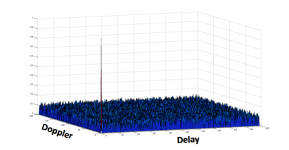
We say that a norm-one sequence is -pseudo-random, —see Figure 1 for illustration—if for every we have
| (II-B.1) |
There are several constructions of families of pseudo-random (PR) sequences in the literature—see [2, 3] and references therein.
II-C Pseudo-Random (PR) Method
Consider a pseudo-random sequence , and assume for simplicity that in (II-B.1). Then we have
| (II-C.1) | |||||
| (II-C.4) |
where are certain multiples of the ’s by complex numbers of absolute value less or equal to one. In particular, we can compute the time-frequency parameter if the associated attenuation coefficient is sufficiently large, i.e., it appears as a “peak” of
Definition II-C.1 (-peak)
Let . We say that at the ambiguity function of and has -peak, if
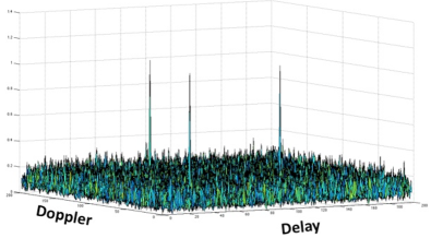
Below we describe—see Figure 2—the PR method.
Pseudo-Random Method
- Input:
-
Pseudo-random sequence , the echo , and a parameter .
- Output:
-
Channel parameters.
Compute on and return those time-frequency shifts at which the -peaks occur.
We call the above computational scheme the PR method with parameter .
Notice that the arithmetic complexity of the PR method is using Remark II-A.1.
III Performance of the PR Method
First, we introduce two important quantities that measure the performance of a detection scheme. These are the probability of detection and the expected number of false targets. Then, we formulate the main result of this note which provides a quantitative statement about the performance of the PR method.
Assume that we have targets out of the possible—see Section I-A. Also, assume that some random data is associated with these targets and influencing the performance of a detection scheme. For example, in our setting the random data consists of (i) the attenuation coefficients associated with the targets, and (ii) the noise. In general, we model the randomness of the data by associating a probability space to the set of targets. For every in the space we denote by and , the number of true and false targets detected by the scheme, respectively. We define the probability of detection by
and the expected number of false targets by
The main result of this note is the following:
Theorem III-.1 (Performance of PR method)
Assume the channel operator (I-A.2) satisfies the uniformity, square root cancellation, and independence assumptions. Then for , where , we have , and , as , for the PR method with parameter .
Remark III-.2 (Rate of convergence)
We suspect that the true rate of convergence in , and , as , is polynomial. In fact, our proof of Theorem III-.1 confirms that the rate of convergence is at least polynomial.
IV Conclusions
The obtained estimates in Theorem III-.1 show that the PR method is effective in terms of performance of detection, in the regime , for . We would like to note that if , for , then the performance of the PR method deteriorates since the noise influence becomes dominant.
V Proof of Theorem III-.1
Before giving a formal proof, we provide a sketch. To detect the parameters of the channel operator , the PR method evaluates the ambiguity function of , and at :
Let us denote by the -th cross term, and by the -th noise component. Then we have
| (V-.1) |
The parameter is detectable by the PR method if the main term is much larger than the -th cross term , and the noise component . For a random point on the unit sphere , by “concentration” most of its coordinates are of absolute value approximately equal to . Thus, if , the magnitude of most of ’s is greater than . Another instance of the concentration phenomenon guarantees that for most channels, the magnitude of the cross term is smaller than . Finally, the square root cancellation assumption on the noise guarantees that the magnitude of the noise term is much smaller than .
We begin the formal proof of the theorem with auxiliary lemmata. In Section VI we prove these statements.
Lemma V-.1 (Largeness of a slice)
Let be a uniformly chosen point on , and fix . There exists (independent of and ), such that for every we have
Lemma V-.2 (Intersectivity)
Let be events in a probability space , such that , , for some . Then for the event
where
we have
Lemma V-.3 (Almost orthogonality)
Let , and let , , be vectors satisfying
Then for any , there exists , such that for a uniformly chosen random point we have
Proof:
Assume that , for some . Let , where is a ()-pseudo-random sequence in , is a channel of sparsity with uniformly distributed attenuation coefficients given by (I-A.2), and satisfies the square root cancellation assumption. We denote , and assume that at the receiver we perform PR method with parameter .
(A) Proof of “ as ”.
We consider two cases.
Case 1. .
Denote by for . Since by Lemma V-.1 there exists such that we have
Therefore, for sufficiently large , we have
Denote by
By Lemma V-.2 we have
| (V-.2) |
Since , we have . Therefore, by Lemma V-.3, there exists such that
| (V-.3) |
It follows from (II-C.1), (V-.2), (V-.3), the square root cancellation and independence assumptions, that with probability greater or equal than , at least of the channel parameters of are detectable.
The latter implies that for sufficiently large. Therefore we have as .
Case 2. .
By Lemma V-.1, there exists such that
By Cauchy-Schwartz inequality we have for all :
It follows from (II-C.1), square root cancellation assumption on the noise, and the last two inequalities that for sufficiently large , all channel parameters of the operator are detectable with probability greater or equal than . Therefore, for sufficiently large we have
The latter implies that as .
(B) Proof of “ as ”.
Case 1. .
By Lemma V-.3, there exists such that we have
where is the set of all channel parameters of . It follows from (II-C.1), the square root cancellation and independence assumptions, and the last inequality that with probability greater or equal than the PR method will not detect any wrong channel parameters. The latter implies that as .
Case 2. .
By Cauchy-Shwartz inequality we have that for every :
It follows from (II-C.1), the square root cancellation assumption on the noise, and the last inequality that there exists such that for sufficiently large we have
The latter implies that the PR method with parameter satisfies as .
VI Proofs of Lemmata
Proof:
We identify the Borel probability space on invariant under all rotations with the Borel probability space of the real unit sphere invariant under all rotations. Recall that
Without loss of generality, it is enough to prove the statement for . Let . We use the notation for the probability space on invariant under all rotations in . For any , and any dimension , we denote the real sphere of radius in by :
Let . By Fubini’s theorem and using the homogeneity of the Lebesgue measure we get
It is well known that
Therefore, for large enough we have
Finally, the containment together with last inequality imply the statement of the lemma.
Proof:
Denote by , and by , . Then we have
On the other hand, we have
The last inequality implies that
It implies
Proof:
Let . We proceed similarly to the proof of Lemma V-.1. Since
and
we conclude that there exists such that
If , then there exists such that
This implies that there exists such that
By the rotation invariance of the Lebesgue measure on , it follows that there exists such that for any set of directions we have
The latter implies the statement of the lemma.
Acknowledgements. We are grateful to our collaborators A. Sayeed, K. Scheim and O. Schwartz, for many discussions related to the research reported in these notes. Also, we thank anonymous referees for numerous suggestions. And, finally, we are grateful to G. Dasarathy who kindly agreed to present this paper at the conference.
References
- [1] Fish A., Gurevich S., Hadani R., Sayeed A., and Schwartz O., Delay-Doppler Channel Estimation with Almost Linear Complexity. IEEE Transactions on Information Theory, Volume 59, Issue 11, 7632-7644, 2013.
- [2] Golomb, S.W., and Gong G., Signal design for good correlation. For wireless communication, cryptography, and radar. Cambridge University Press, Cambridge (2005).
- [3] Gurevich S., Hadani R., and Sochen N., The finite harmonic oscillator and its applications to sequences, communication and radar . IEEE Transactions on Information Theory, vol. 54, no. 9, September 2008.
- [4] Howard S. D., Calderbank, R., and Moran W., The finite Heisenberg–Weyl groups in radar and communications. EURASIP J. Appl. Signal Process (2006).
- [5] Tse D., and Viswanath P., Fundamentals of Wireless Communication. Cambridge University Press (2005).
- [6] Verdu S., Multiuser Detection, Cambridge University Press (1998).