Identification of redundant and synergetic circuits in triplets of electrophysiological data
Abstract
Objective. Neural systems are comprised of interacting units, and relevant information regarding their function or malfunction can be inferred by analyzing the statistical dependencies between the activity of each unit. Whilst correlations and mutual information are commonly used to characterize these dependencies, our objective here is to extend interactions to triplets of variables to better detect and characterize dynamic information transfer. Approach. Our approach relies on the measure of interaction information (II). The sign of II provides information as to the extent to which the interaction of variables in triplets is redundant (R) or synergetic (S). Three variables are said to be redundant when a third variable, say Z, added to a pair of variables (X,Y), diminishes the information shared between X and Y. Similarly, the interaction in the triplet is said to be synergetic when conditioning on Z enhances the information shared between X and Y with respect to the unconditioned state. Here, based on this approach, we calculated the R and S status for triplets of electrophysiological data recorded from drug-resistant patients with mesial temporal lobe epilepsy in order to study the spatial organization and dynamics of R and S close to the epileptogenic zone (the area responsible for seizure propagation). Main results. In terms of spatial organization, our results show that R matched the epileptogenic zone while S was distributed more in the surrounding area. In relation to dynamics, R made the largest contribution to high frequency bands (14-100Hz), whilst S was expressed more strongly at lower frequencies (1-7Hz). Thus, applying interaction information to such clinical data reveals new aspects of epileptogenic structure in terms of the nature (redundancy vs. synergy) and dynamics (fast vs. slow rhythms) of the interactions. Significance. We expect this methodology, robust and simple, can reveal new aspects beyond pair-interactions in networks of interacting units in other setups with multi-recording data sets (and thus, not necessarily in epilepsy, the pathology we have approached here).
Introduction
The use of information theory to deal with data has become an important means to evaluate the interaction between groups of correlated variables in neuroscience, revealing functional relationships and the underlying circuits capable of processing specific information [1, 2, 3, 4]. In addition to information storage/coding/decoding, information theory can address whether interactions between related variables are mutually redundant or synergetic [5, 6].
In general, synergy (S) occurs if the understanding of one variable helps predict the behaviour of another variable with more precision than the sum of the information provided individually by the two variables. By contrast, redundancy (R) corresponds to situations where the same information is offered by the variables (see also the interpretation of S and R based on causality inference in [7]).
When interaction information (II) [8] is applied to sets of three variables, its sign indicates whether the relationship within the triplet can be considered as R or S. Thus, unlike mutual information, II can be either positive or negative, whereby a positive II identifies R and a negative II S. As an example of the mechanisms that produce both R and S, common-cause structures (such a common-input) lead to R, while S could be produced by combining one XOR gate with two independent random inputs (for instance) [9, 10].
The presence of S is well-known in sociological modelling, where the term suppressors was applied to those variables that increase the predictive validity of other variables after their inclusion in a linear regression equation [11]. Similarly, the interaction between triplets of variables in gene regulatory networks was approached to study how a specific gene modulates the interaction between two other genes [12, 13]. Moreover, when applied to electrophysiological recordings from neural networks in culture, a series expansion approach takes into account terms that are coincident with the II [14]. Here, we use II to study triplet interactions in epilepsy but rather than focusing on the pathology, we aim to highlight here the methodological aspects. In particular, by applying II to human electrocorticography data, we reveal certain aspects of the interactions (not captured by looking solely to pairs of variables) that underpin the epileptogenic zone, the brain network that triggers epileptic seizures.
Methods
Surgery and postsurgical outcome
The selection of the area for resection was made according to current standard practices that are applied to surgery for epilepsy, which involves resecting the cortical area that displays the most excitatory activity electrophysiologically as a proxy of the epileptogenic zone [15].
The clinical outcome was assessed using the Engel Epilepsy Surgery Outcome Scale [16], ranging from I (seizure-free after surgery) to IV (no improvement after surgery). The electrocorticography data studied here correspond to n=3 Engel I patients that had no further seizures after surgery and n=1 Engel III patient for comparison.
Human electrocorticography data
The data analyzed here through the novel II approach has been published previously [17] and correspond to data recorded from drug-resistant patients with temporal lobe epilepsy who underwent surgery at the Epilepsy Unit at “La Princesa” Hospital (Madrid, Spain). After receiving the approval of the Ethics Committee at “La Princesa” Hospital, patients provided their informed consent to be evaluated intraoperatively with a subdural electrode grid (interelectrode distance, 1 cm), having been administered low doses of sevoflurane (0.5%) and remifentanil (0.1 mg/kg/min). While recording, the anaesthesia was stabilized within a bispectral index in the range of 55-60 (adimensional index) [18]. The grid was placed over the lateral temporal cortex, with its border parallel to the sylvian fissure and covering gyri T1-T3, and its position was recorded with a video camera or photographed. The reference electrode was placed on the contralateral ear and in some cases it was moved to the nearby scalp in order to verify there was no contamination of the recording, consistent with previous studies [19]. A presurgical evaluation was carried out according to the protocol used at La Princesa Hospital, as reported previously [20].
From the perspective of signal processing, it is important to emphasize the importance of electrocorticography studies as opposed to those based on scalp electroencephalography. In the former signal quality is much better, with a signal to noise ratio about 21 to 115 times greater, which makes these two modalities quite distinct [21].
Data processing
All of the analyses carried out here were performed retrospectively and thus, tailored lobectomies were not based on the results discussed here. An intraoperative electrocorticography session was recorded for 15-20 min using a 32-channel amplifier (Easy EEG II, Cadwell, USA), preprocessing with a filter with a 0.5-400 Hz bandwidth and with a 50 Hz notch filter, and finally downsampling at 200 Hz. Artefact-free epochs of inter-ictal activity lasting up to 5 min were selected by visual inspection. All post-processing analysis was performed in Matlab (MathWorks Inc., Natick, MA).
Frequency-band analysis
Electrophysiological signals were filtered within different frequency bands using a zero-phase digital filter (figure 3). In particular, we used the filtfilt.m function from Matlab (MathWorks Inc., Natick, MA) to filter the following standard bands for brain electrophysiology: delta (1-4 Hz), theta (4-7 Hz), alpha (7-14 Hz), beta (14-26 Hz), and gamma (26-100 Hz).
Shannon entropy
The Shannon entropy of a random variable (i.e.: its average uncertainty) is defined as
| (1) |
where represents the probability distribution of the state of variable [22, 23]. In this manuscript, variable X is defined by the electrical potential captured by electrode X. The joint entropy is just a generalization to any dimension, i.e., in 2D it becomes and in 3D, we have For a base 2 logarithm (as used here), the entropy is expressed in bits.
Interaction information
II is measured based on the Shannon entropy, allowing us to analyze the interactions between triplets [8]. For any triplet , II is defined as
| (2) |
where is the mutual information between and , which can be defined in terms of the marginal and joint entropies, ie.,
| (3) |
and is the conditional mutual information between and conditioned to . Analogously, can be written as a function of the marginal and joint entropies, i.e.,
| (4) |
for further details see [23]. Thus, using the definition given by Eq. (2), and Eqs. (3) and (4), one can express II as a function of the Shannon entropies, i.e.,
| (5) | |||||
From this equation, one can derive simple but important properties of II (for details see Appendix A).
Note that our definition of II uses an opposite sign to the original form in [8]. Also, it is important to emphasize that when II is equal to zero, II is ill-posed as two different situations can correspond to II = 0, namely that the three variables are either statistically independent of each other or that . Therefore, we will only report situations satisfying that II, i.e., values of II will be ignored.
Calculation of the interaction information assuming Gaussian data
We calculated the II under a Gaussian approximation for which the Shannon entropy can be analytically calculated, i.e.: where the differential entropy for the multivariate Gaussian distribution has an analytical derivation (see details in [23]). To calculate the conditional mutual information, Eq. (4), we made use of [24], where for multivariate Gaussian random variables it was shown that:
| (6) |
where denotes the determinant, and the partial covariance matrix is defined by
| (7) |
in terms of the covariance matrix and the cross covariance matrix ; the definition of is analogous, where means appending the two variables.
Calculation of the interaction information assuming non-Gaussian data
In the most general situation of data not following a Gaussian distribution, and in order to calculate the mutual information and the conditional mutual information (cf. rhs in Eq. (2), we first binned the data to 4 states and then evaluated equations (3) and (4) using the Mutual Information Toolbox [25], a C++ implementation of several Information Theory based functions plugged in Matlab (MathWorks Inc., Natick, MA). In particular, we made use of the functions mutualinfo.m and condmutualinfo.m incorporated in [25]. To calculate probabilities, also 6 and 10 bins were used and the results were no different.
Redundancy and synergy
Directly from the definition of II, Eq. (2), a positive sign of II means that , and together with the circulation property (establishing that II is invariant to any possible permutation in ; for further details see Appendix A) this implies that the interaction in the triplet is redundant. Similarly, a negative sign of II corresponds to a synergetic interaction.
This is in agreement with the results based on the partial information decomposition reported in [26], where a similar interpretation of the sign of II was provided: a positive one for R and a negative one for S, taking into account the fact that the right hand side of Eq. (2) has the opposite sign to the II reported in [26] (see also a further discussion in [27]).
Statistical significance
All values reported in this manuscript were statistical significant. Statistical significance was approached by building the null-distribution of no interaction after a shuffling procedure of N=50000 repetitions in the time series used for calculation. Significant values (after Bonferroni correction) were obtained with a p-value of 0.05 for both the S and R tails of the distribution (negative and positive values), as II is not normally distributed, i.e., the tail of the II distribution has a different length on the positive and negative sides.
Averaging of the interaction information
For each of the 20 grid electrodes, we used different non-overlapping windows, ranging from 9 to 29 windows, each containing 2,000 time points (10 seconds at a sampling rate of 200 Hz). The values of II reported here correspond to the average II over all the different windows, producing an appropriate sample (figure S1).
Network measures for plotting interaction information in 2D
To obtain 2D plots of II, whereby each default value depends on a triplet of variables, we represented the II variation across two variables while keeping a third variable fixed.
In order to study the network of interactions rather than looking to individual values, we considered each variable to be a node within a network and after applied different network measures using the Brain Connectivity Toolbox [28, 29]. In particular, the fixed electrode was chosen as the one with maximum betweenness centrality (accounting for the fraction of all the shortest paths in the network that contain a given node, and thus, nodes with high betweenness participate in many of the shortest paths), that with maximum degree (the hub, obtained simply by summing the weighted links connected to a given node), and the one with a maximum clustering coefficient (calculated as the fraction of triangles around a node, and thus providing relevant information of the clustering strength in a node neighbourhood).
Local synchronization index, individual redundancy and individual synergy
In the light of previous studies based on the local synchronization index (LSI) in electrocorticography data [17], we were interested in indexes that can work for individual electrodes. As reported in [17], the LSI measures the average synchronization of each electrode with their first neighbours, including those in the diagonals. In particular, LSI is calculated by averaging the absolute value of the Pearson correlation between a given node and its nearest neighbours, i.e., 3 neighbours at corner’s grid, 5 neighbours at side’s grid and 8 neighbours elsewhere.
In an analogous manner, the individual R was calculated for a given electrode , summing all the values of positive for all and variables. Likewise, the individual S was obtained by summing for all and the negative values of and finally taking the absolute value of this sum. For these two measures, the individual R and S values, we only summed on triplets such that the three variables were distinct to one another.
Results
II depends on triplets of variables and its positivity or negativity identifies rather the interaction in the triplet is (respectively) redundant or synergetic. First, we inspected the patterns of II by projecting it to the 2D plots, fixing one of the electrodes and plotting II by varying the other two variables (see Methods).
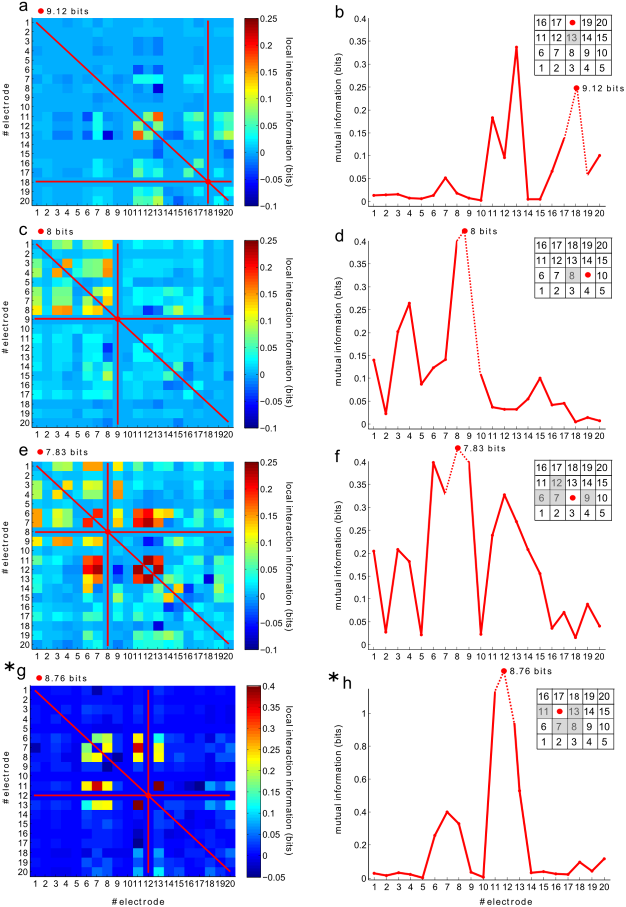
We first fixed the electrodes with maximum and minimum entropy, two good references for studying II as II(X,X,X) coincides with the entropy (see Appendix A). We also fixed several electrodes that at the network level play an important role such as the one with maximum betweenness, the one with maximum degree of connectivity (i.e.: the hub) and the one with a maximum clustering coefficient (see Methods for further details on these measures). As it is shown in figure 1, the 2D plots drastically depend on what the electrode was fixed, indicating a clear 3D structure of II, i.e., a very distinct II patterns appears in the neighbourhood of the different electrodes.
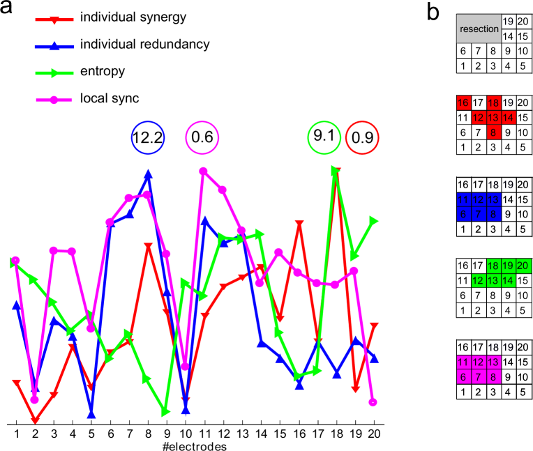
Next, we assessed whether the R and S patterns were in any way related with the epileptogenic zone (the area responsible for seizure propagation). This could be addressed as some of the patients had an Engel I outcome (Methods) and did not experience further seizures after surgery. Given the resection area (an area known for all patients) and using the recordings before surgery, it is possible to guarantee that the resection area contained at least part of the epileptogenic zone. In addition to the resection area (the gray grid in figure 2), we also calculated the spatial distribution of S (red grid in figure 2), R (blue grid), Shannon entropy (green grid) and LSI (the magenta grid), an index that was proven to match the putative epileptogenic zone [17]. Accordingly, while R and LSI had the same spatial grid distribution, the organization of S surrounded them, an observation that was even clearer when II was calculated under the assumption of non-Gaussian data (figure 6). The pattern described by the Shannon entropy was more dispersed, and thus, less related to the epileptic zone.
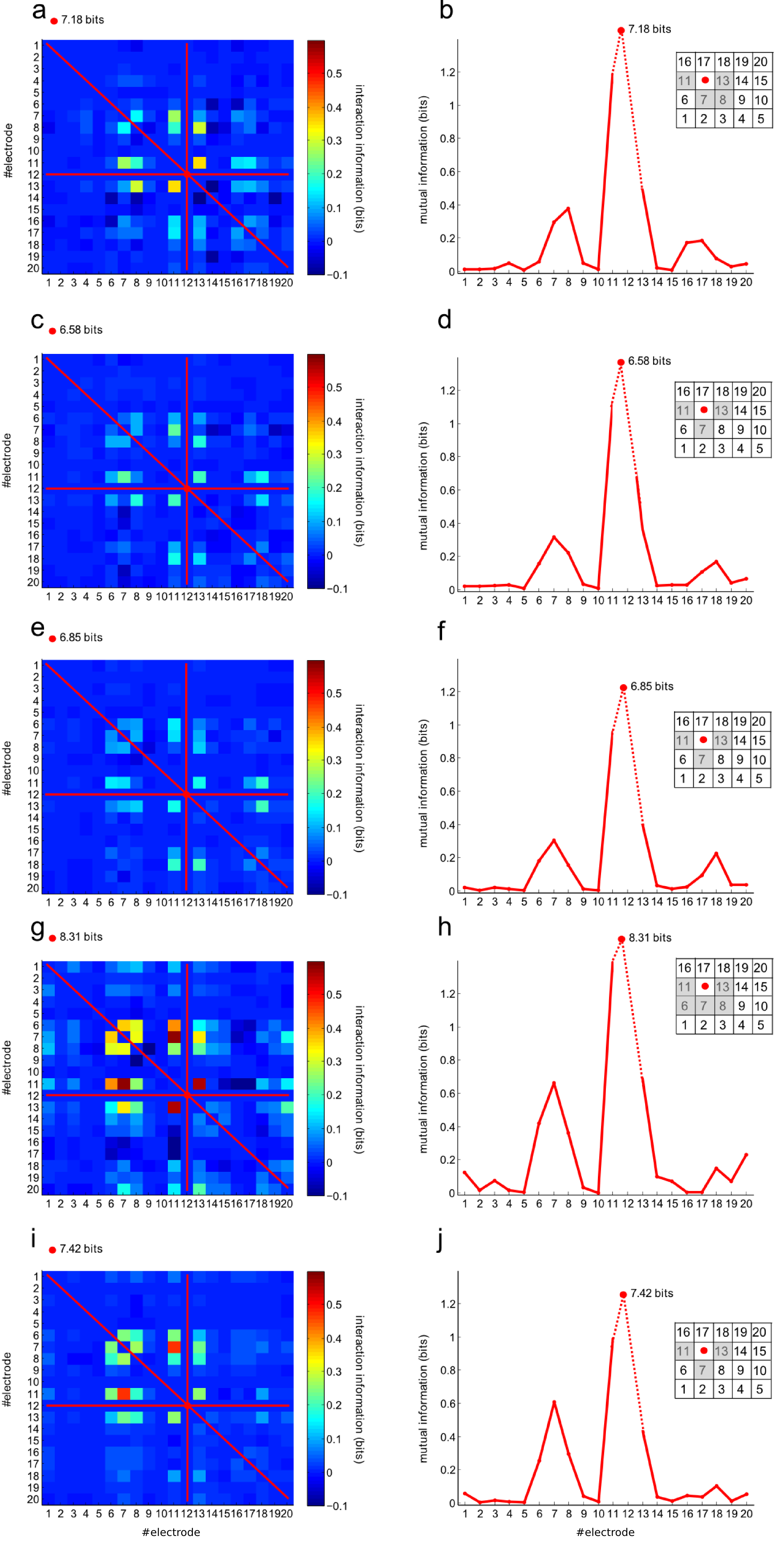
Next, we asked whether the relationship between S/R and LSI (a proxy of the epileptogenic zone) preserved across different brain rhythms. Figure 3 shows 2D plots of II across different frequency bands, keeping fixed one of the electrodes corresponding to the resection area. From top to bottom in figure 3, the lower the panel, the fastest the rhythm was. Thus, straightforward from figure 3, II increased for faster rhythms – beta (14-26 Hz) and gamma (26-100 Hz) bands, the two lowest panels – in comparison to slower ones.
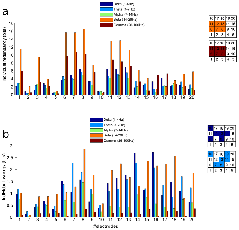
Regarding R and S across frequency bands (figure 4), R had a stronger contribution to high-frequency beta and gamma bands (in orange and brown), while both bands showed a similar spatial distribution, coincident with the LSI that is known to match the epileptogenic zone. By contrast, the low delta and theta bands had a stronger contribution to S (dark and light blues). Importantly, the spatial distribution of S differed considerably from that of R, and while the activation of R matched the epileptogenic zone (i.e., LSI) at high frequencies, S surrounded it and contributed more at low frequency bands.
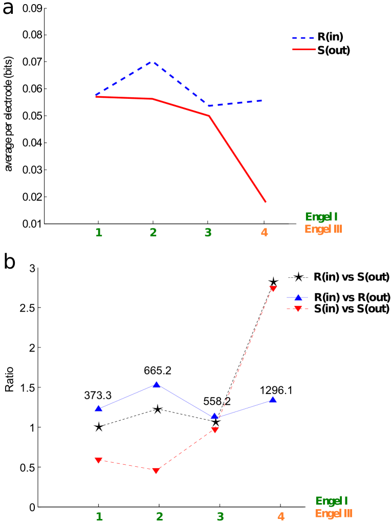
In terms of the robustness of our conclusions across subjects, figures 1-4 are data from one of the patients with Engel I, but similar results were observed for the other patients with the same Engel I outcome. Indeed, figure 5 shows the total amount of R inside the resection area and the total S outside the resection area. For Engel I patients, where the resection area was accurate and patients suffered no further crises, the patterns identified were robust, unlike those from the Engel III patient. This is better captured when the ratio of these quantities is considered, with R within the resection area and S organized across areas surrounding it (see figure 5). In addition, the total R of the Engel III patient is much higher than that of the other three Engel I patients.
Discussion
Studying the interactions among variables in triplets, such as that captured by II, goes beyond bivariate and multivariate studies of interacting variables. Although this method has previously been applied to other fields, to the best of our knowledge we are unaware of similar studies in epilepsy. We have continued earlier studies that took advantage of Granger causality [30] to assess the effects of S and R on epileptic data [31, 32, 7], and we calculated the II in electrocorticography data from epileptic patients who underwent surgery. In particular, we paid special attention to the data from patients that achieved the best possible outcome following surgery and who experienced no further seizures (Engel I patients). Indeed, by taking the resection area in these patients as a reference, we addressed the patterns of II near to the epileptogenic zone, the area essential for seizures to propagate.
We calculated the II in two situations, assuming that the data adopts either a Gaussian or a non-Gaussian distribution. While the former permits an analytical derivation of the II, the non-Gaussian distribution is more general and it is not easy to choose the most appropriate method to estimate probabilities. We are aware that we have applied the simplest method to generate histograms (binning and counting frequencies), as the number of data points was considered to be sufficiently large to guarantee an appropriate sample [33]. Nevertheless, other methods could also be used to estimate probability density, such as kernel estimators, the nearest neighbour method, orthogonal series estimators, etc. (see [34] for further details).
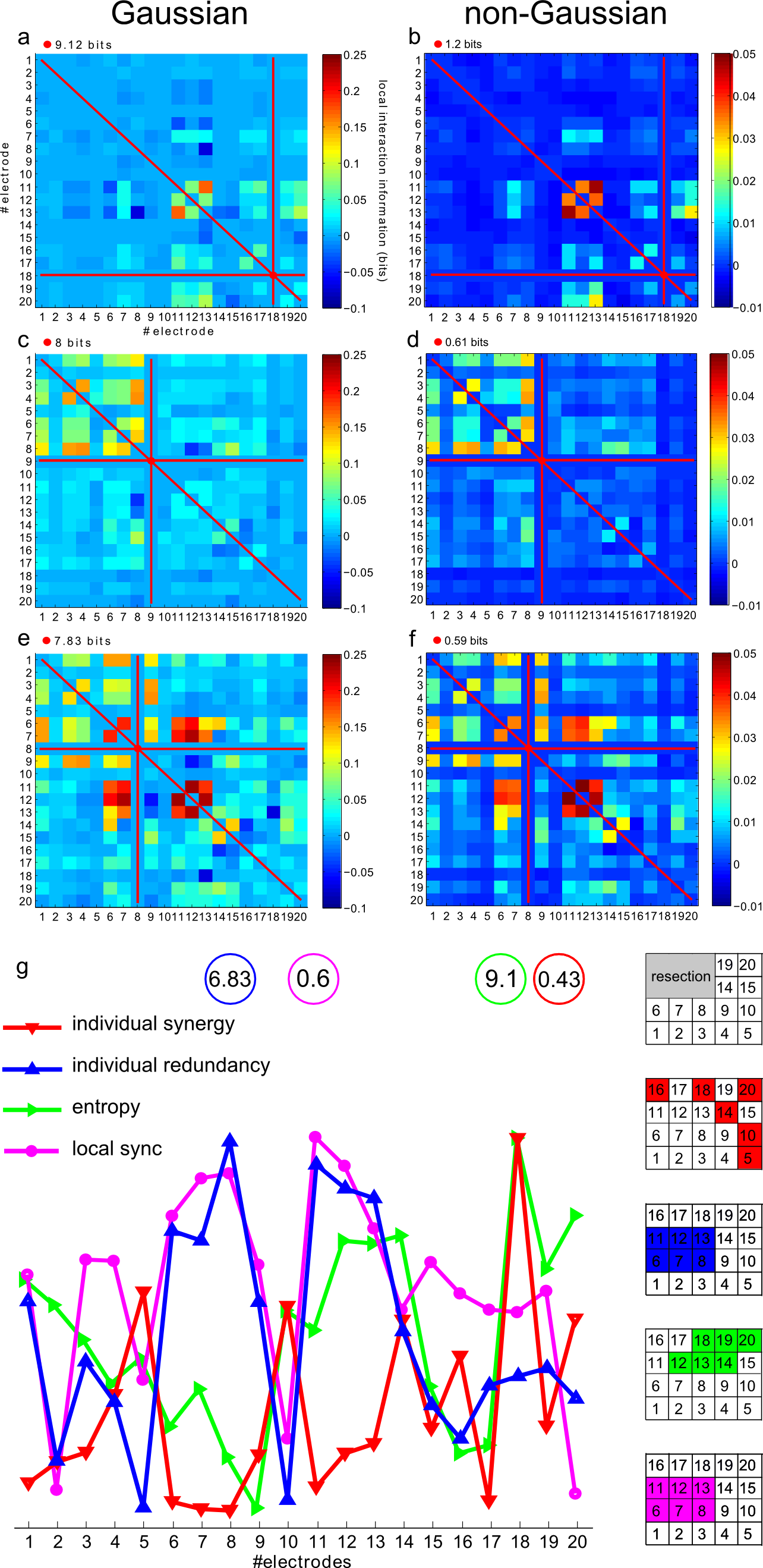
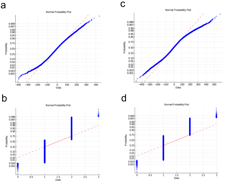
Nevertheless, by assuming Gaussian and non-Gaussian distributions we obtained qualitatively similar results. That is, although data are non-Gaussian across segments, electrodes and patients (figure S3, in addition of obtaining p values of zero after a Kolmogorov-Smirnov for normality test), the Gaussian assumption captures the non-Gaussian character of II quite well. Indeed, although some differences were found with respect to S, the same pattern was observed for R. Importantly, the non-Gaussian assumption was consistent with the Gaussian one in situating S outside the R area.
It is important to emphasize that our aim was to provide a more complete characterization of the informational pattern in the neighbourhood of the epileptogenic zone. Accordingly, the LSI has already been shown to satisfactorily localize the epileptogenic zone [17]. What we found here was that R matched the LSI while S was evident in its surroundings for patients with Engel I. This pattern was particularly clear for II when assuming a non-Gaussian distribution, which is in accordance with the organization of local intracortical interactions that, under the influence of local inhibitory circuits, are responsible for controlling runway excitation [19]. The matching between LSI and R was less clear for a patient with Engel III (figure S2).
Finally, we studied II (including S and R) in relation to interictal activity. However, recent results suggest it might be of interest to carry out further studies into the application of II to pre- and post-ictal activity [35], thereby assessing how the structure of R and S changes with ongoing seizure dynamics.
Acknowledgments
The authors acknowledges Prof. Dante R. Chialvo for having introduced Guillermo J. Ortega to the Computational Neuroimaging Group at Biocruces, making this collaboration possible. We also acknowledge financial support from Ikerbasque: The Basque Foundation for Science, Gobierno Vasco (Saiotek SAIO13-PE13BF001), Junta de Andalucia (P09-FQM-4682) and Euskampus at UPV/EHU to JMC; Ikerbasque Visiting Professor at Biocruces and project “BRAhMS – Brain Aura Mathematical Simulation” (AYD-000-285), co-funded by Bizkaia Talent and European Commission through COFUND programme to SS; pre-doctoral contract from the Basque Government, Eusko Jaurlaritza, grant PRE/2014/1/252, to AE.
References
References
- [1] Borst A and Theunissen F 1999 Nat. Neurosci. 2 947–967
- [2] Panzeri S, Schultz S, Treves A and Rolls E 1999 Proc. Bio.l Sci. 266 1001–1012
- [3] Quiroga R and Panzeri S 2009 Nat. Rev. Neurosci. 10 173–185
- [4] Cortes J, Marinazzo D and Munoz M 2014 Front. Neuroinform. 8 86
- [5] Schneidman E, Bialek W and Berry M 2003 J. Neurosci. 23 11539–11553
- [6] Bettencourt L, Stephens G, Ham M and Gross G 2007 Phys. Rev. E 75 021915
- [7] Stramaglia S, Cortes J and Marinazzo D 2014 New J. Phys. 16 105003
- [8] McGill W 1954 Psychometrika 19 97–116
- [9] Lizier T, Atay F and Jost J 2012 Phys Rev E 86 026110
- [10] Wibral M, Lizier J, Voegler S, Priesemann V and Galuske R 2014 Front. Neuroinform. 8 1
- [11] Conger A 1974 Educational and Psychological Measurement 34 35–46
- [12] Antonov A, Tetko I, Mader M, Budczies J and Mewes H 2004 Bioinformatics 20 644–652
- [13] Wang K, Saito M, Bisikirska B, Alvarez M, Lim W, Rajbhandari P, Shen Q, Nemenman L, Basso I, Margolin A, Klein U, Dalla-Favera R and Califano A 2009 Nat. Biotechnol. 27 829–839
- [14] Bettencourt L, Gintautas V and Ham M 2008 Phys. Rev. Lett. 100 238701
- [15] Rosenow F and Luders H 2001 Brain 124 1683–1700
- [16] Engel J, Ness P V, Rasmussen T and Ojemann L 1993 Surgical Treatment of the Epilepsies (New York: Raven Press) chap Outcome with respect to epileptic seizures
- [17] Palmigiano A, Pastor J, de Sola R G and Ortega G 2012 PLoS One 7 e41799
- [18] Rosow C and Manberg P 2001 Anesthesiol. Clin. North America 19 947–966
- [19] Ortega G, de la Prida L M, de Sola R G and Pastor J 2008 Epilepsia 49 269–280
- [20] Pastor J, Hernando-Requejo V, Dominguez-Gadea L, de Llano I, Meilan-Paz M, Martinez-Chacon J and de Sola R G 2005 Revista Neurologia 41 709–716
- [21] Ball T, Kerna M, Mutschler I, Aertsen A and Schulze-Bonhage A 2009 Neuroimage 46 708–716
- [22] Jaynes E 1957 Phys. Rev. 106 106 620–630
- [23] Cover T and Thomas J 2006 Elements of Information Theory (John Wiley & Sons, Inc)
- [24] Barnett L, Barrett A and Seth A 2009 Phys. Rev. Lett. 103 238701
- [25] Peng H, Long F and Ding C 2005 IEEE Trans. Pattern Anal. Mach. Intell. 27 1226–1238
- [26] Williams P L and Beer R D 2010 arXiv preprint arXiv:1004.2515
- [27] Barrett A 2015 Phys. Rev. E 91 052802
- [28] Rubinov M and Sporns O 2010 Neuroimage 52 1059–1069
- [29] Brain Connectivity Toolbox https://sites.google.com/site/bctnet/
- [30] Granger C 1969 Econometrica 37 424–438
- [31] Marinazzo D, Liao W, Pellicoro M and Stramaglia S 2010 Phys. Lett. A 374 4040–4044
- [32] Wu G, Chen F, Kang D, Zhang X, Marinazzo D and HChen 2011 IEEE Trans. Biomed. Eng. 58 3088–3096
- [33] Bonachela J, Hinrichsen H and Munoz M 2008 J. Phys. A 41 202001
- [34] Bishop C 2006 Pattern recognition and machine learning (Springer)
- [35] van Mierlo P, Papadopoulou M, Carrette C, Boon P, Vandenberghe S, Vonck K and Marinazzo D 2014 Prog. Neurobiol. 121 19–35
Appendix A: Properties satisfied by the interaction information
Directly from equation (5), one can derive important properties which are particularly relevant to the present work:
-
•
Circulation: II is invariant to any possible permutation in and thus, the evaluation of II gives the same result for each of the following six situations , , , , , . The proof is straightforward just using the Eq. (5).
-
•
Mutual information limit: in the case of triplets with only 2 distinct variables, i.e.: , , , is satisfied, thus, II is equal to the mutual information between the two distinct variables. The proof of this is straightforward as, by definition, the entropy satisfies that and that . Thus, the definition of the mutual information given in Eq. (3) provides the proof.
-
•
Shannon entropy limit: in the case of triplets with three equal variables, the equality of II holds, i.e.: II is equal to the Shannon entropy of the variable. The proof of this is straightforward and is similar to the one derived for the mutual information limit.
Figure Legends
Figure 1: Structure of the interaction information in epilepsy based on human electrocorticography data. Positive values of II indicate R, whereas negative values indicate S. The 2D plots of II were obtained by varying two variables but keeping one of them fixed. In particular, we fixed the electrode with a: maximum entropy ( that for this particular case was coincident with the electrode with maximum betweenness) c: minimum entropy e: maximum degree (the hub, for this particular case was coincident with the electrode with maximum clustering coefficient). g: electrode number 12, as a representative belonging to the resection area. a,c,e,g: red lines correspond to the mutual information between the electrode that was kept fixed and the rest of electrodes in the grid. Indeed, as shown in Appendix A, II is coincident with the mutual information when two variables are equivalent in the triplet. The solid red circle is the Shannon entropy value of the electrode that was fixed (coincident with II(X,X,X)). b,d,f,h: Same red lines as in panels a, c, e, g. Dashed lines have been introduced to show when the Shannon entropy value is much bigger than the values of mutual information. Electrocorticography grids are also plotted to show that similar values of mutual information were clustered within a geometrical similar region of the grid (in gray we plot the values of mutual information larger than 0.3 bits). Note that while II can be either positive or negative, the mutual information is strictly positive (when it is zero, statistical independence is indicated). g,h: (*) Different scale.
Figure 2: Synergetic and redundant interactions in epilepsy from human electrocorticography data. a: Varying (as explained in the methods), we can sum all the negative values of to obtain the individual S (red) and similarly, the positive values of to achieve the individual R (blue). In green, we plot the Shannon entropy for each electrode (i.e.: , see Appendix A for further details) and in magenta, the LSI as measured in [17], summing the absolute value of the correlations between each electrode and its neighbouring electrodes in the grid. Note that for illustrative purposes the four measures are represented in an arbitrary scale. We plotted the maximum values for each measure in coloured circles. b: The six maximum electrode values for each of the measures plotted in panel a. In addition, we also plotted the resection area in gray, in this case from a patient in which the seizures disappeared after surgery.
Figure 3: Structure of the interaction information in epilepsy at different frequency-bands obtained from human electrocorticography data. As in figure 1, we plot II keeping one electrode belonging to the resection area fixed across the different frequency bands: a,b delta (1-4 Hz) c,d theta (4-7 Hz) e,f alpha (7-14 Hz) g,h beta (14-26 Hz) and i,j gamma (26-100 Hz). One can see how the values of II are higher at and bands. b,d,f,h,j: Similar to figure 1, we plot in gray the values of mutual information larger than 0.3 bits.
Figure 4: Redundancy and synergy across frequency bands. a: R receives a larger contribution from the high-frequency beta and gamma bands (orange and brown), with both bands showing a similar spatial grid map overlapping with the epileptogenic zone (cf. figure 2). b: The low delta and theta made a stronger contribution to S (dark and light blue). Importantly, the spatial distribution of S is quite different from that of R: whilst the activation of R overlaps the epileptogenic zone and it is represented by high frequencies, S tends to surround this region and it operates in low frequency bands.
Figure 5: Validation across patients. a: We plotted the average values of R for each electrode inside the resection area (blue dashed line) and S outside the resection area (red solid line) – the total amount of R inside and S outside divided by the number electrodes in the resection area –. This was done for 3 patients with Engel I (where the resection area matched or exceeded the epileptogenic zone) and for 1 patient with Engel III (to illustrate at least one case where the resection area did not match the epileptogenic zone). The Engel I and III patterns were quite different. b: The ratio between R inside the resection area –R(in)– divided by that of S outside that area –S(out)–, and both the ratios of S inside –S(in)– divided by S(out) or R(in) divided by R(out). There are clearly important differences between Engel I and Engel III patients, corroborating the dynamic pattern found: R within the epileptogenic zone and S organized in the surrounding region. The total R for each patient is also represented (i.e., numbers 373.3, 665.2, 558.2 and 1296.1) whereby the Engel III value is much larger than that for the Engel I cases.
Figure 6: Comparison between the Gaussian and the non-Gaussian assumptions. Panels a, c and e have been plotted again from figure 1 for ready comparison. The interaction information obtained when keeping the electrode fixed with: a,b: maximum entropy; c,d: minimum entropy e,f: maximum degree (the hub that in this particular situation is coincident with the electrode with the highest clustering coefficient). b, d, f: The scenario for non-Gaussian data does not change qualitatively with respect to the Gaussian assumption. g: As in figure 2 but assuming a non-Gaussian distribution. Note that the same pattern is observed for R whilst some differences are found for S. Now, the statement of R and LSI having a similar spatial grid, and S surrounding R, is more clear than for the Gaussian case.
Legends to Supporting Information
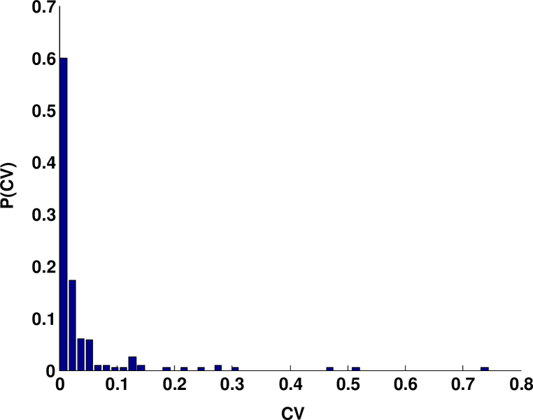
Figure S1: Sampling validation of the interaction information. The figure shows the coefficient of variation of the II (standard deviation of the estimation divided by its mean) resulting from averaging over 9 different windows and consisting of 2000 points each. One can see how the standard deviation is well-sampled and significantly smaller than the average.
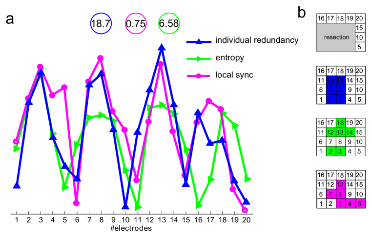
Figure S2: Redundant interactions in epilepsy from human electrocorticography data for a patient with Engel III. Similar to figure 2 but for a patient with Engel III, i.e., with patient’s seizures not disappearing after surgery. Observe that the three electrodes 3, 8 and 13 have maximum LSI (local sync, an index which was proven to match the epileptogenic zone in [17]) and also have maximum R.
Figure S3: Evidence of non-Gaussianity in the data. Normal probability plots indicate strong data deviation from Gaussianity (the more the data do not follow the straight line, the more non-Gaussian is). a: data corresponding to one subject, one electrode and one of the segments used to average and calculate II (and therefore, R and S). b: Same data that in a, but binned to 4 states. Non-gaussianity also applied to binned data. c,d: Similar to panels a and b, for the same subject but different electrode. The same results are valid across subjects.
