Pinning dynamic systems of networks with Markovian switching couplings and controller-node set

Yujuan Han 09210180039@fudan.edu.cn Wenlian Lu wenlian@fudan.edu.cn Zhe Li 11210180026@fudan.edu.cn Tianping Chen tchen@fuan.edu.cn School of Mathematical Sciences, Fudan University, Shanghai 200433, China Centre for Computational Systems Biology, Fudan University, Shanghai 200433, China Department of Computer Science, The University of Warwick, Coventry CV4 7AL, United Kingdom School of Computer Science, Fudan University, Shanghai 200433, China
Abstract

In this paper, we study pinning control problem of coupled dynamical systems with stochastically switching couplings and stochastically selected controller-node set. Here, the coupling matrices and the controller-node sets change with time, induced by a continuous-time Markovian chain. By constructing Lyapunov functions, we establish tractable sufficient conditions for exponentially stability of the coupled system. Two scenarios are considered here. First, we prove that if each subsystem in the switching system, i.e. with the fixed coupling, can be stabilized by the fixed pinning controller-node set, and in addition, the Markovian switching is sufficiently slow, then the time-varying dynamical system is stabilized. Second, in particular, for the problem of spatial pinning control of network with mobile agents, we conclude that if the system with the average coupling and pinning gains can be stabilized and the switching is sufficiently fast, the time-varying system is stabilized. Two numerical examples are provided to demonstrate the validity of these theoretical results, including a switching dynamical system between several stable sub-systems, and a dynamical system with mobile nodes and spatial pinning control towards the nodes when these nodes are being in a pre-designed region.

keywords:
pinning control; coupled dynamical system; Markovian switching; spatial pinning control
fn1fn1footnotetext: This work is jointly supported by the National Key Basic Research and Development Program (No. 2010CB731403), the National Natural Sciences Foundation of China under Grant Nos. 61273211, 60974015, and 61273309, the Marie Curie International Incoming Fellowship from the European Commission (FP7-PEOPLE-2011-IIF-302421), and also the Laboratory of Mathematics for Nonlinear Science, Fudan University.

1 Introduction

Control and synchronization of large-scale dynamical systems have attracted wide interests over the past decades since the new discoveries of small-world and scale-free features [1, 2]. When the network cannot be stabilized by itself, many control strategies are taken into account to force the network to be stable. Among these control strategies, pinning control is brilliant because it is easily realizable by controlling a partial of the nodes instead of all nodes in the network.

The general idea behind pinning control is to apply some local feedback controllers only to a fraction of nodes and the rest of nodes can be propagated through the coupling among nodes. In most existing papers, authors considered two different pinning strategies: randomly pinning and selective pinning based on the connectivity degrees. [3, 4] concluded that pinning of the most highly connected nodes performance better stabilizability than the randomly pinning scheme. [5]-[7] used Lyapunov functions, master stability functions and algebraic properties of the coupling matrix to study pinning control of complex network. [8]-[12] gave conditions based on the graph topology of the network guaranteeing stability. In these papers, networks with time-invariant links were considered. [13] studied the global pinning synchronization of Lorenz-type dynamical networks with both fixed and switching topologies. It was proved that if each possible network topology contains a directed spanning tree and the dwell time of switching is larger than a positive threshold, global pinning synchronisation in switching networks with a suitable coupling strength can be guaranteed. However, pinning dynamic systems of networks with stochastically switching topologies is absent.

Noting that stability and controllability of stochastic differential equations have been well studied these years [14]-[17], in which differential dynamical systems with Markovian switching have received lots of research interests [18]-[20]. In these papers, the stability of linear, semi-linear and nonlinear equations with Markovian switching were studied and some sufficient criteria were established based on Lyapunov functions and linear matrix inequalities. Hence, in this paper, we investigate the pinning control of networks with Markovian switching topologies.

However, for a network of mobile agents, it is difficult to implement a pinning control strategy because the selected controllers are moving. [22]-[24] investigated the flocking control via selecting some fixed nodes to be pinned prior. To avoid this, [25] introduced the concept of spatial pinning control for network via applying controllers only on nodes (agents) which enter a given area, called control region. In its setup, agents move following random walking in a planar space and interact according to a time-varying $r$-disk proximity graph. In the this paper, we considered a more general case, the moving motion of each agent follows a Markov process.

Inspired by these works, we investigate the pinning control of a complex network with Markovian switching couplings to an arbitrary trajectory of the uncoupled node system by Markovian selected controller-node set. We derive analytical conditions for the stability of the system at the homogeneous trajectory. Based on the switching speed of the couplings and controller-node sets, two scenarios are considered here. Firstly, if each subsystem in the switching system with fixed couplings can be stabilized by fixed pinning nodes and the Markovian switching is sufficiently slow, the system can be stabilized. Secondly, if the system with average coupling matrix and pinning gains can be stabilized and the Markovian switching is sufficiently fast, the system can be stabilized. As an application, we also study the spatial pinning control problem of network with mobile agents.

This paper is organized as follows. Section 2 presents some definitions and some notations required in this paper. Section 3 investigates the pinning control problem of network with Markovian switching coupling. Section 4 investigates the fast switching networks and as an application, the spatial pinning control of network of mobile agents is considered. Simulations are given in section 5 to verify the theoretical results. Finally, conclusions are drawn in section 6.

2 Preliminaries

At first, we introduce some notations needed throughout this paper. For a matrix $A$, denote $a_{ij}$ the elements of $A$ on the $i$th row and $j$th column. $A^{\top}$ denotes the transpose of $A$. $A^{s}=(A+A^{\top})/2$ denotes the symmetry part of a square matrix $A$. Denote by $A>0(\geq 0)$ that $A$ is a positive(semi-positive) definite and so is with $<0$ and $\leq 0$. $I_{m}$ denotes the identity matrix with dimension $m$. For a symmetric square matrix $A$, denote $\lambda_{M}(A)$ and $\lambda_{m}(A)$ the largest and smallest eigenvalues of $A$ respectively, $\lambda_{i}(A)$ the i-th largest eigenvalue of $A$. $\|z\|$ denotes a vector norm of a vector $z$, $\|A\|$ denotes the matrix norm of $A$ induced by the vector norm $\|\cdot\|$ and denote $\|A\|_{\infty}=\max_{i,j}|a_{ij}|$. In particular, without special notes, $\|z\|=\|z\|_{2}=\sqrt{\sum_{i}|z_{i}|^{2}}$, the $2$-norm. The symbol $\otimes$ is the Kronecker product.

Linearly coupled ordinary differential equations (LCODEs) are used to describe coupling dynamical systems, which can be described as follows:

xΛ™i=f​(xi,t)+ΞΊβ€‹βˆ‘j=1,jβ‰ imli​j​(t)​Γ​[xj​(t)βˆ’xi​(t)],superscriptΛ™π‘₯𝑖𝑓superscriptπ‘₯π‘–π‘‘πœ…superscriptsubscriptformulae-sequence𝑗1π‘—π‘–π‘šsubscript𝑙𝑖𝑗𝑑Γdelimited-[]superscriptπ‘₯𝑗𝑑superscriptπ‘₯𝑖𝑑\displaystyle\dot{x}^{i}=f(x^{i},t)+\kappa\sum_{j=1,j\neq i}^{m}l_{ij}(t)\Gamma[x^{j}(t)-x^{i}(t)],
$\displaystyle~{}i=1,\cdots,m.$ (1)

where $x^{i}(t)=[x^{i}_{1}(t),\cdots,x^{i}_{n}(t)]\in\mathbb{R}^{n}$ is the state variable of the $i$th node, $t\in[0,+\infty)$ is the continuous time, $f$: $\mathbb{R}^{n}\times\mathbb{R}^{+}\mapsto\mathbb{R}^{n}$ is the dynamics of the uncoupled nodes, $\kappa$ is the coupling strength, $l_{ij}(t)$ denotes the coupling coefficient from agent $j$ to agent $i$ at time $t$, $\Gamma=[\gamma_{kl}]_{k,l=1}^{n}\in\mathbb{R}^{n\times n}$ denotes the inner connection matrix with Ξ³k​lβ‰ 0subscriptπ›Ύπ‘˜π‘™0\gamma_{kl}\neq 0 if two agents are connected by their $k$th and $l$th state component respectively. For iβ‰ j𝑖𝑗i\neq j, let li​i​(t)=βˆ’βˆ‘j=1,jβ‰ inli​j​(t)subscript𝑙𝑖𝑖𝑑superscriptsubscriptformulae-sequence𝑗1𝑗𝑖𝑛subscript𝑙𝑖𝑗𝑑l_{ii}(t)=-\sum_{j=1,j\neq i}^{n}l_{ij}(t), then the coupling matrix $L(t)=[l_{ij}(t)]$ is a Metzler matrix with zero row sums at time $t$.

Suppose $\sigma_{t}$ is a homogeneous continuous Markov chain with a finite state space $\mathbb{S}=\{1,2,\cdots,N\}$ and its generator $Q=[q_{ij}]_{N\times N}$ is given by

ℙ​{Οƒt+Ξ”=j|Οƒt=i}={qi​j​Δ+o​(Ξ”),iβ‰ j,1+qi​i​Δ+o​(Ξ”),i=j,β„™conditional-setsubscriptπœŽπ‘‘Ξ”π‘—subscriptπœŽπ‘‘π‘–casessubscriptπ‘žπ‘–π‘—Ξ”π‘œΞ”π‘–π‘—1subscriptπ‘žπ‘–π‘–Ξ”π‘œΞ”π‘–π‘—\displaystyle\mathbb{P}\{\sigma_{t+\Delta}=j|\sigma_{t}=i\}=\left\{\begin{array}[]{lr}q_{ij}\Delta+o(\Delta),&i\neq j,\\ 1+q_{ii}\Delta+o(\Delta),&i=j,\end{array}\right.

where $\Delta>0$, $\lim_{\Delta\to 0}(o(\Delta)/\Delta)=0$, $p_{ij}=-\frac{q_{ij}}{q_{ii}}>0$ is the transition probability from $i$ to $j$ if jβ‰ i𝑗𝑖j\neq i, while qi​i=βˆ’βˆ‘j=1,jβ‰ iNqi​jsubscriptπ‘žπ‘–π‘–superscriptsubscriptformulae-sequence𝑗1𝑗𝑖𝑁subscriptπ‘žπ‘–π‘—q_{ii}=-\sum_{j=1,j\neq i}^{N}q_{ij}.

Denote $P=[p_{ij}]$ the transition matrix of this Markov process. Let $\Delta_{k},k=0,1,\cdots$ be the successive sojourn time between jumps. The sojourn time in state $i$ is exponentially distributed with parameter $q_{i}$.

Denote $\pi(k)=[\pi_{1}(k),\cdots,\pi_{N}(k)]$ the state distribution of the process at the $k-$th switching. From the Chapman-Kolmogorov equation [29], the $k-$th time distribution can be expressed in terms of the initial state distribution and the transition matrix, that is $\pi(k)=\pi(0)P^{k}$. Suppose the Markov chain $\sigma_{t}$ is ergodic, then from [30], we have that $P$ is a primitive matrix and there exists a state distribution $\bar{\pi}=[\bar{\pi}_{1},\cdots,\bar{\pi}_{N}]$ with positive entries satisfies $\bar{\pi}=\bar{\pi}P$. From [34], we obtain that there exists positive numbers $M$ and $\zeta<1$ such that

$\displaystyle|\pi_{j}(k)-\bar{\pi}_{j}|<M\zeta^{k}.$ (3)

Pick $\pi_{j}=\frac{\bar{\pi}_{j}/q_{j}}{\sum_{i=1}^{N}\bar{\pi}_{i}/q_{i}},j=1,\cdots,N$ and $\pi=[\pi_{1},\cdots,\pi_{N}]$. Then, we have $\pi Q=0$. We call $\pi$ the invariant distribution of Markov process $\sigma_{t}$.

Throughout the paper, we assume $f(x^{i},t)$ belongs to the following function class QUAD $(G,\alpha\Gamma,\beta)$.

Definition 1

Function class QUAD $(G,\alpha\Gamma,\beta)$: let $G$ be an $n\times n$ positive definite matrix and $\Gamma$ be an $n\times n$ matrix. QUAD$(G,\alpha\Gamma,\beta)$ denotes a class of continuous functions $f(\xi,t):\mathbb{R}^{n}\times[0,+\infty)\mapsto\mathbb{R}^{n}$ satisfying

$\displaystyle(\xi-\zeta)^{\top}G[f(\xi,t)-f(\zeta,t)-\alpha\Gamma(\xi-\zeta)]$
$\displaystyle\leq-\beta(\xi-\zeta)^{\top}(\xi-\zeta),$

holds for some $\beta>0$ and all $\xi,\zeta\in\mathbb{R}^{n}$.

We say $f(\cdot,t)$ is globally Lipschitz if $\|f(\xi,t)-f(\zeta,t)\|\leq Lf\|\xi-\zeta\|$ holds for some $Lf>0$ and all $\xi,\zeta\in\mathbb{R}^{n}$.

QUAD condition defines a class of functions arising in stability by quadratic type of Lyapunov function and it is also known as $V$-decreasing in some contexts [8]. It has a strong connection to other function classes, such as Lipschtiz condition and contraction. As mentioned in [9], QUAD condition is weaker than Lipschtiz condition. since any globally Lipschitz continuous function can be QUAD for sufficiently large $\alpha$ and $G=\Gamma=I_{n}$.

In this paper, we consider the pinning controlled network as follows:

$\displaystyle\dot{x}^{i}(t)=f(x^{i}(t),t)+\kappa\sum_{j=1}^{m}l_{ij}(\sigma_{t})\Gamma x^{j}(t)$
+κ​ϡ​ci​(Οƒt)​Γ​(s​(t)βˆ’xi​(t)),i=1,β‹―,m.formulae-sequenceπœ…italic-Ο΅subscript𝑐𝑖subscriptπœŽπ‘‘Ξ“π‘ π‘‘superscriptπ‘₯𝑖𝑑𝑖1β‹―π‘š\displaystyle+\kappa\epsilon c_{i}(\sigma_{t})\Gamma(s(t)-x^{i}(t)),~{}i=1,\cdots,m. (4)

where $\epsilon>0$ is the feedback control gain, $c_{i}(\tau)$ is a variable that takes values $0,1$, $\sigma_{t}$ is a homogeneous Markov chain proposed in section 2, $s(t)$ satisfying $\dot{s}(t)=f(s(t),t)$ is the target trajectory of node dynamics. Here, $s(t)$ may be an equilibrium point, a periodic orbit, or even a chaotic orbit. The initial value $x(0)=x_{0}$ is chosen randomly and independent of the other random variables. Denote $L(\sigma_{t})=[l_{ij}(\sigma_{t})]$ and $C(\sigma_{t})=diag\{c_{1}(\sigma_{t}),\cdots,c_{m}(\sigma_{t})\}$.

We define the pinning control problem as a synchronizing all the states of the nodes in the dynamical network to an arbitrary trajectory $s(t)$ of the uncoupled dynamical system. Therefore, in the following, we study the stability of $s(t)$ in system (4).

Definition 2

System (4) is said to be exponentially stable at $s(t)$ in mean square sense, if there exists constants $\delta>0$ and $M>0$, such that

$\displaystyle\mathbb{E}\bigg{[}\|x^{i}(t)-s(t)\|^{2}\bigg{]}\leq Me^{-\delta t}$ (5)

holds for all $t>0$ and any $i=1,\cdots,m$.

Definition 3

The system (4) is stable almost surely if

$\displaystyle\mathbb{P}\bigg{[}\lim_{t\to+\infty}\|x^{i}(t)-s(t)\|=0\bigg{]}=1$ (6)

holds for all $i=1,\cdots,m$.

3 Pinning time-varying networks

In this section, we suppose $\sigma_{t}$ is with a finite state space $\mathbb{S}=\{1,\cdots,N\}$.

Theorem 1

Suppose $f(x^{i},t)\in QUAD(G,\alpha\Gamma,\beta)$ and there exist diagonal positive definite matrices $P_{i},i=1,\cdots,N$ such that

$\displaystyle\{P_{i}[\alpha I_{m}+\kappa L(i)-\kappa\epsilon C(i)]\otimes G\Gamma\}^{s}$
$\displaystyle+\sum_{j=1}^{m}q_{ij}P_{j}\otimes G\leq 0,~{}\rm{for~{}all}~{}i\in\mathbb{S},$ (7)

then the system (4) is exponentially stable at the homogeneous trajectory in mean square sense.

Proof.Β  Let $x=[{x^{1}}^{\top},\cdots,{x^{m}}^{\top}]^{\top}$,$\hat{s}=[s^{\top},\cdots,s^{\top}]^{\top}$, $y=x-\hat{s}$, $F(x)=[f(x^{1})^{\top},\cdots,f(x^{m})^{\top}]^{\top}$, $C(\sigma_{t})=diag\{c_{1}(\sigma_{t}),\cdots,c_{m}(\sigma_{t})\}$ and ${\tilde{P}}_{\sigma_{t}}=P_{\sigma_{t}}\otimes G$, then we define $V(y,t,\sigma_{t})=\displaystyle\frac{1}{2}y^{\top}{\tilde{P}}_{\sigma_{t}}y$. The joint process $\{(y(t),\sigma_{t}):t>0\}$ is a strong Markov process and the infinitesimal generator of the process is:

$\displaystyle\mathcal{L}=Q+diag\{y^{\top}P^{\top}(1)\frac{\partial}{\partial y},\cdots,y^{\top}P^{\top}(m)\frac{\partial}{\partial y}\}$

Then, we have

$\displaystyle\mathcal{L}V(y,t,i)$ $\displaystyle=$ $\displaystyle\sum_{j=1}^{N}q_{ij}V(y,t,j)+(\frac{\partial V(y,t,i)}{\partial y})^{\top}\dot{y},$ (8)

Let $0<\delta\leq\frac{2\beta\min_{i,j}(P_{j})_{ii}}{\max_{i}\{\lambda_{M}(P_{i})\}}$. From the Dynkin Formula [20], we have

$\displaystyle\mathbb{E}e^{\delta t}V(y,t,\sigma_{t})$
$\displaystyle=$ $\displaystyle V(y_{0},0,\sigma_{0})+\delta\mathbb{E}\int_{0}^{t}e^{\delta\tau}V(y,\tau,\sigma_{\tau})d\tau$
$\displaystyle+\mathbb{E}\int_{0}^{t}e^{\delta\tau}\mathcal{L}V(y,\tau,\sigma_{\tau})d\tau$
$\displaystyle\leq$ $\displaystyle V(y_{0},0,\sigma_{0})+\delta\mathbb{E}\int_{0}^{t}e^{\delta\tau}V(y,\tau,\sigma_{\tau})d\tau$
$\displaystyle-\min_{i,j}(P_{j})_{ii}\mathbb{E}\int_{0}^{t}e^{\delta\tau}\beta y^{\top}yd\tau$
$\displaystyle+\mathbb{E}\int_{0}^{t}e^{\delta\tau}y^{\top}\{P_{\sigma_{\tau}}[\alpha I_{m}+\kappa L(\sigma_{\tau})-\kappa\epsilon C(\sigma_{\tau})]$
$\displaystyle\otimes G\Gamma+\sum_{j=1}^{m}q_{\sigma_{\tau}j}P_{j}\otimes G\}^{s}yd\tau$
$\displaystyle\leq$ $\displaystyle V(y_{0},0,\sigma_{0})+\delta\mathbb{E}\int_{0}^{t}e^{\delta\tau}V(y,\tau,\sigma_{\tau})d\tau$
$\displaystyle-\min_{i,j}(P_{j})_{ii}\mathbb{E}\int_{0}^{t}e^{\delta\tau}\beta y^{\top}yd\tau$
$\displaystyle\leq$ $\displaystyle V(y_{0},0,\sigma_{0})+\mathbb{E}\int_{0}^{t}e^{\delta\tau}[-\min_{i,j}(P_{j})_{ii}\beta$
$\displaystyle+\frac{1}{2}\delta\max_{i}\{{\lambda_{M}({\tilde{P}}_{i})}\}]y^{\top}yd\tau$
$\displaystyle\leq$ $\displaystyle V(y_{0},0,\sigma_{0})$

The first inequality is because of (8), $f(x,t)\in QUAD(G,\alpha\Gamma,\beta)$ and the second inequality is due to the assumption (1). Since for each $j\in\mathbb{S}$, we have

$\displaystyle\min_{i}\lambda_{m}({\tilde{P}}_{i})y^{\top}y\leq y^{\top}{\tilde{P}}_{j}y\leq\max_{i}\lambda_{M}({\tilde{P}}_{i})y^{\top}y$

Thus,

$\displaystyle\mathbb{E}e^{\delta t}\|x^{j}(t)-s(t)\|^{2}$
$\displaystyle\leq$ $\displaystyle\frac{1}{\min_{i}\lambda_{m}({\tilde{P}}_{i})}\mathbb{E}e^{\delta t}V(x,t,\sigma_{t})$
$\displaystyle\leq$ $\displaystyle\frac{1}{\min_{i}\lambda_{m}({\tilde{P}}_{i})}V(x_{0},0,\sigma_{0})$

So,

$\displaystyle\mathbb{E}\|x^{j}(t)-s(t)\|^{2}\leq V(y_{0},0,\sigma_{0})e^{-\delta t}.$

The proof is completed. $\square$

As an application, we give the following theorem. Denote $q_{i}=-q_{ii}$.

Theorem 2

Suppose $\Gamma=I_{m}$, $f(x^{i},t)\in QUAD(G,\alpha\Gamma,\beta)$ and every $L(i)$ is strongly connected, then there exists diagonal positive definite matrices $P_{i}$, coupling strength $\kappa$ and scale $\epsilon>0$, such that $\{P_{i}[\alpha I_{m}+\kappa L(i)-\kappa\epsilon C(i)]\}^{s}$ are negative definite. If

$\displaystyle q_{i}\leq-\frac{\lambda_{M}\{P_{i}[\alpha I_{m}+\kappa L(i)-\kappa\epsilon C(i)]\}^{s}}{\max_{j}\lambda_{M}(P_{j})}$ (9)

then the system (4) is exponentially stable at the homogeneous trajectory in mean square sense.

Proof.Β  Let $[p_{1}^{i},\cdots,p_{m}^{i}]^{\top}$ be the left eigenvector of matrix $L(i)$ corresponding to eigenvalue 0. [34] has proved that if $L(i)$ is strongly connected, all $p_{j}^{i}>0,i=1,\cdots,N,j=1,\cdots,m$. Denote $P_{i}=diag\{p_{1}^{i},\cdots,p_{m}^{i}\}$. In [5], the authors proved that $\{P_{i}[\kappa L(i)-\kappa\epsilon C(i)]\}^{s},i=1,\cdots,N$ are negative definite. Therefore, we can find suitable $\kappa>0,\epsilon>0$ such that $\{P_{i}[\alpha I_{m}+\kappa L(i)-\kappa\epsilon C(i)]\}^{s},i=1,\cdots,N$ are negative definite. In addition, from the assumptions of $\sigma_{t}$, we know $q_{ii}=-q_{i}<0$ and βˆ‘jβ‰ iqi​j=qiβ€‹βˆ‘jβ‰ ipi​j=qisubscript𝑗𝑖subscriptπ‘žπ‘–π‘—subscriptπ‘žπ‘–subscript𝑗𝑖subscript𝑝𝑖𝑗subscriptπ‘žπ‘–\sum_{j\neq i}q_{ij}=q_{i}\sum_{j\neq i}p_{ij}=q_{i}. Hence, if $q_{i}$ satisfies condition (9), we have

$\displaystyle\{P_{i}[\alpha I_{m}+\kappa L(i)-\kappa\epsilon C(i)]\}^{s}+\sum_{j=1}^{N}q_{ij}P_{j}$
$\displaystyle\leq\lambda_{M}\{P_{i}[\alpha I_{m}+\kappa L(i)-\kappa\epsilon C(i)]\}^{s}+q_{i}\max_{j}\lambda_{M}(P_{j})$
$\displaystyle\leq 0,~{}~{}~{}~{}~{}~{}~{}~{}~{}~{}~{}~{}~{}~{}~{}~{}~{}~{}~{}~{}~{}~{}i=1,\cdots,N.$

The rest is to apply theorem 1. The proof is completed.

Remark 1

This theorem indicates that if each subsystem in the switching system can be stabilized by the fixed pinning node set and the Markovian switching is sufficiently slow, then the system is stable.

Remark 2

In fact, if $\{P_{i}[\alpha I_{m}+\kappa L(i)-\kappa\epsilon C(i)]\}^{s}<0$ does not hold for some index $i$, with properly picked $P_{j}$, jβ‰ i𝑗𝑖j\neq i, for example, $P_{i}>P_{j}$, sufficiently large $-q_{ii}$, i.e, a small sojourn time at $i$, properly picked $q_{ji}$ the condition (1) is possible to hold for $i$. Hence, Theorem 1 is more general than Theorem 2 and the switching system among stable and unstable subsystems may be stable if both the sojourn time in these unstable subsystems and transition probabilities from stable subsystems to them are sufficiently small.

4 Pinning fast switching networks

In this section, we will demonstrate that if the Markov chain $\sigma_{t}$ has invariant distribution, its corresponding generator $Q$ and invariant distribution $\pi$ play key roles in the stability analysis. The diagonal elements of generator reflect the switching speed. The invariant distribution is used to construct a network called average network. For the Markov chain $\sigma_{t}$ with a unique invariant distribution $\pi=[\pi_{1},\cdots,\pi_{N}]$, denote $\bar{L}=\sum_{i=1}^{N}\pi_{i}L(i)$ the average matrix of $L(\sigma_{t})$ and $\bar{C}=\sum_{i=1}^{N}\pi_{i}C(i)$ the average matrix of $C(\sigma_{t})$. For the fast switching case, we get the pinning controllable criteria of (4) from the average system.

Before giving the results, we restate the well-known Borel-Cantelli lemma in the form presented in [32].

Lemma 1

For a stochastic process $X_{k}\in\mathbb{R}^{n}$ with $k\in\mathbb{Z}$ and a nonnegative function $g:\mathbb{R}^{n}\rightarrow\mathbb{R}$, if

$\displaystyle\sum_{k=0}^{\infty}\mathbb{E}[g(X_{k})]<\infty,$

then $g(X_{k})$ converges to zero almost surely.

Theorem 3

Suppose $f(x^{i},t)$ is a Lipschitz function with Lipschitz constant $Lf$, $f(x^{i},t)\in QUAD(G,\alpha\Gamma,\beta)$ and there exist a diagonal positive definite matrix $P$, constants $\kappa>0$ and $\epsilon>0$ such that $\{P(\alpha I_{m}+\kappa\bar{L}-\kappa\epsilon\bar{C})\}^{s}$ is negative semidefinite. If $\min_{i}q_{i}>\frac{1}{r\Delta}$ for some $r\in\mathbb{N}$ and here $\Delta>0$ satisfies

$\displaystyle-\frac{(K_{1}-K_{3})\lambda_{m}({\tilde{P}})}{\rho\lambda_{M}({\tilde{P}})}(1-e^{-\rho\Delta})$
$\displaystyle+\frac{K_{4}\lambda_{M}({\tilde{P}})\Delta}{\rho\lambda_{m}({\tilde{P}})}(e^{\rho\Delta}-1)<0$ (10)

where

$\displaystyle{\tilde{P}}=P\otimes G,~{}K_{1}=\beta\min_{i}({p_{ii}}),$
$\displaystyle K_{2}=\max_{i,j}|\lambda_{j}(\{P(\alpha I_{m}+\kappa L(i)-\kappa\epsilon C(i))\otimes G\Gamma\}^{s})|,$
$\displaystyle K_{3}=\lambda_{M}(\{P(\alpha I_{m}+\kappa\bar{L}-\kappa\epsilon\bar{C})\otimes G\Gamma\}^{s}),$
$\displaystyle K_{4}=mn[\max_{i}\|A(i)\|_{\infty}(1+Lf^{2})$
$\displaystyle+\max_{i,j}\|A(i)^{s}(\kappa L(j)-\kappa\epsilon C(j)\otimes\Gamma)\|_{\infty}],$
$\displaystyle\rho=\frac{2K_{2}}{\lambda_{m}({\tilde{P}})}+\frac{2K_{1}}{\lambda_{M}({\tilde{P}})}>0,$
$\displaystyle A(\sigma_{t})=\{P[\kappa L(\sigma_{t})-\kappa\bar{L}-\kappa\epsilon C(\sigma_{t})+\kappa\epsilon\bar{C}]\otimes G\Gamma\}^{s}$

then the system (4) is stabilized almost surely.

Proof. Let $x=[{x^{1}}^{\top},\cdots,{x^{m}}^{\top}]^{\top}$, $F(x)=[f(x^{1})^{\top},\cdots,f(x^{m})^{\top}]^{\top}$, $y=x-\hat{s}$ and define $V(t)=\frac{1}{2}y^{\top}{\tilde{P}}y$. Then the derivation of $V$ along system (4) satisfies:

$\displaystyle|\dot{V}(t)|$ $\displaystyle\leq$ $\displaystyle|y^{\top}{\tilde{P}}[F(x)-F(s)-\alpha(I_{m}\otimes\Gamma)y]|$
$\displaystyle+$ |yβŠ€β€‹{P~​[α​Im+κ​L​(στ)βˆ’ΞΊβ€‹Ο΅β€‹C​(στ)]βŠ—Ξ“}s​y|superscript𝑦topsuperscripttensor-product~𝑃delimited-[]𝛼subscriptπΌπ‘šπœ…πΏsubscriptπœŽπœπœ…italic-ϡ𝐢subscriptπœŽπœΞ“π‘ π‘¦\displaystyle|y^{\top}\{{\tilde{P}}[\alpha I_{m}+\kappa L(\sigma_{\tau})-\kappa\epsilon C(\sigma_{\tau})]\otimes\Gamma\}^{s}y|
$\displaystyle\leq$ $\displaystyle 2\bigg{[}\frac{K_{2}}{\lambda_{m}({\tilde{P}})}+\frac{K_{1}}{\lambda_{M}({\tilde{P}})}\bigg{]}V(t)$

Denote $\rho=\frac{2K_{2}}{\lambda_{m}({\tilde{P}})}+\frac{2K_{1}}{\lambda_{M}({\tilde{P}})}$. Thus, for any $\tau>t$,

$\displaystyle V(t)e^{-\rho(\tau-t)}\leq V(\tau)\leq V(t)e^{\rho(\tau-t)}$ (11)

Denote

$\displaystyle\Phi(t,t+\Delta)=\int_{t}^{t+\Delta}[y(\tau)^{\top}A(\sigma_{\tau})y(\tau)d\tau-y(t)^{\top}A(\sigma_{\tau})y(t)]d\tau$

Hence,

$\displaystyle\Phi(t,t+\Delta)$
$\displaystyle=\int_{t}^{t+\Delta}\int_{t}^{\tau}\frac{d}{d\theta}[y(\theta)^{\top}A(\sigma_{\tau})y(\theta)]d\theta d\tau$
$\displaystyle=2\int_{t}^{t+\Delta}\int_{t}^{\tau}y(\theta)^{\top}A(\sigma_{\tau})[F(x)-F(s)]d\theta d\tau$
+2β€‹βˆ«tt+Ξ”βˆ«tΟ„y​(ΞΈ)βŠ€β€‹{A​(στ)​[k​L​(σθ)βˆ’k​ϡ​C​(σθ)]βŠ—Ξ“}s​y​(ΞΈ)​𝑑θ​𝑑τ2superscriptsubscript𝑑𝑑Δsuperscriptsubscriptπ‘‘πœπ‘¦superscriptπœƒtopsuperscripttensor-product𝐴subscript𝜎𝜏delimited-[]π‘˜πΏsubscriptπœŽπœƒπ‘˜italic-ϡ𝐢subscriptπœŽπœƒΞ“π‘ π‘¦πœƒdifferential-dπœƒdifferential-d𝜏\displaystyle+2\int_{t}^{t+\Delta}\int_{t}^{\tau}y(\theta)^{\top}\{A(\sigma_{\tau})[kL(\sigma_{\theta})-k\epsilon C(\sigma_{\theta})]\otimes\Gamma\}^{s}y(\theta)d\theta d\tau

It is known that for any matrix $B=[b_{ij}]_{m\times n}$ and any vectors $x\in\mathbb{R}^{m},y\in\mathbb{R}^{n}$,

$\displaystyle x^{\top}By\leq\frac{\max(m,n)}{2}\max_{i,j}|b_{ij}|(x^{\top}x+y^{\top}y)$

holds. Therefore,

$\displaystyle y(\theta)^{\top}A(\sigma_{\tau})[F(x)-F(s)]$
$\displaystyle\leq\frac{mn}{2}\max_{i}\|A(i)\|_{\infty}[y(\theta)^{\top}y(\theta)+(F(x)-F(s))^{\top}(F(x)-F(s))]$
$\displaystyle\leq\frac{mn}{2}\max_{i}\|A(i)\|_{\infty}[1+Lf^{2}]y(\theta)^{\top}y(\theta)$

and

y​(ΞΈ)βŠ€β€‹{A​(στ)​[k​L​(σθ)βˆ’k​ϡ​C​(σθ)]βŠ—Ξ“}s​y​(ΞΈ)𝑦superscriptπœƒtopsuperscripttensor-product𝐴subscript𝜎𝜏delimited-[]π‘˜πΏsubscriptπœŽπœƒπ‘˜italic-ϡ𝐢subscriptπœŽπœƒΞ“π‘ π‘¦πœƒ\displaystyle y(\theta)^{\top}\{A(\sigma_{\tau})[kL(\sigma_{\theta})-k\epsilon C(\sigma_{\theta})]\otimes\Gamma\}^{s}y(\theta)
≀m​n2​maxi,j⁑‖A​(i)s​(κ​L​(j)βˆ’ΞΊβ€‹Ο΅β€‹C​(j)βŠ—Ξ“)β€–βˆžβ€‹y​(ΞΈ)βŠ€β€‹y​(ΞΈ).absentπ‘šπ‘›2subscript𝑖𝑗subscriptnorm𝐴superscriptπ‘–π‘ πœ…πΏπ‘—tensor-productπœ…italic-ϡ𝐢𝑗Γ𝑦superscriptπœƒtopπ‘¦πœƒ\displaystyle\leq\frac{mn}{2}\max_{i,j}\|A(i)^{s}(\kappa L(j)-\kappa\epsilon C(j)\otimes\Gamma)\|_{\infty}y(\theta)^{\top}y(\theta).

Then, we have

$\displaystyle\Phi(t,t+\Delta)\leq\frac{2K_{4}}{\lambda_{m}({\tilde{P}})}\int_{t}^{t+\Delta}\int_{t}^{\tau}V(\theta)d\theta d\tau$
$\displaystyle\leq\frac{2K_{4}}{\lambda_{m}({\tilde{P}})}\Delta\int_{t}^{t+\Delta}V(\theta)d\theta.$

Based on the above inequalities, we have

$\displaystyle V(t+\Delta)-V(t)=\int_{t}^{t+\Delta}\dot{V}(\tau)d\tau$
$\displaystyle=\int_{t}^{t+\Delta}y^{\top}\tilde{P}[F(x)-F(s)-\alpha(I_{m}\otimes\Gamma)y]d\tau$
+∫tt+Ξ”yβŠ€β€‹{P~​[α​Im+κ​L​(στ)βˆ’ΞΊβ€‹Ο΅β€‹C​(στ)]βŠ—Ξ“}s​y​𝑑τsuperscriptsubscript𝑑𝑑Δsuperscript𝑦topsuperscripttensor-product~𝑃delimited-[]𝛼subscriptπΌπ‘šπœ…πΏsubscriptπœŽπœπœ…italic-ϡ𝐢subscriptπœŽπœΞ“π‘ π‘¦differential-d𝜏\displaystyle+\int_{t}^{t+\Delta}y^{\top}\{\tilde{P}[\alpha I_{m}+\kappa L(\sigma_{\tau})-\kappa\epsilon C(\sigma_{\tau})]\otimes\Gamma\}^{s}yd\tau
$\displaystyle\leq-\frac{2K_{1}}{\lambda_{M}({\tilde{P}})}\int_{t}^{t+\Delta}V(\tau)d\tau+\Phi(t,t+\Delta)$
+∫tt+Ξ”y​(Ο„)βŠ€β€‹{P​[α​Im+κ​LΒ―βˆ’ΞΊβ€‹Ο΅β€‹CΒ―]βŠ—G​Γ}s​y​(Ο„)​𝑑τsuperscriptsubscript𝑑𝑑Δ𝑦superscript𝜏topsuperscripttensor-product𝑃delimited-[]𝛼subscriptπΌπ‘šπœ…Β―πΏπœ…italic-Ο΅Β―πΆπΊΞ“π‘ π‘¦πœdifferential-d𝜏\displaystyle+\int_{t}^{t+\Delta}y(\tau)^{\top}\{P[\alpha I_{m}+\kappa\bar{L}-\kappa\epsilon\bar{C}]\otimes G\Gamma\}^{s}y(\tau)d\tau
$\displaystyle+\int_{t}^{t+\Delta}y(t)^{\top}A(\sigma_{\tau})y(t)d\tau$
$\displaystyle\leq-\frac{2K_{1}-2K_{3}}{\lambda_{M}({\tilde{P}})}\int_{t}^{t+\Delta}V(\tau)d\tau+\frac{2K_{4}}{\lambda_{m}({\tilde{P}})}\Delta\int_{t}^{t+\Delta}V(\theta)d\theta$
$\displaystyle+\int_{t}^{t+\Delta}y(t)^{\top}A(\sigma_{\tau})y(t)d\tau$

Note that the conditional expectation

$\displaystyle\mathbb{E}[\int_{t}^{t+\Delta}(L(\sigma_{\tau})-\bar{L})d\tau|y(t)]$
$\displaystyle=$ $\displaystyle\sum_{k=k_{0}+1}^{k_{0}+n_{k}}\sum_{j=1}^{N}L(j)\pi_{j}(k)\mathbb{E}(\Delta_{j}^{k})-\bar{L}\Delta$
$\displaystyle=$ $\displaystyle n_{k}\sum_{j=1}^{N}L(j)\pi_{j}\frac{1}{q_{j}}-\bar{L}\Delta+R_{1}(t)=R_{1}(t)$

where $k_{0}$ is the switching times before time $t$, $n_{k}=\frac{\Delta}{\sum_{j=1}^{N}{\pi_{j}\frac{1}{q_{j}}}}$ is the expected switching times between interval $[t,t+\Delta]$, $\Delta_{j}^{k}$ is the sojourn time in state $L(j)$ and $R_{1}(t)$ is defined by:

$\displaystyle R_{1}(t)=\sum_{k=k_{0}+1}^{k_{0}+n_{k}}\sum_{j=1}^{N}L(j)(\pi_{j}(k)-\pi_{j})\frac{1}{q_{j}}$

Then,

$\displaystyle\|R_{1}(t)\|_{\infty}$ $\displaystyle\leq$ $\displaystyle\sum_{k=k_{0}+1}^{k_{0}+n_{k}}\sum_{j=1}^{N}\|L(j)\|_{\infty}|\pi_{j}(k)-\pi_{j}|\frac{1}{q_{j}}$
$\displaystyle\leq$ $\displaystyle\max_{i}\|L(i)\|_{\infty}M\zeta^{k_{0}}\sum_{j=1}^{N}\frac{n_{k}}{q_{j}}\leq M_{1}\Delta\zeta^{k_{0}}$

where for any $k\in\mathbb{N}^{+}$ and $j=1,\cdots,N$, $M_{1}=M\max_{i}\|L(i)\|_{\infty}\sum_{j=1}^{N}\frac{1/{q_{j}}}{\sum_{j=1}^{N}{\pi_{j}/{q_{j}}}}$. Similarly, we can obtain $\mathbb{E}[\int_{t}^{t+\Delta}(C(\sigma_{\tau})-\bar{C})d\tau|y(t)]=R_{2}(t)$ with $\|R_{2}(t)\|_{\infty}\leq M_{2}\Delta\zeta^{k_{0}}$ with some $M_{2}>0$. Hence,

$\displaystyle\mathbb{E}[V(t+\Delta)|y(t)]-V(t)$ (12)
$\displaystyle\leq[-\frac{2(K_{1}-K_{3})}{\rho\lambda_{M}({\tilde{P}})}(1-e^{-\rho\Delta})+\frac{2K_{4}\Delta}{\rho\lambda_{m}({\tilde{P}})}(e^{\rho\Delta}-1)]V(t)$
$\displaystyle+y(t)^{\top}\{P(\kappa R_{1}(t)+\kappa\epsilon R_{2}(t))\otimes G\Gamma\}^{s}y(t)$

the inequality is derived from (11). For any given $\Delta$ and $K_{5}>0$, we can find integer $\bar{k}(\Delta)$ such that

$\displaystyle mn\kappa\|P\|_{\infty}\|G\Gamma\|_{\infty}\zeta^{\bar{k}(\Delta)}(M_{1}+\epsilon M_{2})<K_{5}$ (13)

A reasonable requirement is that the average sojourn time $\sum_{j=1}^{N}\pi_{j}/q_{j}$ should be finite. We suppose there is an integer $r>0$ such that

$\displaystyle\sum_{j=1}^{N}\frac{\pi_{j}}{q_{j}}\leq\max_{j}\frac{1}{q_{j}}<r\Delta,$

which means $q_{i}$ needs to satisfy:

$\displaystyle\min_{i}q_{i}>\frac{1}{r\Delta}.$

Therefore, there must exist a finite time $t_{\bar{k}(\Delta)}$ such that $\sigma_{t}$ has switched $\bar{k}(\Delta)$ times before $t_{\bar{k}(\Delta)}$. Hence, for any $t>t_{\bar{k}(\Delta)}$,

$\displaystyle y(t)^{\top}\{P(\kappa R_{1}(t)+\kappa\epsilon R_{2}(t))\otimes G\Gamma\}^{s}y(t)$
$\displaystyle\leq mn\kappa\|P\|_{\infty}\|G\Gamma\|_{\infty}(M_{1}+\epsilon M_{2})\Delta\zeta^{\bar{k}(\Delta)}y(t)^{\top}y(t)$
$\displaystyle<K_{5}\Delta y(t)^{\top}y(t)$

holds. Notice that $\Delta$ satisfies condition (3), hence, when $K_{5}$ is sufficiently small, we can find a positive constant $\gamma$ such that

$\displaystyle-\frac{(K_{1}-K_{3})\lambda_{m}({\tilde{P}})}{\rho\lambda_{M}({\tilde{P}})}(1-e^{-\rho\Delta})$
$\displaystyle+\frac{K_{4}\Delta\lambda_{M}({\tilde{P}})}{\rho\lambda_{m}({\tilde{P}})}(e^{\rho\Delta}-1)+K_{5}\Delta\leq-\gamma.$ (14)

Take expectations of (12), we obtain for any $t>t_{\bar{k}(\Delta)}$,

$\displaystyle\mathbb{E}[V(t+\Delta)]-\mathbb{E}[V(t)]$
$\displaystyle\leq-\frac{(K_{1}-K_{3})\lambda_{m}({\tilde{P}})}{\rho\lambda_{M}({\tilde{P}})}(1-e^{-\rho\Delta})\mathbb{E}[y(t)^{\top}y(t)]$
$\displaystyle+\frac{K_{4}\lambda_{M}({\tilde{P}})\Delta}{\rho\lambda_{m}({\tilde{P}})}(e^{\rho\Delta}-1)\mathbb{E}[y(t)^{\top}y(t)]$
$\displaystyle+K_{5}\Delta\mathbb{E}[y(t)^{\top}y(t)]$
$\displaystyle\leq-\gamma\mathbb{E}[y(t)^{\top}y(t)]$ (15)

Iterating (15), we obtain for any integer $p$,

$\displaystyle\mathbb{E}[V(t+p\Delta)]-\mathbb{E}[V(t)]$ (16)
$\displaystyle\leq$ $\displaystyle-\gamma\sum_{i=1}^{p}\mathbb{E}[y(t+i\Delta)^{\top}y(t+i\Delta)].$

Thus, (16) means $\sum_{i=1}^{p}\mathbb{E}[y(t+i\Delta)^{\top}y(t+i\Delta)]$ is bounded for any $t>t_{\bar{k}(\Delta)}$ and any integer $p$. Apply lemma 1 to $g(y)=y^{\top}y$, we obtain that $y(t)$ converges to zero almost surely. $\square$

Remark 3

We have mentioned if the average coupling matrix $\bar{L}$ is strongly connected, then there exist postive constants $\alpha,\kappa,\epsilon$ and a positive diagonal matrix $P$ such that $\{P(\alpha I_{m}+\kappa\bar{L}-\kappa\epsilon\bar{C})\}^{s}$ is negative semidefinite. Condition (3) can be guaranteed if $q_{i}$ is sufficiently large. Hence, this theorem indicates that if the system with the average coupling matrix and average pinning gains can be stabilized and the switching is sufficiently fast, the time-varying system is stabilized.

As an application, we consider spatial pinning control of network with mobile agents. Inspired by [25], we consider $m$ agents moving in the planar space $\Lambda\subseteq\mathbb{R}^{2}$ according to the random waypoint model [33]. Denote $y_{i}(t)=(y_{i1}(t),y_{i2}(t))\in\Lambda$ as the position of agent $i$ at time $t$. The motion of each agent is stochastically independent of the other ones but follows a identical distribution. The agent moves towards a randomly selected target with a randomly velocity. After approaching the target, the agent waits for a random time length and then continues the process. According to the positions of agents in the given area $\Lambda$, a undirected graph can be structured. Two agents are considered to be linked at time $t$ if the distance between them is less than a given interaction radius $r>0$. Therefore, the coupling matrix is assigned by the spatial distribution of the agents at each time. In detail, if $\|y_{i}(t)-y_{j}(t)\|\leq r$, agents $i$ and $j$ are coupled with adjacent coefficient 1, otherwise, they are uncoupled. Hence, the coupling matrix is a finite dimensional symmetric matrix with elements equal to 0 or 1. Denote $\mathbb{S}=\{L(1),\cdots,L(N_{1})\}$ all possible topologies of the $m$ agents and $L(\sigma_{t})$ the coupling matrix of the network at time $t$, here $\sigma_{t}:\mathbb{R}^{+}\rightarrow\{1,\cdots,N_{1}\}$. We can consider $L(\sigma_{t})$ as a homogeneous continuous-time Markov chain with finite state space $\mathbb{S}$.

The pinning control region $\Lambda_{c}$ is a fixed region in $\Lambda$ such that once agent $i$ enters the control region, i.e., $y_{i}(t)\in\Lambda_{c}$, then a control input is applied to agent $i$, that is, agent $i$ is pinned. For a pinned subset $E$ of $\{1,\cdots,m\}$, we define a pinning control matrix $C$ in such a way: if $i\in E$, then $C_{ii}=1$, otherwise $C_{ii}=0$ and $C_{ij}=0$ for iβ‰ j𝑖𝑗i\neq j. Denote $\mathbb{C}=\{C(1),\cdots,C(N_{2})\}$ all possible pinning control matrices and $C(\eta_{t})$ the pinning control matrix at time $t$, here $\eta_{t}:\mathbb{R}^{+}\rightarrow\{1,\cdots,N_{2}\}$. Similarly, $C(\eta_{t})$ is also a homogeneous continuous Markov chain with a finite state space $\mathbb{C}$. This effect is due to the motion of agents follow independent Markov processes and the relation between the coupling matrix and the position of agents.

For the random waypoint, there are two states: one is the moving state in which the agent is moving towards a preselected target and the other is the waiting state in which the agent is waiting for the next movement. Thus, letting $V$ be the set of agents, we can consider the location and state of the agents in the area as a stochastic process $\chi^{t}=[(\alpha_{i}^{t},\beta_{i}^{t}),v_{i}^{t},w_{i}^{t},\xi_{i}^{t},(\eta_{i}^{t},\vartheta_{i}^{t})]_{i\in V}$, where $(\alpha_{i}^{t},\beta_{i}^{t})$ denote the coordinates of agent $i$ at time $t$; $v_{i}^{t}$ is the velocity of this movement and is zero if the agent $i$ is waiting; $w_{i}^{t}$ is the current waiting time period if agent $i$ is waiting and zero if it is moving; $\xi_{i}^{t}$ is the time cost of the current wait if agent $i$ is waiting, and -1 if it is moving; and $(\eta_{i}^{t},\vartheta_{i}^{t})$ are the coordinates of the target of the movement of agent $i$ and equal to a fixed position which is out of the region if it is waiting. Thus, $\chi^{t}$ is a homogeneous Markov chain. Hence $\{\sigma_{t},\eta_{t}\}$ is a higher dimensional homogeneous Markov chain. For convenience, we suppose $\sigma_{t}=\eta_{t}$ in the following.

The node distribution of the RWP model was studied by Bettstetter et.al. (2003). Their result implies that the node distribution of RWP is ergodic and its stationary pdf is always positive everywhere in the permitted region. Each pair of agents has a positive probability to be linked.

Note that the motion of each agent is independent with each other and follows a same distribution, which implies that the expected coupling matrix $\bar{L}$ is complete and all of its non-diagonal elements are equal and the diagonal elements of the expected pinning matrix $\bar{C}$ are all positive and equal.

On the other hand, it is easy to see that the switching of Markovian processes $L(\sigma_{t})$ will be fast if the mobile agents move sufficiently fast and the waiting time period is sufficiently short. Denote $d$ the maximum distance of each pair of plots in area $\Lambda$ and $\bar{p}$ the probability that the distance between the targets of any two agent is more than $r>0$. Denote $\underline{v}=\min_{i}v_{i}^{t}$ the minimum moving velocity and $\bar{t}_{w}=\max_{i}w_{i}^{t}$ the maximum waiting time. Apparently, the moving time of an agent is less than $\bar{t}_{m}=\frac{d}{\underline{v}}$. Follow the mark mentioned above, $(\alpha_{i}^{t},\beta_{i}^{t})$ and $(\theta_{i}^{t},\vartheta_{i}^{t})$ denote the coordinates of $i$ and its target respectively. Suppose agent $i$ costs more time to achieve its target than agent $j$. If the minimum waiting time is larger than $\bar{t}_{m}$ and the distance between the targets of agents $i,j$ is larger than $r$, then after time $\frac{\|(\alpha_{i}^{t},\beta_{i}^{t})-(\theta_{i}^{t},\vartheta_{i}^{t})\|}{v_{i}^{t}}<\bar{t}_{m}$, the distance between agent $i$ and $j$ is more than $r$. For two agents $i,j$ which are coupled currently, denote $w_{ij}$ the expected time of agent $i$ escaping from agent $j$’s $r-$ disc, i.e. to whose distance is less than $r$. It can be estimated:

$\displaystyle w_{ij}$ $\displaystyle<$ $\displaystyle\sum_{n=0}^{\infty}\bar{p}(1-\bar{p})^{n}((n+1)\bar{t}_{m}+n\bar{t}_{w})$
$\displaystyle<$ $\displaystyle\frac{1}{\bar{p}}\bar{t}_{m}+\frac{(1-\bar{p})\bar{t}_{w}}{\bar{p}}=\frac{d}{\bar{p}\underline{v}}+\frac{(1-\bar{p})\bar{t}_{w}}{\bar{p}}.$

Similarly, we can estimate the average escape time $e_{i}$ of agent $i$ to get out of the pinning region: $e_{i}<\frac{\tilde{d}}{\tilde{p}\underline{v}}+\frac{(1-\tilde{p})\bar{t}_{w}}{\tilde{p}}$, where $\tilde{p}$ is the probability that the coordinate of the target of agent $i$ is out of the pinning region and $\tilde{d}$ is the maximum distance of $\Lambda_{c}$ Denote $1/{q_{i}}$ the expected sojourning time period of $L(\sigma_{t})=L(i)$. Apparently, they satisfy: $\max_{i}\frac{1}{q_{i}}<\max(\max_{i,j}w_{ij},\max_{i}e_{i})$. Hence, the assumption of $\max(\max_{i,j}w_{ij},\max_{i}e_{i})<r\Delta$ can derive $\min_{i}q_{i}>\frac{1}{r\Delta}$.

Denote $\bar{L}=l(\mathbb{1}\cdot\mathbb{1}^{\top})-mlI_{m}$, here $l$ is the probability that two agents are coupled. Denote $\bar{C}=cI_{m}$, here $c$ is the probability that an agent enters into pinning region $\Lambda_{c}$. Hence, the eigenvalues of $\{\alpha I_{m}+\kappa\bar{L}-\kappa\epsilon\bar{C}\}^{s}$ are $\alpha-\kappa\epsilon c$ and $\alpha-\kappa ml-\kappa\epsilon c$. Then, for any $\alpha$, we can find $\kappa,\epsilon>0$ such that $\alpha-\kappa\epsilon<0$, which implies that $\{\alpha I_{m}+\kappa\bar{L}+\kappa\epsilon\bar{C}\}^{s}$ is negative semi-definite. Apply theorem 3 to the above network, the following corollary is obtained.

Corollary 1

Pick $\kappa,\epsilon>0$ such that $\alpha-\kappa\epsilon c<0$, here $c$ is the probability that an agent enters into pinning region $\Lambda_{c}$. If $\frac{d}{\bar{p}\underline{v}}+\frac{(1-\bar{p})\bar{t}_{w}}{\bar{p}}<r\Delta$ and $\frac{\tilde{d}}{\tilde{p}\underline{v}}+\frac{(1-\tilde{p})\bar{t}_{w}}{\tilde{p}}<r\Delta$ hold and here $r\in\mathbb{N},\Delta>0$ satisfies condition (3), the mobile agent system (4) is stabilized almost surely.

5 Numerical simulations

Refer to caption
Figure 1: Chaotic trajectory of system (17).

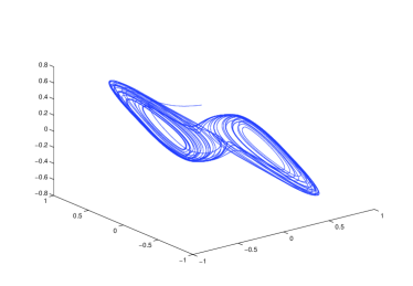
In this section, we give some numerical examples to illustrate the theoretical results. In these examples, we consider three-dimensional neural network as the uncoupled node dynamics [27]:

$$\frac{dx}{dt}=-Dx+Tg(x)$$ (17)

with $x=(x_{1},x_{2},x_{3})^{\top}\in\mathbb{R}^{3}$,

$\displaystyle T=\left[\begin{array}[]{ccc}1.2500&-3.200&-3.200\\ -3.200&1.100&-4.400\\ -3.200&4.400&1.000\end{array}\right]$

$D=I_{3}$ and $g(x)=(g(x_{1}),g(x_{2}),g(x_{3}))^{\top}$ where $g(s)=(|s+1|-|s-1|)/2$. This system has a double-scrolling chaotic attractor shown in Fig.1 with initial condition $x_{1}(0)=x_{2}(0)=x_{3}(0)=0.1000.$ In the following, we suppose system (17) is the uncoupled dynamical system of each agents and the inner coupling matrix $\Gamma=I_{n}$. We can find that any $\alpha>0.5$ can satisfy the decreasing condition with $G=I_{n}$. We use the following quantity to measure the variance for vertices and target trajectory:

$\displaystyle\varsigma(t)=\max_{i}\|x^{i}(t)-s(t)\|_{1}$

here for a vector $z=[z_{1},\cdots,z_{n}]^{\top}\in\mathbb{R}^{n}$, denote $\|z\|_{1}\hat{=}\max_{i}|z_{i}|$.

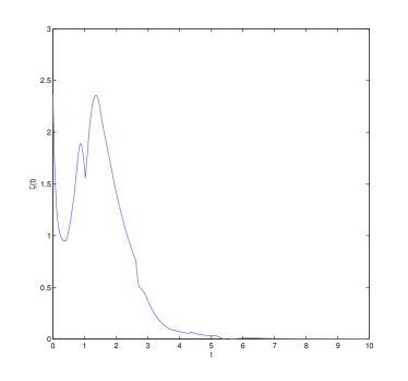
5.1 Slow switching among stable sub-systems

This simulation is for the pinning controlled network (4) under assumption in theorem 2 with $m=5$. The transition matrix $T$ of the Markov chain $\sigma_{t}$ is

$\displaystyle T=\left[\begin{array}[]{ccccc}0&0.65&0&0.35&0\\ 0&0&0.7&0&0.3\\ 0&0.1&0&0.9&0\\ 0.4&0.6&0&0&0\\ 0&0.3&0&0.7&0\end{array}\right].$

Pick the coupling matrices

$$L(1)=\left[\begin{array}[]{ccccc}-3&0&1&1&1\\ 0&-2&0&1&1\\ 1&1&-3&0&1\\ 0&0&0&-1&1\\ 1&1&0&0&-2\end{array}\right]$$
$$L(2)=\left[\begin{array}[]{ccccc}-2&0&0&1&1\\ 1&-2&0&0&1\\ 0&1&-2&0&1\\ 0&1&0&-2&1\\ 0&0&0&1&-1\end{array}\right]$$
$$L(3)=\left[\begin{array}[]{ccccc}-3&0&1&1&1\\ 1&-1&0&0&0\\ 1&0&-2&0&1\\ 0&0&0&-1&1\\ 1&1&1&1&-4\end{array}\right]$$
$$L(4)=\left[\begin{array}[]{ccccc}-2&1&0&0&1\\ 1&-2&0&0&1\\ 0&1&-3&1&1\\ 0&1&1&-2&0\\ 1&0&0&1&-2\end{array}\right]$$
$$L(5)=\left[\begin{array}[]{ccccc}-2&1&1&0&0\\ 0&-3&1&1&1\\ 1&1&-4&1&1\\ 0&1&1&-3&1\\ 0&1&1&1&-3\end{array}\right]$$

and the pinning control matrices

$$C(1)=diag\{1,1,0,0,1\}$$
$$C(2)=diag\{1,1,1,1,1\}$$
$$C(3)=diag\{0,0,0,1,1\}$$
$$C(4)=diag\{0,1,0,1,0\}$$
$$C(5)=diag\{1,1,1,0,0\}$$

Pick $P_{i}=I_{m},\alpha=1,\beta=0.5$, $k=10$ and $\epsilon=1$, then $\{\alpha I_{m}+kL(i)-k\epsilon C(i)\}^{s}$ are negative definite and $\{\alpha I_{m}+kL(i)-k\epsilon C(i)\}^{s}\leq-0.75I_{m}$. In case $\max_{i}{q_{i}}<0.75$, the condition in Theorem 1 is satisfied. Choose $q_{i}$ randomly in $(0,0.75)$. The initial value $x(0)$ and $s(0)$ are also chosen randomly. The ordinary different equations (4) are solved by the Runge-Kutta fourth-order formula with a step length of 0.01. Fig.2 indicates that the pinning control of (4) is stable.

Refer to caption
Figure 2: The dynamical behavior of $\varsigma(t)$.

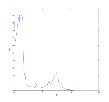
5.2 Locally pinning a system of mobile agents

In this simulation, we take the random waypoint mobility model [28] with $10$ agents. Suppose random waypoint area is square $\Lambda=\{(y_{1},y_{2})\in\mathbb{R}^{2}:0\leq y_{1}\leq 100,0\leq y_{2}\leq 100\}$, and the agents are randomly located in $\Lambda$, the control region $\Lambda_{c}=\{(y_{1},y_{2})\in\mathbb{R}^{2}:0\leq y_{1}\leq 50,0\leq y_{2}\leq 50\}$. The initial location of each agent is randomly chosen in $\Lambda$. If an agent achieves its target, it will stay in this location during a randomly chosen time interval $a$. If the distance between locations of two agents is less than 10, then these two agents are coupled. If the location of an agent is in $\Lambda_{c}$ at time $t$, then this agent is pinned at time $t$. Here, we pick $\alpha-\beta=0.5,P=I_{m}$. In this simulation, we can calculate the expected matrices $\bar{L}=[\bar{l}_{ij}]$ with $\bar{l}_{ij}=\frac{\pi 10^{2}}{100^{2}}\approx 0.0314$ for iβ‰ j𝑖𝑗i\neq j, $\bar{C}=0.25I_{m}$. Pick $\kappa\epsilon>0.5$ can guarantee $\alpha-0.25\kappa\epsilon\leq 0$. It can be calculated that $K_{1}=\beta,K_{2}\leq\alpha,K_{3}=\alpha-0.25\kappa\epsilon$. The Lipschitz constant of function $-Dx+Tg(x)$ is $Lf=4.68$. Pick $\kappa=0.5,\epsilon=12$, we can estimate that $K_{1}-K_{3}=1,K_{4}=2500,\rho=33$. If we take $\Delta=0.0004$, the condition (3) is guaranteed. Pick $r=750$. Hence, the minimum moving velocity $\underline{v}$ and maximum waiting time $\bar{t}_{w}$ should satisfy $\frac{d}{\bar{p}\underline{v}}+\frac{(1-\bar{p})\bar{t}_{w}}{\bar{p}}<r\Delta$ and $\frac{\tilde{d}}{\tilde{p}\underline{v}}+\frac{(1-\tilde{p})\bar{t}_{w}}{\tilde{p}}<r\Delta$, here the probabilities can be estimated: $\bar{p}>1-\frac{\pi r_{0}^{2}}{100^{2}}>0.99$ and $\tilde{p}=\frac{3}{4}$. Then, we obtain that $\underline{v}>500$ and $\bar{t}_{w}<0.33$. On the other hand, the maximum moving time is $\bar{t}_{m}=\frac{d}{\underline{v}}<0.29$ and we assume the waiting time larger than 0.29. The ordinary different equations (4) are solved by the Runge-Kutta fourth-order formula with a step length of 0.0001. Fig.3 indicates that the pinning control of (4) is stable.

Refer to caption
Figure 3: The dynamical behavior of $\varsigma(t)$.

6 Conclusion

In this paper, we investigate the pinning control problem of coupled dynamical systems with Markovian switching couplings and Markovian switching controller-set. We derive analytical conditions for the stability at the homogeneous trajectory of the uncoupled system. First, if each subsystem in the switching system with fixed pinning nodes can be stabilized and the Markovian switching is sufficiently slow, the system van be stabilized. Second, the switching system can be stabilized if the system with average coupling matrix and pinning gains can be stabilized and the Markovian switching is sufficiently fast. As an application, we also study the spatial pinning control problem of network with mobile agents. The effectiveness of the proposed theoretical results are demonstrated by two numerical examples.

References

  • [1] D. J. Watts, S. H. Strogatz, Collective Dynamics of Small World Networks, Nature, 393(1998):440-442.
  • [2] A. L. Barabasi, R. Albert, Emergence of Scaling in Random Networks, Science, 286(1999): 509-512.
  • [3] X. F. Wang, G. Chen, Pinning control of scale-free dynamical network, Physical A, 310(2002), 521-531.
  • [4] X. Li, X. F. Wang, G. Chen, Pinning a complex dynamical network to its equilibrium, IEEE Transactions on Circuits and Systems-I: regular paper, 51(10)(2004), 2074-2087.
  • [5] T. P. Chen, X. W. Liu, W. L. Lu, Pinning complex networks by a single controller. IEEE Transactions on Circuits and Systems-I: regular papers, 54(6)(2007):1317-1326.
  • [6] M. Porfiri, M. di Bernardo, Criteria for global pinning-controllability of complex network, Automatica, 44(2008), 3100-3106.
  • [7] W. W. Yu, G. Chen, J. H. LΓΌ, On pinning synchronization of complex dynamical networks, Automatica, 45(2009), 429-435.
  • [8] W. L. Lu, X. Li, Z. H. Rong, Global synchronization of complex networks with digraph topologies via a local pinning algorithm, Automatica 46(2010), 116-121.
  • [9] W. L. Lu, B. Liu, T. P. Chen, Cluster synchronization in networks of coupled nonidentical dynamical systems, Chaos, 20(2010), 013120 .
  • [10] W. Ren, Multi-vehicle consensus with a time-varying reference state, Systems Control Lett. 56 (2007) 474-483.
  • [11] Q. Song, J. D. Cao and W. W. Yu, Second-order leader-following consensus of nonlinear multi-agent systems via pinning control, Systems Control Lett. 59 (2010) 553-562.
  • [12] H. Y. Liu, G. M. Xie, L. Wang, Containment of linear multi-agent systems under general interaction topologies, Systems Control Letters, 61 (2012) 528-534.
  • [13] G. H. Wen, W. W. Yu, Y. Zhao, J. D. Cao, Pinning synchronization in fixed and switching directed networks of Lorenz-type nodes, IET Control Theory and Applications, 2013.
  • [14] L. Arnold, Stochastic differential equations: Theory and applications, John wiley sons, 1972.
  • [15] A. Friedman, Stochastic differential equations and their applications, vol. 2, Academic press, 1976.
  • [16] R. Z. Has’minskii, Stochastic stability of differential equations, Sijthoff and Noorrdhoff, 1981.
  • [17] V. B. Kolmanovskii, A. Myshkis, Applied theory of functional differential equations, Kluwer Academic Publishers, 1992.
  • [18] Y. Ji, H. J. Chizeck, Controllability, stabilizability and continuous-time Markovian jump linear quadratic control, IEEE Trans. Automat. Control 35(1990), 777-788.
  • [19] G. K. Basak, A. Bisi, M. K. Ghosh, Stability of a random diffusion with linear drift, J. Math. Anal. Appl. 202(1996), 604-622.
  • [20] X.R. Mao and C.G. Yuan, Stochastic differential equations with Markovian switching, Imperial College Press, 2006.
  • [21] C. G. Yuan, X. R. Mao, Robust stability and controllability of stochastic differential delay equations with Markovian switching, Automatica 40(2004), 343-354.
  • [22] X. F. Wang, X. Li, J. L$\ddot{u}$, Control and flocking of networked systems via pinning, IEEE Circuits and Systems, (2010), 83-91.
  • [23] H. Su, X.F. Wang, G. Chen, Flocking of multi-agents with a virtual leader, IEEE Transactions on Automatic Control, 54 (2009), 293-307.
  • [24] W. W. Yu, G. Chen, M. Cao, Distributed leader-follower flocking control for multi-agent dynamical systems with time-varying velocities, Systems Control Letters, 59 (2010) 543-552.
  • [25] M. Frasca, A. Buscarino, A. Rizzo, and L. Fortuna, Spatial Pinning Control, Physical Review Letters, 2012.
  • [26] G. L. Jones, On the Markov chain central limit theorem, Probability surveys, 1 (2004), 299-320.
  • [27] F. Zou, J.A. Nosse, Bifurcation, and chaos in cellular neural networks, IEEE Trans. CAS-1 40 (3) (1993) 166 C173.
  • [28] C. Bettstetter, H. Hartenstein, and X. Perez-Costa, Stochastic properties of the random waypoint mobility model, ACM/Kluwer Wireless Networks, to appear 2004.
  • [29] P. Bremaud, Markov Chains, Gibbs Fields, Monte Carlo Simulation, and Queues, 1999.
  • [30] P. Billingsley, Probability and Measure, Wiley, New York, 1986.
  • [31] N. wan de Wouw, and A. Pavlov, Tracking and synchronization for a class of PWA systems, Automatica, 44(11)(2008): 2909-2915.
  • [32] H. Kushner, Introduction to Stochastic Control, Holt, Rinehart and Winston, Inc., New York, NY, 1971.
  • [33] D. B. Johnson, D. A. Maltz. Dynamic source routing in ad hoc wireless networks. In Mobile computing, edited by T. Imielinski and H. Korth, chapter 5, pp. 153-181,Kluwer Academic Publishers, 1996.
  • [34] R. A. Horn and C. R. Johnson. Matrix analysis, Cambridge University Press, 1985.
  • [35] A. Berman, R. J. Plemmons, Nonnegative matrices in the mathematical sciences, SIAM, Philadelphia, PA, 1994.