Kondo effect in graphene with Rashba spin-orbit coupling

Abstract

We study the Kondo screening of a magnetic impurity adsorbed in graphene in the presence of Rashba spin-orbit interaction. The system is described by an effective single-channel Anderson impurity model, which we analyze using the numerical renormalization group. The nontrivial energy dependence of the host density of states gives rise to interesting behaviors under variation of the chemical potential or the spin-orbit coupling. Varying the Rashba coupling produces strong changes in the Kondo temperature characterizing the many-body screening of the impurity spin, and at half-filling allows approach to a quantum phase transition separating the strong-coupling Kondo phase from a free-moment phase. Tuning the chemical potential close to sharp features of the hybridization function results in striking features in the temperature dependences of thermodynamic quantities and in the frequency dependence of the impurity spectral function.

I Introduction

Two-dimensional “single-layer” materials have generated great attention over the past decade Novoselov et al. (2005); Castro Neto et al. (2009). Understanding the physics of these low-dimensional systems is highly desirable for the design of a new generation of electronic devices with on-demand characteristics. Single- or few-layer structures facilitate control by chemical and/or electrical means, as well as direct access to electronic features using local probes such as scanning tunneling microscopy Wiesendanger and Anselmetti (1992).

Coupling between orbital and spin degrees of freedom has noticeable effects on the properties of many single-layer materials. Spin-orbit interaction (SOI) can come into play either in its intrinsic form arising from the presence of constituent atoms with high atomic number, for instance in transition-metal dichalcogenides, or in extrinsic form due to the breaking of the electron spin degeneracy through spatial-inversion asymmetry arising from a substrate or an external electric field. The control and manipulation of SOI is also important for spintronics applications Yazyev (2010).

One fascinating direction relates to the physics of localized magnetic moments on single-layer structures and their collective screening through the Kondo effect Hewson (1993). This topic is of particular interest in the context of graphene, the prototypical single-layer material and perhaps the most basic condensed-matter system to feature low-energy Dirac fermions. Many analytical and a few experimental studies have recently reported controversial and sometimes conflicting results Fritz and Vojta (2013); Jobst et al. (2013) concerning the existence and nature of the Kondo effect. Among other suggestions has been the exciting possibility of accessing a regime of non-Fermi liquid multichannel Kondo physics Mattos et al. ; Sengupta and Baskaran (2008); Kharitonov and Kotliar (2013).

The goal of this paper is to advance understanding of the Kondo physics of a magnetic impurity adsorbed on graphene, properly taking into account Rashba SOI. Each of the important ingredients of this problem has been considered previously, but hitherto they have not all been treated within a single setting.

The effect of Rashba SOI on Kondo screening in conventional two-dimensional electron gases has been analyzed via a number of methods in the recent literature Malecki (2007); Žitko and Bonča (2011); Feng and Zhang (2011); Zarea et al. (2012); Isaev et al. (2012). It has been shown, in particular, that the Kondo temperature can be exponentially enhanced when the chemical potential is tuned to lie close to a van Hove singularity that arises in the density of states (DOS) due to SOI Wong et al. . This is an illustration of how nontrivial structure in the single-particle DOS can greatly impact the Kondo many-body effect.

In the absence of SOI, it is expected that magnetic-impurity physics in pristine graphene will reflect a linear vanishing of the DOS around the energy of the Dirac points, corresponding to the case $r=1$ of a pseudogap DOS in which $\rho(E)\propto|E-E_{F}|^{r}$ for energies $E$ close to the Fermi energy $E_{F}$. The pseudogap Kondo and Anderson models (first studied in the context of unconventional superconductivity, narrow-gap semiconductors, and flux phases) have interesting phase diagrams that depend on the strength of coupling between the impurity and the conduction band, as well as the presence or absence of particle-hole ($p$-$h$) symmetry Withoff and Fradkin (1990); Ingersent (1996); Bulla et al. (1997); Gonzalez-Buxton and Ingersent (1998).

Even though SOI is weak for graphene deposited on conventional substrates, it has been recently shown Marchenko et al. (2012) that Au intercalation at the interface between graphene and an Ni substrate can give rise to a spin-orbit splitting as large as $100$ meV. A large SOI has also been achieved in hydrogenated graphene at low concentrations, with Rashba coupling in the meV range Balakrishnan et al. (2013). The effect of Rashba SOI is to transform the linear band dispersion around each Dirac point into a four-band hyperbolic dispersion, generating discontinuities in the DOS at energies depending on the Rashba coupling parameter. SOI also converts to a nonzero DOS what in the absence of SOI would be a vanishing value at the charge-neutrality point, while still preserving a strong energy dependence.

Isolated magnetic moments can be generated in graphene either by decorating the sample with adatoms or molecules, or with vacancies produced by irradiation Ugeda et al. (2010). Most density functional (DFT) studies suggest that transition metals adatoms tend to prefer adsorption at hollow sites in the center of hexagons Mao et al. (2008); Sevinçli et al. (2008); Zanella et al. (2008); Johll et al. (2009); Krasheninnikov et al. (2009); Cao et al. (2010); Valencia et al. (2010); Sargolzaei and Gudarzi (2011); Ding et al. (2011); Zhang et al. (2013). However, it has been shown that the adsorption site is strongly influenced by the value of the local Coulomb interaction as reported by GGA+U calculations Wehling et al. (2011). Additionally, recent experimental works show that the adsorption site for Co and Ni atoms depends strongly on the substrate: Co always adsorbs onto SiC on top of a carbon atom, while for freestanding graphene one finds top and hollow sites for both Co and Ni Eelbo et al. (2013a); *EelboB2013. While adsorbed Ni always seems to be nonmagnetic, Co carries a magnetic moment that depends on the adsorption site.

In this paper we study an Anderson impurity model describing a configuration in which a spin-$\frac{1}{2}$ adatom with axial orbital symmetry is adsorbed on top of a graphene carbon atom, the most probable adsorption site for Co Eelbo et al. (2013a); *EelboB2013. The hybridization between the magnetic impurity and graphene bulk states inherits nontrivial energy dependence from the DOS. Using the numerical renormalization-group (NRG) technique, we calculate thermodynamic and spectral quantities that enable us to characterize the Kondo physics under variation of the chemical potential and the Rashba coupling. If the system is held at half-filling, increasing the Rashba parameter from zero gives rise to a quantum phase transition. When the system is doped such that the Fermi level lies close to a discontinuity in the impurity-band hybridization function, the proximity of a new screening channel produces a suppression in the Kondo peak near the Fermi energy, as can be seen in the impurity spectral function. The Kondo temperature, which exhibits a strong dependence on band filling, undergoes a sudden change as the chemical potential crosses a jump in the hybridization function. Additionally, the impurity is found to make a negative low-temperature contribution to thermodynamic quantities such as the magnetic susceptibility and the entropy. This rich behavior is in principle accessible in experiments.

The remainder of the paper is organized as follows. Section II describes the model and its transformation into a form that can be solved using the NRG method. Results are presented in Sec. III, followed by discussion and our conclusions in Sec. IV.

II Model and identification of relevant screening channel

Our analysis is based on an Anderson Hamiltonian for a system in which massless Dirac fermions of the host graphene experience Rashba SOI and are coupled to a nondegenerate impurity level exhibiting axial symmetry about a direction perpendicular to the plane of the graphene. We show in this section how the resulting multichannel model can be reduced to a single-channel Hamiltonian via a sequence of canonical transformations on the fermionic degrees of freedom. These transformations allow the energy-dependent impurity hybridization function to be identified.

II.1 Model Hamiltonian

We start with a real-space tight-binding Hamiltonian for graphene:

$$H_{g}=-t\sum_{\mathbf{R},j,s}a_{s}^{{\dagger}}(\mathbf{R})\>b_{s}^{\phantom{{\dagger}}}(\mathbf{R}+\boldsymbol{\delta}_{j})+\text{H.c.},$$ (1)

where $a_{s}(\mathbf{R})$ [$b_{s}(\mathbf{R})$] destroys an electron with spin $z$ projection $\pm\frac{1}{2}$ for $s=\pm 1$ (alternatively $s=\,\uparrow\!/\!\downarrow$) on the sublattice-$A$ [sublattice-$B$] carbon atom in the unit cell centered at $\mathbf{R}$. Also, $t\simeq 3$ eV is the nearest-neighbor hopping, and $\boldsymbol{\delta}_{j}$ ($j=1$, $2$, $3$) are nearest-neighbor translation vectors of length $a\simeq 1.42$ Å lying in the $x$-$y$ plane. After an expansion around the two nonequivalent Dirac points, located in two-dimensional reciprocal space at wave vectors $\mathbf{K}_{\pm}=(\pm 4\pi/(3\sqrt{3}a),\,0)$, we arrive at the low-energy effective Hamiltonian

$$H_{g}^{\text{eff}}=\sum_{\mathbf{q}}\psi^{\dagger}(\mathbf{q})\>h_{g}(\mathbf{q})\>\psi(\mathbf{q}),$$ (2)

with (setting $\hbar=1$)

$$h_{g}(\mathbf{q})=\tau_{0}\otimes s_{0}\otimes(v_{F}\,\mathbf{q}\cdot\boldsymbol{\sigma}-\mu\sigma_{0}),$$ (3)

where $\mathbf{q}=\mathbf{k}-\mathbf{K}_{\tau}$ is the wave vector measured from the center of valley $\tau=\pm$, $v_{F}=3at/2$ is the Fermi velocity, $\mu$ is the chemical potential, $\boldsymbol{\sigma}=(\sigma_{x},\sigma_{y})$ is a vector of Pauli matrices acting on a sublattice pseudospin degree of freedom $\sigma=\pm 1$, and $\tau_{0}$, $s_{0}$, and $\sigma_{0}$ are the two-dimensional identity matrices in the valley, spin, and pseudospin spaces, respectively. The Hamiltonian matrix (3), written in a valley-isotropic representation Beenakker (2008) that allows one to treat both valleys on the same footing, was obtained by arranging the eight-component spinor $\psi(\mathbf{q})$ as

$$\psi(\mathbf{q})=\bigl{(}\psi_{+,\uparrow}(\mathbf{q})^{T},\>\psi_{+,\downarrow}(\mathbf{q})^{T},\>\psi_{-,\uparrow}(\mathbf{q})^{T},\>\psi_{-,\downarrow}(\mathbf{q})^{T}\bigr{)}^{T},$$ (4)

with $\psi_{+,s}=(a_{+,s}\,,\,b_{+,s})^{T}$ and $\psi_{-,s}=(b_{-,s}\,,\,-a_{-,s})^{T}$ being indexed by $\sigma=1$ or $-1$. Here, $a_{\tau,s}(\mathbf{q})$ [$b_{\tau,s}(\mathbf{q})$] is the annihilation operator in sublattice $A$ [$B$], valley $\tau$, spin $z$ projection $s/2$, and relative wave vector $\mathbf{q}$.

The Rashba term, arising from asymmetry of the potential along the $z$ axis, is written in the tight-binding representation as Kane and Mele (2005)

$$H_{R}=i\frac{\lambda_{R}}{a}\sum_{\mathbf{R},j,s,s^{\prime}}a_{s}^{{\dagger}}(\mathbf{R})\,[\mathbf{s}_{ss^{\prime}}\times\boldsymbol{\delta}_{j}]_{z}\>b_{s^{\prime}}^{\phantom{{\dagger}}}(\mathbf{R}+\boldsymbol{\delta}_{j})+\text{H.c.},$$ (5)

where $s_{x}$ and $s_{y}$ are Pauli matrices in the spin space. A low-energy reciprocal-space representation can be deduced through expansion of Eq. (5) about each Dirac point, or it can be introduced by symmetry arguments Kane and Mele (2005). To zeroth order in $q_{x}a$ and $q_{y}a$,

$$H_{R}^{\text{eff}}=\sum_{\mathbf{q}}\psi^{{\dagger}}(\mathbf{q})\,h_{R}\,\psi(\mathbf{q}),$$ (6)

with

$$h_{R}=\lambda\,\tau_{0}(\boldsymbol{s}\times\boldsymbol{\sigma})\cdot\hat{\mathbf{z}}=\lambda\,\tau_{0}\left(s_{x}\sigma_{y}-s_{y}\sigma_{x}\right).$$ (7)

where the sign and magnitude of the Rashba parameter $\lambda=3\lambda_{R}/2$ can be tuned in experiments via an electric field applied parallel or antiparallel to the $z$ axis. For convenience, we take $\lambda\geq 0$.

We consider a magnetic impurity level that adsorbs to the sublattice-$A$ carbon atom in the unit cell at $\mathbf{R}=\mathbf{0}$. The nondegenerate level of the isolated impurity atom can be described by

$$H_{\text{imp}}=\epsilon_{d}\sum_{s}n_{ds}+Un_{d\uparrow}n_{d\downarrow},$$ (8)

where $\epsilon_{d}$ is the impurity level energy relative to the chemical potential, $U$ is the onsite Coulomb repulsion, and $n_{ds}=d_{s}^{{\dagger}}d_{s}^{\phantom{{\dagger}}}$ with $d_{s}$ destroying an electron of spin $s$ in the impurity level. Assuming that electron tunneling to/from the impurity level takes place only through the nearest carbon $p_{z}$ orbital, mixing between the impurity and the host is captured in a hybridization Hamiltonian term

$$H_{\text{mix}}=V\sum_{s}d_{s}^{{\dagger}}\>a_{s}^{\phantom{{\dagger}}}(\mathbf{0})+\text{H.c.},$$ (9)

which, after the Fourier transformation and expansion in reciprocal space about the Dirac points yields

$$H_{\text{mix}}=\frac{V}{\sqrt{N_{c}}}\sum_{\tau,s,\mathbf{q}}d_{s}^{{\dagger}}\>a_{\tau,s}^{\phantom{{\dagger}}}(\mathbf{q})+\text{H.c.},$$ (10)

where $N_{c}$ is the number of unit cells in the graphene layer.

Our goal is to understand the low-energy physics of the Hamiltonian $H=H_{g}^{\text{eff}}+H_{R}^{\text{eff}}+H_{\text{imp}}+H_{\text{mix}}$ defined in Eqs. (2)–(4), (6)–(8), and (10). In order to accomplish this, it is helpful to perform several simplifications described in the next subsection.

II.2 Transformation of the model

Taking advantage of the axial symmetry of the impurity about the $z$ axis perpendicular to the graphene plane, it is convenient to expand in an angular momentum basisMalecki (2007)

$$a_{\tau,s}(\mathbf{q})=\frac{1}{\sqrt{2\pi q}}\sum_{m=-\infty}^{\infty}e^{im\theta}\>a_{\tau,s}^{m}(q),$$ (11)

where $q=|\mathbf{q}|$, $\theta=\arctan(q_{y}/q_{x})$, $m$ is the azimuthal quantum number, and the prefactor of the summation ensures the anticommutation of the new operators. With a similar expression for the operator $b_{\tau,s}$, it is convenient to define new 8-component spinors

$$\psi_{j}(q)=\bigl{(}\psi_{+,\uparrow}^{j}(q)^{T},\>\psi_{+,\downarrow}^{j}(q)^{T},\>\psi_{-,\uparrow}^{j}(q)^{T},\>\psi_{-,\downarrow}^{j}(q)^{T}\bigr{)}^{T}$$ (12)

with $\psi_{+,s}^{j}=\bigl{(}a_{+,s}^{j-s-1/2},\,b_{+,s}^{j-s+1/2}\bigr{)}^{T}$ and $\psi_{-,s}^{j}=\bigl{(}b_{-,s}^{j-s-1/2},$ $-a_{-,s}^{j-s+1/2}\bigr{)}^{T}$. Since each operator entering $\psi_{j}$ satisfies $m+\frac{1}{2}(\tau\sigma+s)=j$, this spinor acts to decrease by $j$ the total angular momentum defined as $J_{z}=L_{z}+\frac{1}{2}(\tau_{z}\sigma_{z}+s_{z})$.

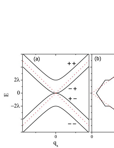
Figure 1: (Color online) (a) Graphene band structure near either Dirac point, plotted schematically as a function of $q_{x}$ for fixed $q_{y}=0$, where $\mathbf{q}=\mathbf{k}-\mathbf{K}_{\pm}$. Solid [dotted] lines represent the dispersion with [without] Rashba SOI. Each solid line is labeled with its $\alpha$, $\beta$ values. (b) The corresponding densities of states $\rho(E)$. For an impurity adsorbed directly on top of a carbon atom, the hybridization function $\Gamma(E)$ is simply proportional to $\rho(E)$.

With integration over $\theta$, the angular component of $\mathbf{q}$, the bulk Hamiltonian $H_{0}^{\text{eff}}\equiv H_{g}^{\text{eff}}+H_{R}^{\text{eff}}$ can be rewritten

$$H_{0}^{\text{eff}}=\sum_{j=-\infty}^{\infty}\int\!\!dq\;\psi_{j}^{{\dagger}}(q)\;[\tau_{0}s_{0}(v_{F}q\,\sigma_{x}-\mu\sigma_{0})+h_{R}]\;\psi_{j}^{\phantom{{\dagger}}}(q),$$ (13)

with $h_{R}$ still given by Eq. (7). This Hamiltonian can be put into the diagonal form

$$H_{0}^{\text{eff}}=\sum_{\alpha,\beta,\tau,j}\int\!dq\>\bigl{[}E_{\alpha,\beta}(q)-\mu\bigr{]}\,[f^{j}_{\alpha,\beta,\tau}(q)]^{{\dagger}}\,f^{j}_{\alpha,\beta,\tau}(q),$$ (14)

where $\alpha$ and $\beta$ run independently over $\pm$, and

$$E_{\alpha,\beta}(q)=\alpha\lambda+\beta\sqrt{(v_{F}q)^{2}+\lambda^{2}}.$$ (15)

The dispersions $E_{\alpha,\beta}(q)$ are shown schematically in Fig. 1(a), along with the corresponding dispersions for $\lambda=0$. Interestingly, the $\lambda\neq 0$ band structure is similar to that in Bernal-stacked bilayer graphene Castro et al. (2010) with $\lambda\rightarrow t_{\perp}/2$ (where $t_{\perp}$ is the interlayer hopping), although in the present case the presence of SOI also generates a nontrivial spin structure Rashba (2009). The DOS for each $(j,\tau)$ sector is

$$\rho(E)=\frac{\Omega_{0}}{\pi v_{F}^{2}}\bigl{[}|E|+\lambda+(|E|-\lambda)\>\Theta(|E|-2\lambda)\bigr{]},$$ (16)

where $\Theta(x)$ is the Heaviside step function. This DOS has a linear energy dependence with discontinuities at $E=\pm 2\lambda$, as shown schematically in Fig. 1(b).

We note that terms of higher order in $q_{x}a$ and $q_{y}a$ than those contained in Eqs. (2) and (6) modify Eqs. (15) and (16), both at energies $|E|\gtrsim t/10$ too high to play any essential part in the Kondo physics and below an energy scale proportional to $\lambda^{4}/t^{3}$ (see Ref. Zarea and Sandler, 2009). The effect of the low-energy departures from Eqs. (15) and (16) will be discussed in Sec. IV.

In the angular-momentum basis, the impurity-host hybridization Hamiltonian becomes

$$H_{\text{mix}}=V\sqrt{\frac{\Omega_{0}}{2\pi}}\sum_{s}d_{s}^{{\dagger}}\,\int\!dq\>\sqrt{q}\,a_{\tau,s}^{0}(q)+\text{H.c.},$$ (17)

where $\Omega_{0}$ is the graphene unit cell area. It is evident that this term involves only orbital angular momentum $m=0$, but that when expressed in terms of total angular momentum eigenstates, the impurity couples to $j=0$, $\pm 1$. Moreover, we need to express the operators $a_{\tau,s}^{0}$ in terms of the operators $f^{j}_{\alpha,\beta,\tau}$ that diagonalize $H_{0}^{\text{eff}}$.

It is straightforward to show that

$$\begin{split}a^{m}_{+,\uparrow}(q)&=-i\sum_{\alpha,\beta}\frac{\alpha}{N_{\alpha,\beta}(q)}f^{m+1}_{\alpha,\beta,+}(q),\\ b^{m}_{+,\uparrow}(q)&=-i\sum_{\alpha,\beta}\frac{\alpha E_{\alpha,\beta}(q)}{v_{F}q\,N_{\alpha,\beta}(q)}f^{m}_{\alpha,\beta,+}(q),\\ a^{m}_{+,\downarrow}(q)&=\sum_{\alpha,\beta}\frac{E_{\alpha,\beta}(q)}{v_{F}q\,N_{\alpha,\beta}(q)}f^{m}_{\alpha,\beta,+}(q),\\ b^{m}_{+,\downarrow}(q)&=\sum_{\alpha,\beta}\frac{1}{N_{\alpha,\beta}(q)}f^{m-1}_{\alpha,\beta,+}(q),\\ b^{m}_{-,\uparrow}(q)&=-i\sum_{\alpha,\beta}\frac{\alpha}{N_{\alpha,\beta}(q)}f^{m+1}_{\alpha,\beta,-}(q),\\ a^{m}_{-,\uparrow}(q)&=i\sum_{\alpha,\beta}\frac{\alpha E_{\alpha,\beta}(q)}{v_{F}q\,N_{\alpha,\beta}(q)}f^{m}_{\alpha,\beta,-}(q),\\ b^{m}_{-,\downarrow}(q)&=\sum_{\alpha,\beta}\frac{E_{\alpha,\beta}(q)}{v_{F}q\,N_{\alpha,\beta}(q)}f^{m}_{\alpha,\beta,-}(q),\\ a^{m}_{-,\downarrow}(q)&=-\sum_{\alpha,\beta}\frac{1}{N_{\alpha,\beta}(q)}f^{m-1}_{\alpha,\beta,-}(q),\end{split}$$ (18)

where

$$N_{\alpha,\beta}(q)=\sqrt{2}\left[1+\left(\frac{E_{\alpha,\beta}(q)}{v_{F}q}\right)^{2}\right]^{1/2}$$ (19)

ensures that the $f$ operators obey the canonical anticommutation relations

$$\bigl{\{}f^{j}_{\alpha,\beta,\tau}(q),f^{j^{\prime}}_{\alpha^{\prime},\beta^{\prime},\tau^{\prime}}(q^{\prime})^{{\dagger}}\bigr{\}}\\ =\delta_{\alpha,\alpha^{\prime}}\,\delta_{\beta,\beta^{\prime}}\,\delta_{\tau,\tau^{\prime}}\,\delta_{j,j^{\prime}}\,\delta(q-q^{\prime}).$$ (20)

Inserting Eqs. (18) into Eq. (17), we get

$$\begin{split}H_{\text{mix}}=&\;V\sqrt{\frac{\Omega_{0}}{2\pi}}\sum_{\alpha,\beta,\tau,s}\tau\,(-i\alpha)^{(1+s)/2}\>d_{s}^{{\dagger}}\int\!dq\>\frac{\sqrt{q}}{N_{\alpha,\beta}(q)}\\ &\;\times\left(\frac{E_{\alpha,\beta}(q)}{q}\right)^{(1-\tau s)/2}f^{(\tau+s)/2}_{\alpha,\beta,\tau}(q)+\text{H.c.}\end{split}$$ (21)

At this point, it is convenient to change from integration over wave vector $q$ to integration over energy $E$. We introduce a function $\Lambda_{\alpha,\beta}(E)=\Theta(\beta E-2\lambda\delta_{\alpha,\beta})$, which takes the value 1 for any value of $E$ for which there is a value of $q$ such that $E_{\alpha,\beta}(q)=E$, and which is zero otherwise. Then we can define new annihilation operators

$$f^{j}_{\alpha,\beta,\tau}(E) =|dq/dE|\>f^{j}_{\alpha,\beta,\tau}(q)$$

$$=\sqrt{\frac{\Lambda_{\alpha,\beta}(E)\,|E-\alpha\lambda|}{v_{F}\sqrt{E(E-2\alpha\lambda)}}}\>f^{j}_{\alpha,\beta,\tau}(q),$$ (22)

such that

$$\bigl{\{}f^{j}_{\alpha,\beta,\tau}(E),f^{j^{\prime}}_{\alpha^{\prime},\beta^{\prime},\tau^{\prime}}(E^{\prime})^{{\dagger}}\bigr{\}}\\ =\delta_{\alpha,\alpha^{\prime}}\,\delta_{\beta,\beta^{\prime}}\,\delta_{\tau,\tau^{\prime}}\,\delta_{j,j^{\prime}}\,\delta(E-E^{\prime}).$$ (23)

In the new basis,

$$H_{0}^{\text{eff}}=\sum_{\alpha,\beta,\tau,j}\int\!dE\>(E-\mu)\>f^{j}_{\alpha,\beta,\tau}(E)^{{\dagger}}f^{j}_{\alpha,\beta,\tau}(E),$$ (24)

and

$$H_{\text{mix}} =\frac{V}{2v_{F}}\sqrt{\frac{\Omega_{0}}{2\pi}}\!\sum_{\alpha,\beta,\tau,s}\!\!\tau\,(-i\alpha)^{(1+s)/2}\,d_{s}^{{\dagger}}\!\int\!\!dE\>\sqrt{\Lambda_{\alpha,\beta}(E)}$$

$$\times|E|^{(1-\tau s)/4}\,|E-2\alpha\lambda|^{(1+\tau s)/4}\,f^{(\tau+s)/2}_{\alpha,\beta,\tau}(E)+\text{H.c.}$$

$$=\frac{V}{2}\sum_{s}d_{s}^{{\dagger}}\int\!dE\>\sqrt{\rho(E)}\>g_{s}(E)+\text{H.c.},$$ (25)

where $\rho(E)$ is the density of states defined in Eq. (16) and

$$\begin{split}g_{s}(E)&=\sqrt{\frac{\Omega_{0}}{2\pi v_{F}^{2}\rho(E)}}\sum_{\alpha,\beta,\tau}\tau\,(-i\alpha)^{(1+s)/2}\,\sqrt{\Lambda_{\alpha,\beta}(E)}\\ &\times|E|^{(1-\tau s)/4}\,|E-2\alpha\lambda|^{(1+\tau s)/4}\,f^{(\tau+s)/2}_{\alpha,\beta,\tau}(E)\end{split}$$ (26)

satisfying

$$\bigl{\{}g_{s}^{\phantom{{\dagger}}}(E),g_{s^{\prime}}^{{\dagger}}(E^{\prime})\bigr{\}}=\delta_{s,s^{\prime}}\,\delta(E-E^{\prime})$$ (27)

is the annihilation operator for the single effective band or channel of host electrons that couples to the magnetic impurity. The Hamiltonian for the host can be rewritten

$$H_{0}^{\text{eff}}=\sum_{s}\int\!dE\>(E-\mu)\>g_{s}^{{\dagger}}(E)\,g_{s}^{\phantom{{\dagger}}}(E)+\ldots,$$ (28)

where “$\ldots$” describes degrees of freedom that do not couple to the impurity and which will henceforth be discarded.

Equations (8), (II.2), and (28) represent the reduction of the original four-channel Anderson model defined in Sec. II.1 to an effective one-channel Anderson impurity model having an impurity hybridization function

$$\Gamma(E)=\frac{\pi V^{2}}{4}\,\rho(E)$$ (29)

that is directly proportional to the DOS $\rho(E)$ shown in Fig. 1(b). It should be noted that even though spin is not a good quantum number in the presence of SOI, the DOS and thehybridization function entering the effective Anderson model are spin-independent.

The nontrivial energy dependence of the hybridization function, with linear regions separated by jumps, suggests that the Kondo physics will exhibit interesting modulations under variation of the chemical potential $\mu$ and/or the Rashba parameter $\lambda$. As noted in Sec. I, the DOS of graphene without SOI has the pseudogap form $\rho(E)\propto|E|^{r}$ with $r=1$. It is well established that for $\mu=0$ and $r\geq\frac{1}{2}$, and in the presence of $p$-$h$ symmetry, no Kondo screening is possible for any value $V$ of the hybridization Gonzalez-Buxton and Ingersent (1998); Fritz and Vojta (2013); instead, the system lies in a free-moment phase in which the ground state contains a free impurity spin entirely decoupled from the host. As soon as the Rashba SOI is turned on, however, the DOS at $E=0$ acquires a finite value $\Omega_{0}\lambda/\pi v_{F}^{2}$ [Eq. (16) and Fig. 1]. At fixed $\mu=0$, therefore, we expect the free-moment phase present for $\lambda=0$ to be replaced for $\lambda>0$ by a Kondo-screened phase with a Kondo temperature scale that varies exponentially with $-1/\lambda$. On the other hand, for fixed Rashba coupling, we expect a rapid change in the Kondo temperature as $\mu$ crosses the discontinuity in the hybridization function at $E=\pm 2\lambda$. As will be shown in the next section, these expectations are borne out by numerical calculations that also reveal other striking behaviors under variation of $\lambda$ and $\mu$.

III Numerical Results

We have performed numerical renormalization-group (NRG) calculations in order to rigorously test and quantify the qualitative expectations outlined at the end of Sec. II. The NRG is a nonperturbative method that allows the iterative diagonalization of the Hamiltonian for a quantum impurity model and yields reliable low-energy many-body states Wilson (1975); Bulla et al. (2008). These states can be used to calculate dynamical properties such as the impurity spectral function, as well as the impurity contribution to a thermodynamic property, defined to be $X_{\text{imp}}=X-X_{0}$ where $X$ is the value of the property in the full system consisting of the impurity coupled to the host, and $X_{0}$ is the corresponding value for the host alone.

We adopt units where $\hbar=k_{B}=g\mu_{B}=D=1$. All results shown are for the case of a $p$-$h$-symmetric impurity (i.e., $U=-2\epsilon_{d}$) with $U=0.02$, and for a hybridization-function prefactor $\Gamma_{0}\equiv\Omega_{0}DV^{2}/(4v_{F}^{2})=0.04$ or $0.08$. The data were calculated using an NRG discretization parameter $\Lambda=2.5$, retaining 2 000 many-body states after each iteration.

III.1 Kondo temperature

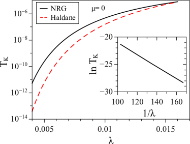
Figure 2: (Color online) Kondo temperature $T_{K}$ vs Rashba parameter $\lambda$ for chemical potential $\mu=0$ and hybridization prefactor $\Gamma_{0}=0.08$, comparing NRG calculations (solid line) with Haldane’s formula Eq. (30) (dashed line). The inset makes clear the exponential dependence of $T_{K}$ on $1/\lambda$, characteristic of a Kosterlitz-Thouless quantum phase transition.

We determine the Kondo temperature using the standard operational definition $T_{K}\chi_{\text{imp}}(T_{K})=0.0701$ based on the universal scaling of the impurity contribution to the static magnetic susceptibility of the Kondo model.Wilson (1975)

Figure 2 plots the Kondo temperature $T_{K}$ as a function of the Rashba parameter for the case $\mu=0$ where $\Gamma(E)$ takes its minimum value at $E=\mu$. The figure also shows the prediction

$$T_{K}=\sqrt{U\Gamma(\mu)/2}\>\exp\left[-\pi U/8\Gamma(\mu)\right]$$ (30)

obtained from Haldane’s formula Haldane (1978) for the Kondo temperature of an Anderson model with a flat hybridization function $\Gamma(E)=\Gamma(\mu)\,\Theta(D-|E|)$. The inset to Fig. 2 establishes the exponential dependence of $T_{K}$ on $1/\lambda$. The exponential vanishing $T_{K}$ as $\lambda\rightarrow 0$ is a signature of a quantum phase transition of Kosterlitz-Thouless type Hofstetter and Schoeller (2001); Vojta et al. (2002); Wong et al. (2012) at $\lambda=0$. That the NRG yields a larger $T_{K}$ than given by the Haldane formula, especially at low $\lambda$, is the result of the true hybridization function [Eq. (29)] satisfying $\Gamma(E)>\Gamma(\mu)$ for all $E\neq 0$.

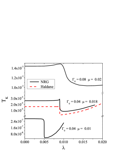
Figure 3: (Color online) Kondo temperature $T_{K}$ vs Rashba parameter $\lambda$ for three different combinations of the hybridization prefactor $\Gamma_{0}$ and the chemical potential $\mu$ that, for $\lambda=0$, take the system from its mixed valence regime [largest value of $\Gamma(\mu)$, top case] to deep in its Kondo regime [smallest $\Gamma(\mu)$, bottom case]. Solid lines plot NRG results, while the dashed line shows the prediction of Eq. (30) for the middle value of $\Gamma(\mu)$.

Figure 3 shows examples of the variation of $T_{K}$ with $\lambda$ away from the charge-neutrality point. Data are presented for three different combinations of $\Gamma_{0}$ and $\mu$. In each case, the Kondo temperature is almost constant as the Rashba parameter increases from zero until there is a rapid drop in $T_{K}$ centered close to $\lambda=|\mu|/2$. Further increase of $\lambda$ causes $T_{K}$ to rise and eventually surpass its value for $\lambda=0$. As shown for the case $\Gamma_{0}=0.04$, $\mu=0.018$, the main trends in the NRG results (solid lines) are captured quite well (dashed line) by Eq. (30) based on $\Gamma(\mu)=2\Gamma_{0}|\mu|/D$ for $\lambda<|\mu|/2$ and $\Gamma(\mu)=\Gamma_{0}(|\mu|+\lambda)/D$ for $\lambda>|\mu|/2$.

Figure 3 does show some deviations from the approximation in Eq. (30). First, just as in the case $\mu=0$ considered in Fig. 2, the formula systematically underestimates the Kondo temperature due to its neglect of regions of larger $\Gamma(E)$ far from the chemical potential. Second, the qualitative shape of the $T_{K}(\lambda)$ curve evolves with the degree of electronic correlation, which can be measured by the ratio $U/\pi\Gamma(\mu)=2.0$ (top case in Fig. 3), 4.4, and 8.0 (bottom case). In the most strongly correlated case, the NRG data show a downward rounding of $T_{K}(\lambda)$ for $\lambda$ just below $|\mu|/2$, whereas the other two cases exhibit a noticeable rise in $T_{K}$ as $\lambda$ approaches $|\mu|/2$ from below. These features, as well as a shift of the minimum in $T_{K}$ to a location $\lambda>|\mu|/2$, must arise from a subtle balance between increases and decreases in $\Gamma(E)$ over different decades of $|E-\mu|$. There is also a progressive smearing of sharp features in $T_{K}$ vs $\lambda$ as $U/\pi\Gamma(\mu)$ decreases, signaling a shift from pure-Kondo behavior (for which use of Haldane’s formula is justified) toward mixed valence (where the formula is inapplicable).

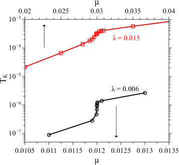
Figure 4: (Color online) Kondo temperature $T_{K}$ vs chemical potential $\mu$ near the jump in $\Gamma(\mu)$ at $\mu=2\lambda$, calculated for $\Gamma_{0}=0.04$ and two values of the Rashba parameter: $\lambda=0.006$ (circles, lower axis) and $\lambda=0.015$ (squares, upper axis). There is a rapid rise in $T_{K}$ as $\mu$ crosses the discontinuity in the hybridization function, with a sharper variation for the smaller $\lambda$.

Now we consider variation of the chemical potential at fixed Rashba parameter. There is a sharp jump $\Delta\Gamma(\mu)=\Gamma(0)\propto\lambda$ as $\mu$ rises through $2\lambda$. This jump manifests itself in a rapid increase in $T_{K}$ vs $\mu$, as shown in Fig. 4. For $\lambda=0.006$, the Kondo temperature rises by an order of magnitude as $\lambda$ increases by about 1%. For $\lambda=0.015$, the absolute values of $T_{K}$ and the size of the jump in $\Gamma(\mu)$ are larger than for $\lambda=0.006$, but the relative increase in $T_{K}$ on passing through $\mu=2\lambda$ is only half an order of magnitude. This can be understood from the fact that $\ln T_{K}\sim-1/\Gamma$, so $\partial\ln T_{K}/\partial\ln\Gamma\sim 1/\Gamma\sim 1/\lambda$, meaning that the change in $T_{K}$ due to the sharp variation of $\Gamma$ around $\mu=2\lambda$ is softened for increasing $\lambda$.

III.2 Thermodynamic and spectral quantities

We now turn to the variation with temperature $T$ of static impurity thermodynamic properties and to the frequency variation of $T=0$ dynamical quantities, considering situations where the chemical potential is close to a point where $\Gamma(\mu)$ jumps in value from $3\Gamma(0)$ to $4\Gamma(0)$. We focus on $\mu=2\lambda$, although the results would be identical for $\mu=-2\lambda$ due to the $p$-$h$ symmetry in the host and (for $U=-2\epsilon_{d}$) in the impurity.

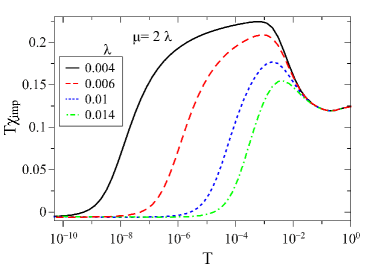
Figure 5: (Color online) Impurity contribution to the magnetic susceptibility at chemical potential $\mu=2\lambda$, calculated for $\Gamma_{0}=0.04$ and different values of the Rashba parameter $\lambda$. At low temperatures, $\chi_{\text{imp}}(T)$ changes sign, showing a residual negative susceptibility contribution as $T\rightarrow 0$.

Fig. 5 shows the magnetic susceptibility at $\mu=2\lambda$, plotted as $T\chi_{\text{imp}}$ vs $T$ for different values of the Rashba parameter ranging from $0.004$ to $0.014$. The curves exhibit features typical of Kondo screening, with $T\chi_{\text{imp}}$ increasing from near $1/8$ (the high-temperature susceptibility of the impurity level when decoupled from the host graphene) for $T\gg U,\,|\epsilon_{d}|$ toward its local-moment value $1/4$ in an intermediate temperature range before falling toward zero over four decades of temperature around $T_{K}$. However, it should be noted that $\lim_{T\to 0}T\chi_{\text{imp}}(T)$ is not zero, but rather negative. This distinctive property is associated with the sharp jump in $\Gamma(E)$, similar to behavior found in other systems where the hybridization function has a strong energy dependence Hofstetter and Kehrein (1999); Zhuravlev (2009); Zhuravlev and Irkhin (2011); Mastrogiuseppe et al. (2014). As $\chi_{\text{imp}}$ is the impurity contribution to the susceptibility, the negative values mean that the introduction of the magnetic adatom lowers the susceptibility compared to that of an impurity-free graphene layer.

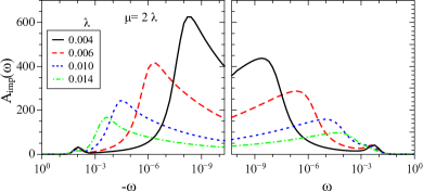
Figure 6: (Color online) Impurity spectral function $A_{\text{imp}}(\omega)$ vs frequency $\omega$ at $T=0$ for $\mu=2\lambda$, $\Gamma_{0}=0.04$, and different values of the Rashba parameter $\lambda$. The Kondo peak spanning $|\omega|\lesssim T_{K}$ is strongly asymmetric and features a sharp drop around the Fermi level due to the presence of the jump in $\Gamma(E)$ at $E=\mu$.

The impurity spectral function for $\mu=2\lambda$ plotted in Fig. 6 exhibits an asymmetric peak straddling the Fermi level ($\omega=0$), compatible with a Kondo resonance spanning the window $|\omega|\lesssim T_{K}$, but with a sharp dip superimposed that splits the peak into two parts. As we will see below, a similar feature appears even in the noninteracting case $U=0$, where it can be traced to the discontinuity in $\Gamma(E)$ at the chemical potential. As $\lambda$ increases, the combined “peak-dip” feature becomes wider, tracking the increase in $T_{K}$.

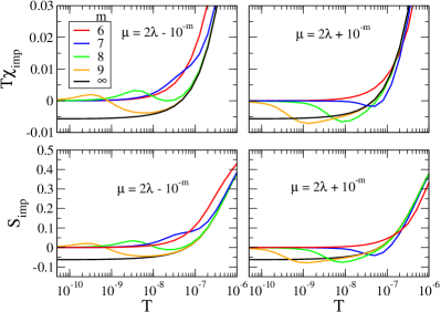
Figure 7: (Color online) Low-temperature variation of temperature times the impurity magnetic susceptibility $T\chi_{\text{imp}}$ (upper panels) and impurity entropy $S_{\text{imp}}$ (lower panels) for $\Gamma_{0}=0.04$, $\lambda=0.006$, and different values of the chemical potential $\mu=2\lambda\pm 10^{-m}$ close to a jump in $\Gamma(\mu)$.

Figures 7 and 8 show properties at fixed $\lambda=0.006$ for a set of chemical potentials $\mu=2\lambda\pm 10^{-m}$ with different integer values of $m$. When the chemical potential is sufficiently far from the discontinuity ($m\lesssim 6$), both $T\chi_{\text{imp}}$ and $S_{\text{imp}}$ show temperature dependences characteristic of Kondo screening and approach zero monotonically over the temperature range shown. As $\mu$ gets closer to the jump in $\Gamma(\mu)$, the low-temperature behavior changes in a way that depends on the sign of $\mu-2\lambda$. For $\mu<2\lambda$, $T\chi_{\text{imp}}$ and $S_{\text{imp}}$ both cross to negative values and then back to positive values before approaching zero from above as $T\rightarrow 0$. For $\mu>2\lambda$, by contrast, $T\chi_{\text{imp}}$ and $S_{\text{imp}}$ each change sign once and approach zero from below. The properties deviate from their counterparts for $\mu=2\lambda$ (i.e., $m\to\infty$) below a characteristic temperature scale $T^{*}\simeq|\mu-2\lambda|$. The range of $\mu$ in which unconventional behavior is found is essentially the one in which $T^{*}\lesssim T_{K}$.

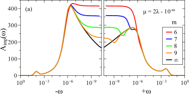
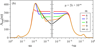
Figure 8: (Color online) Impurity spectral function $A_{\text{imp}}(\omega)$ vs frequency $\omega$ at $T=0$, calculated for $\Gamma_{0}=0.04$, $\lambda=0.006$, and different values of the chemical potential $\mu=2\lambda\pm 10^{-m}$ close to a jump in $\Gamma(\mu)$. For $T^{*}\simeq|\mu-2\lambda|\lesssim T_{K}$, the Kondo peak shows a dip near the location $\omega=2\lambda-\mu$ of the discontinuity.

The impurity spectral function for $\lambda=0.006$ and $\mu=2\lambda\pm 10^{-m}$ is shown in Fig. 8. For values of $\mu$ far enough from the discontinuity (as in the case $m=6$), there is a conventional, if slightly asymmetric, Kondo peak at the Fermi level. Once $\mu$ approaches the jump close enough that $T\chi_{\text{imp}}$ and $S_{\text{imp}}$ undergo sign changes (i.e., $T^{*}\simeq|\mu-2\lambda|\lesssim T_{K}$), the shape of $A_{\text{imp}}(\omega)$ is modified around the Fermi level. The peak loses spectral weight, particularly on the side satisfying $\omega\,(2\lambda-\mu)>0$. The value of $A_{\text{imp}}(0)$ drops, while $A_{\text{imp}}(T_{K})$ and $A_{\text{imp}}(-T_{K})$ change more slowly, resulting in splitting of the Kondo peak into two asymmetric parts around a minimum at $\omega\simeq(2\lambda-\mu)\simeq T^{*}\,\text{sgn}(2\lambda-\mu)$.

In order to gain insight into the nature of the unusual behavior reported above for $\mu$ near a discontinuity in the hybridization function, it is useful to consider the case $U=0$, for which the impurity spectral function may be expressed as Hewson (1993)

$$A_{\text{imp}}(\omega)=\frac{1}{\pi}\frac{\Gamma(\omega)}{[\omega-\epsilon_{d}-\Sigma^{\prime}_{d}(\omega)]^{2}+\Gamma(\omega)^{2}},$$ (31)

with $\Gamma(\omega)$ given by Eq. (29) and

$$\begin{split}\Sigma^{\prime}_{d}(\omega)&=\frac{1}{\pi}P\int\!d\omega^{\prime}\frac{\Gamma(\omega^{\prime})}{\omega-\omega^{\prime}}\\ &=\frac{V^{2}\Omega_{0}}{4\pi v_{F}^{2}}\Biggl{\{}(\omega+\mu)\biggl{[}2\log\bigg{|}\frac{(\omega+\mu)^{2}-4\lambda^{2}}{(\omega+\mu)^{2}-1}\bigg{|}\\ &-\log{\bigg{|}1-\frac{4\lambda^{2}}{(\omega+\mu)^{2}}\bigg{|}}\bigg{]}-\log{\bigg{|}\frac{\omega+\mu-2\lambda}{\omega+\mu+2\lambda}\bigg{|}}\Biggr{\}}.\end{split}$$ (32)

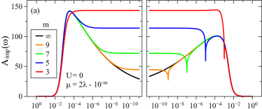
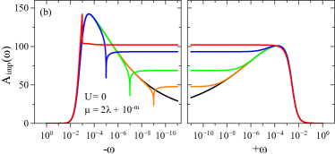
Figure 9: (Color online) Impurity spectral function $A_{\text{imp}}$ vs frequency $\omega$ at $T=0$ for the noninteracting case $U=0$ with $\epsilon_{d}=0.007$, $\Gamma_{0}=0.04$, $\lambda=0.015$, and different values of the chemical potential $\mu=2\lambda\pm 10^{-m}$ close to a jump in $\Gamma(\mu)$. A sharp, asymmetric dip structure is centered near the location $\omega=2\lambda-\mu$ of the discontinuity in the hybridization function.

Figure 9 shows the noninteracting spectral function $A_{\text{imp}}(\omega)$ for $\lambda=0.015$ and $\mu=2\lambda\pm 10^{-m}$. The impurity level energy is set to $\epsilon_{d}=0.007$ in order to have a resonance in the spectral function located near the Fermi level, playing the role analogous to a Kondo peak in the interacting case. Comparing this figure with the interacting one in Fig. 8, one observes many qualitative similarities. However, the dip in $A_{\text{imp}}(\omega)$ near the position $\omega=2\lambda-\mu$ of the hybridization function discontinuity appears much sharper for $U=0$ than in the interacting case, due to rescaling introduced by the interactions and NRG discretization effects.

One feature that is quantitatively similar between Figs. 8 and 9 is the asymmetry in the value of $A_{\text{imp}}(0)$ under reversal in the sign of $\mu-2\lambda$. For $\mu$ fairly far from the discontinuity in $\Gamma(\mu)$ (e.g., $m=6$ in the figures), the value of $A_{\text{imp}}(0)$ is one-third higher for $\mu<2\lambda$ than for $\mu>2\lambda$. Both for $U=0$ and for $U>0$, this can be understood in terms of approach to the flat-band limit in which the Friedel sum rule gives $A_{\text{imp}}(0)=1/[\pi\Gamma(\mu)]$. For smaller values of $|\mu-2\lambda|$, the nontrivial variation of $\Gamma(E)$ near $E=\mu$ modifies the form of the Friedel sum rule Dias da Silva et al. (2006) and leads to $A_{\text{imp}}(0)<1/[\pi\Gamma(\mu)]$.

We conclude from this comparison with the case $U=0$ that the principal features of the impurity spectral functions shown in Fig. 8 stem from the jump in the hybridization function. The dip or antiresonance in $A_{\text{imp}}$ at the location of the hybridization step is reminiscent of behavior found previously in systems with a gapped DOS Chen and Jayaprakash (1998); Galpin and Logan (2008, 2008); Moca and Roman (2010); Mkhitaryan and Mishchenko (2013); Mastrogiuseppe et al. (2014), where resonances of single-particle character can appear inside the gap due to the jump onset in the hybridization function at the the gap edge.

IV Discussion

We have presented a study of the Kondo screening of a nondegenerate magnetic impurity adatom on graphene in the presence of Rashba spin-orbit interaction. The impurity has been assumed to sit on top of a carbon atom, shown by recent experiments to be the most likely position for Co impurities. This configuration can be described by an Anderson impurity model in which a localized level mixes with a single effective band via an energy-dependent hybridization function $\Gamma(E)$ that is directly proportional to the graphene density of states and contains a pair of jumps whose magnitude is proportional to the Rashba strength $\lambda$, located at energies $E=\pm 2\lambda$.

We have analyzed different regimes that can be accessed by tuning the chemical potential $\mu$ and the Rashba strength $\lambda$. At $\mu=\lambda=0$ (only), $\Gamma(\mu)=0$ and hence for $\Gamma_{0}<\Gamma_{0,c}$ the system lies in a free-moment phase where the ground state contains a decoupled impurity spin. $\Gamma_{0,c}=\infty$ for the case $U=-2\epsilon_{d}$ considered in our calculations, but away from strict $p$-$h$ symmetry ($U\neq-2\epsilon_{d}$, not shown) the critical hybridization prefactor $\Gamma_{0,c}$ would be finite (Ref. Gonzalez-Buxton and Ingersent, 1998). For $\Gamma_{0}>\Gamma_{0,c}$ or for any nonzero value of $\mu$ and/or $\lambda$, the system instead lies in a strong-coupling (Kondo) phase in which the impurity degree of freedom is quenched at temperatures much below $T_{K}$. This Kondo scale is exponential in $-1/\Gamma(\mu)$, indicating that the singular point $\mu=\lambda=0$ is the location of a Kosterlitz-Thouless type of quantum phase transition.

When the chemical potential lies close to one of the jumps in $\Gamma(E)$, the impurity contributions to the static magnetic susceptibility and the entropy show unusual behavior with decreasing temperature, including a sign change (or even two) before Kondo screening ultimately sets in. Similar features have been predicted before in other situations where the hybridization function exhibits rapid or discontinuous energy dependence Hofstetter and Kehrein (1999); Dias da Silva et al. (2006); Zhuravlev (2009); Zhuravlev and Irkhin (2011); Mastrogiuseppe et al. (2014). In the same range of $\mu$, the impurity spectral function shows anomalies connected to those seen in the thermodynamic quantities. The Kondo peak is asymmetric about $\omega=0$ and for $|\mu-2\lambda|\lesssim T_{K}$ has a sharp dip-like structure, which can be traced back to a similar feature found in the noninteracting limit of the model.

Our results have been derived based on an effective description $H_{0}^{\text{eff}}=H_{g}^{\text{eff}}+H_{R}^{\text{eff}}$ [Eqs. (2) and (6)] of the host graphene, obtained via a low-order expansion of $H_{0}=H_{g}+H_{R}$ [Eqs. (1) and (5)] in powers of $q_{x}a$ and $q_{y}a$, where $\mathbf{q}=\mathbf{k}-\mathbf{K}_{\tau}$ is the deviation in reciprocal space from one or other of the two Dirac points $\tau=\pm$ found for $\lambda=0$. The effective description yields the hyperbolic band dispersions given in Eq. (15) and the density of states in Eq. (16) having a minimum value $\rho(0)=\Omega_{0}\lambda/\pi v_{F}^{2}>0$. However, it has been shown Zarea and Sandler (2009) that a complete analysis of $H_{0}=H_{g}+H_{R}$ yields a band structure that for $\lambda_{R}>0$ has six Dirac points, three in each valley $\tau=\pm$ at reciprocal space locations satisfying $|\mathbf{q}|a\simeq 2(\lambda_{R}/t)^{2}$. As a result, $\rho(E)$ deviates from the form given in Eq. (16) for $|E|<E_{1}\propto\lambda_{R}^{4}/t^{3}$, dropping linearly to zero at $E=0$ rather than approaching a nonzero limit.

As a consequence of the behavior $\rho(E)\propto|E|$ for $|E|\lesssim E_{1}$, when the system is tuned to half filling ($\mu=0$), the pseudogap condition $\Gamma(\mu)=0$ holds for all values of $\lambda=3\lambda_{R}/2$ (not just for $\lambda=0$ as found using $H_{0}^{\text{eff}}$). This means that for a $p$-$h$-symmetric impurity ($U=-2\epsilon_{d}$), the system always has a free-moment ground state, while in other cases the free-moment ground state holds for sufficiently weak impurity-host hybridization. It is important to note, though, that Kondo physics of an Anderson impurity in a host described by $H_{0}$ will differ from that reported in Sec. III for a system described by $H_{0}^{\text{eff}}$ only on temperature scales $T\lesssim E_{1}$. The impurity moment will in many cases appear to be quenched for $E_{1}\lesssim T\lesssim T_{K}$, where $T_{K}$ is the effective Kondo scale deduced using the low-order description $H_{0}^{\text{eff}}$, and only for $T\ll E_{1}$ will the many-body screening unwind to reveal an asymptotically free local impurity moment. For all physically plausible values of $\lambda_{R}$ (smaller than $10$ meV, say), $E_{1}$ will be orders of magnitude below the base temperature $T_{\text{min}}$ of any experiment, and there will be no detectable difference between results for $H_{0}$ and those for $H_{0}^{\text{eff}}$.

The physics we have described should be accessible through scanning tunneling microscopy on a graphene sample decorated with a few magnetic adatoms. To approach the quantum phase transition between the Kondo and free-moment phases, one could vary $\lambda$ at half filling by manipulating the substrate and/or the hydrogenation level, or by applying an electric field while keeping the graphene charge-neutral. Even though the free-moment phase is confined to $\mu=\lambda=0$ (at least within the effective description of the host provided by $H_{0}^{\text{eff}}$), in a real experiment the system would appear to display free-moment behavior once $\lambda$ becomes small enough that $T_{K}<T_{\text{min}}$. Another interesting regime of the system should be accessible via gate tuning of the chemical potential close to a jump in the host density of states. In systems with strong Rashba coupling (such as graphene on a Ni substrate with Au intercalation Marchenko et al. (2012) or hydrogenated samples Balakrishnan et al. (2013)), scanning tunneling spectroscopy should allow one to observe the characteristic dip structure in the spectral function. Although intercalation or decoration could induce disorder and modify the DOS, it has been observed that Au intercalation tends to decouple graphene from the Ni substrate, leading to a quasi-pristine graphene structure Marchenko et al. (2012).

In systems with more moderate Rashba coupling, it may be possible to observe a rapid change in $T_{K}$ as the chemical potential is varied by a few percent around $2\lambda$.

In conclusion, we find that Kondo screening in graphene is robust against the presence of Rashba spin-orbit interaction, even though this coupling breaks the spin symmetry of the Hamiltonian. Electrons with different projections 0, $\pm 1$ of the total angular momentum about an axis perpendicular to the graphene layer recombine to form a single effective band of screening fermions. The density of states of this band has a strong energy dependence that leads to nontrivial phenomena. Our results suggest experimental signatures that may also characterize the Kondo physics in the new generation of layered two-dimensional compounds where spin-orbit interactions plays an even stronger role.

References

- Novoselov et al. (2005) K. S. Novoselov, D. Jiang, F. Schedin, T. J. Booth, V. V. Khotkevich, S. V. Morozov, and A. K. Geim, Proc. Natl. Acad. Sci. U. S. A. 102, 10451 (2005).
- Castro Neto et al. (2009) A. H. Castro Neto, F. Guinea, N. M. R. Peres, K. S. Novoselov, and A. K. Geim, Rev. Mod. Phys. 81, 109 (2009).
- Wiesendanger and Anselmetti (1992) R. Wiesendanger and D. Anselmetti, STM on Layered Materials (Springer, Heidelberg, 1992) Chap. 6, pp. 131-179.
- Yazyev (2010) O. V. Yazyev, Rep. Prog. Phys. 73, 056501 (2010).
- Hewson (1993) A. Hewson, The Kondo Problem to Heavy Fermions (Cambridge University Press, New York, N.Y., 1993).
- Fritz and Vojta (2013) L. Fritz and M. Vojta, Rep. Prog. Phys. 76, 032501 (2013).
- Jobst et al. (2013) J. Jobst, F. Kisslinger, and H. B. Weber, Phys. Rev. B 88, 155412 (2013).
- (8) L. S. Mattos, C. R. Moon, M. W. Sprinkle, C. Berger, K. Sengupta, A. V. Balatsky, W. A. de Heer, and H. C. Manoharan, (unpublished).
- Sengupta and Baskaran (2008) K. Sengupta and G. Baskaran, Phys. Rev. B 77, 045417 (2008).
- Kharitonov and Kotliar (2013) M. Kharitonov and G. Kotliar, Phys. Rev. B 88, 201103(R) (2013).
- Malecki (2007) J. Malecki, J. Stat. Phys. 129, 741 (2007).
- Žitko and Bonča (2011) R. Žitko and J. Bonča, Phys. Rev. B 84, 193411 (2011).
- Feng and Zhang (2011) X.-Y. Feng and F.-C. Zhang, J. Phys.: Condens. Matter 23, 105602 (2011).
- Zarea et al. (2012) M. Zarea, S. E. Ulloa, and N. Sandler, Phys. Rev. Lett. 108, 046601 (2012).
- Isaev et al. (2012) L. Isaev, D. Agterberg, and I. Vekhter, Phys. Rev. B 85, 081107(R) (2012).
- (16) A. Wong et al., (in preparation).
- Withoff and Fradkin (1990) D. Withoff and E. Fradkin, Phys. Rev. Lett. 64, 1835 (1990).
- Ingersent (1996) K. Ingersent, Phys. Rev. B 54, 11936 (1996).
- Bulla et al. (1997) R. Bulla, T. Pruschke, and A. C. Hewson, J. Phys.: Condens. Matter 9, 10463 (1997).
- Gonzalez-Buxton and Ingersent (1998) C. Gonzalez-Buxton and K. Ingersent, Phys. Rev. B 57, 14254 (1998).
- Marchenko et al. (2012) D. Marchenko, A. Varykhalov, M. Scholz, G. Bihlmayer, E. Rashba, A. Rybkin, A. Shikin, and O. Rader, Nat. Commun. 3, 1232 (2012).
- Balakrishnan et al. (2013) J. Balakrishnan, G. Kok Wai Koon, M. Jaiswal, A. H. Castro Neto, and B. Ozyilmaz, Nat. Phys. 9, 284 (2013).
- Ugeda et al. (2010) M. M. Ugeda, I. Brihuega, F. Guinea, and J. M. Gómez-Rodríguez, Phys. Rev. Lett. 104, 096804 (2010).
- Mao et al. (2008) Y. Mao, J. Yuan, and J. Zhong, J. Phys.: Condens. Matter 20, 115209 (2008).
- Sevinçli et al. (2008) H. Sevinçli, M. Topsakal, E. Durgun, and S. Ciraci, Phys. Rev. B 77, 195434 (2008).
- Zanella et al. (2008) I. Zanella, S. B. Fagan, R. Mota, and A. Fazzio, J. Phys. Chem. C 112, 9163 (2008).
- Johll et al. (2009) H. Johll, H. C. Kang, and E. S. Tok, Phys. Rev. B 79, 245416 (2009).
- Krasheninnikov et al. (2009) A. Krasheninnikov, P. Lehtinen, A. Foster, P. Pyykko, and R. Nieminen, Phys. Rev. Lett. 102, 126807 (2009).
- Cao et al. (2010) C. Cao, M. Wu, J. Jiang, and H.-P. Cheng, Phys. Rev. B 81, 205424 (2010).
- Valencia et al. (2010) H. Valencia, A. Gil, and G. Frapper, J. Phys. Chem. C 114, 14141 (2010).
- Sargolzaei and Gudarzi (2011) M. Sargolzaei and F. Gudarzi, J. Appl. Phys. 110, 064303 (2011).
- Ding et al. (2011) J. Ding, Z. Qiao, W. Feng, Y. Yao, and Q. Niu, Phys. Rev. B 84, 195444 (2011).
- Zhang et al. (2013) T. Zhang, L. Zhu, S. Yuan, and J. Wang, ChemPhysChem 14, 3483 (2013).
- Wehling et al. (2011) T. O. Wehling, A. I. Lichtenstein, and M. I. Katsnelson, Phys. Rev. B 84, 235110 (2011).
- Eelbo et al. (2013a) T. Eelbo, M. Waśniowska, P. Thakur, M. Gyamfi, B. Sachs, T. O. Wehling, S. Forti, U. Starke, C. Tieg, A. I. Lichtenstein, and R. Wiesendanger, Phys. Rev. Lett. 110, 136804 (2013a).
- Eelbo et al. (2013b) T. Eelbo, M. Waśniowska, M. Gyamfi, S. Forti, U. Starke, and R. Wiesendanger, Phys. Rev. B 87, 205443 (2013b).
- Beenakker (2008) C. Beenakker, Rev. Mod. Phys. 80, 1337 (2008).
- Kane and Mele (2005) C. L. Kane and E. J. Mele, Phys. Rev. Lett. 95, 226801 (2005).
- Castro et al. (2010) E. V. Castro, K. S. Novoselov, S. V. Morozov, N. M. R. Peres, J. M. B. L. dos Santos, J. Nilsson, F. Guinea, A. K. Geim, and A. H. C. Neto, J. Phys.: Condens. Matter 22, 175503 (2010).
- Rashba (2009) E. I. Rashba, Phys. Rev. B 79, 161409 (2009).
- Zarea and Sandler (2009) M. Zarea and N. Sandler, Phys. Rev. B 79, 165442 (2009).
- Note (1) Similar reductions of multi-channel Anderson models to effective one-channel models have been performed previously in connection with Kondo physics in topological insulatorsŽitko and Bonča (2011) and in a two-dimensional electron gas with Rashba coupling [R. Zitko, Phys. Rev. B 81, 241414 (2010)].
- Wilson (1975) K. G. Wilson, Rev. Mod. Phys. 47, 773 (1975).
- Bulla et al. (2008) R. Bulla, T. A. Costi, and T. Pruschke, Rev. Mod. Phys. 80, 395 (2008).
- Note (2) More recent NRG advancesAnders and Schiller (2005); Weichselbaum and von Delft (2007) allow superior calculation of spectral properties and thermodynamics in magnetic fields. However, for the present work the standard method is satisfactory.
- Haldane (1978) F. D. M. Haldane, Phys. Rev. Lett. 40, 416 (1978).
- Hofstetter and Schoeller (2001) W. Hofstetter and H. Schoeller, Phys. Rev. Lett. 88, 016803 (2001).
- Vojta et al. (2002) M. Vojta, R. Bulla, and W. Hofstetter, Phys. Rev. B 65, 140405 (2002).
- Wong et al. (2012) A. Wong, W. B. Lane, L. G. G. V. Dias da Silva, K. Ingersent, N. Sandler, and S. E. Ulloa, Phys. Rev. B 85, 115316 (2012).
- Hofstetter and Kehrein (1999) W. Hofstetter and S. Kehrein, Phys. Rev. B 59, R12732 (1999).
- Zhuravlev (2009) A. K. Zhuravlev, Phys. Met. Metallogr. 108, 107 (2009).
- Zhuravlev and Irkhin (2011) A. K. Zhuravlev and V. Y. Irkhin, Phys. Rev. B 84, 245111 (2011).
- Mastrogiuseppe et al. (2014) D. Mastrogiuseppe, A. Wong, K. Ingersent, S. E. Ulloa, and N. Sandler, Phys. Rev. B 89, 081101(R) (2014).
- Dias da Silva et al. (2006) L. G. G. V. Dias da Silva, N. P. Sandler, K. Ingersent, and S. E. Ulloa, Phys. Rev. Lett. 97, 096603 (2006).
- Chen and Jayaprakash (1998) K. Chen and C. Jayaprakash, Phys. Rev. B 57, 5225 (1998).
- Galpin and Logan (2008) M. R. Galpin and D. E. Logan, Phys. Rev. B 77, 195108 (2008).
- Moca and Roman (2010) C. P. Moca and A. Roman, Phys. Rev. B 81, 235106 (2010).
- Mkhitaryan and Mishchenko (2013) V. V. Mkhitaryan and E. G. Mishchenko, Phys. Rev. Lett. 110, 086805 (2013).
- Anders and Schiller (2005) F. B. Anders and A. Schiller, Phys. Rev. Lett. 95, 196801 (2005).
- Weichselbaum and von Delft (2007) A. Weichselbaum and J. von Delft, Phys. Rev. Lett. 99, 076402 (2007).