Non-equilibrium Statistical Approach to Friction Models

Abstract

A geometric approach to the friction phenomena is presented. It is based on the holographic view which has recently been popular in the theoretical physics community. We see the system in one-dimension-higher space. The heat-producing phenomena are most widely treated by using the non-equilibrium statistical physics. We take 2 models of the earthquake. The dissipative systems are here formulated from the geometric standpoint. The statistical fluctuation is taken into account by using the (generalized) Feynman’s path-integral.

1 INTRODUCTION

The system we consider consists of the huge number of particles (blocks) and the size of the constituent particles is the mesoscopic-scale. It is lager than 50 nm =$5\times 10^{-8}$m and is far bigger than the atomic scale ($\sim 10^{-10}$m). It is smaller than or nearly equal to the optical microscope scale ($\sim 10^{-6}$m) in the branches such as the soft-matter physics, the nano-science physics and the biophysics. The larger end of the mesoscopic (length) scale depends on each phenomenon. For the earthquake it is about $10^{-4}$m.

The physical quantities, such as velocity, energy and entropy, are the statistically-averaged ones. It is not obtained by the deterministic way like the classical (Newton) mechanics. Renormalization phenomenon occurs not from the quantum effect but from the statistical fluctuation due to the uncertainty caused by the following facts. Firstly each particle obeys the Newton’s law with different initial conditions. The total number of particles, N, is so large that we do not or can not observe the initial data. Usually we do not have interest in the trajectory of every particle and do not observe it. We have interest only in the macroscopic quantities: total energy and total entropy are the most important ones. Secondly, in the real system, the size and shape differ particle by particle. We regard the randomness as a part of fluctuation. Finally the models, presented in the following, contains discrete parameters ($t_{n}$ in Sec.2 and $y_{n}$ in Sec.3). As far as the discreteness is kept (in the case that we no not take the continuous limit), the quantities determined by the minimal principle include the inevitable ambiguity which is regarded as a part of fluctuation.

After the development of the string and D-brane theories[1, 2], one general relation, between the 4-dimensional(4D) conformal theories and the 5D gravitational theories, was proposed. The 5D gravitational theories are asymptotically AdS₅[3, 4, 5]. The proposal claims the quantum behavior of the 4D theories is obtainable by the classical analysis of the 5D gravitational ones. The development along the extra axis can be regarded as the renormalization flow. This approach (called AdS/CFT) has been providing non-perturbative studies in several branches: quark-gluon plasma physics, heavy-ion collisions, non-equilibrium statistical mechanics, superconductivity, superfluidity[6, 7]. Especially, as the most relevant to the present work, the connection with the hydrodynamics is important[8]. When a black hole is given a perturbation, the effect decays as the relaxation phenomenon. The transport coefficients, such as viscosities, speed of sound, thermal conductivity, are important physical quantities.

We take, in Sec.3, Burridge-Knopoff model for the earthquake analysis[9, 10]. It was first introduced by Burridge and Knopoff[11]. Carlson, Langer and collaborators performed a pionering study of the statistical properties [12, 13]. Further development was reviewed in ref.[14].

We exploit the computational step number $n$ instead of (usual) time. The step flow is given by the discrete Morse flows theory[15, 16]. In the first model (Sec.2), we adopt this step-wise approach for the time-development. The time variable is introduced as $t_{n}=nh~{}(h:\mbox{time-interval unit})$. In the second model (Sec.3), we take the approach for the space-propagation. The position variable is introduced as $y_{n}=na~{}(a:\mbox{space-interval unit})$. The non-equilibrium dissipative system is recently formulated using the discrete Morse flows theory combined with the (generalized) path-integral [17, 18].

2 SPRING-BLOCK MODEL

We treat the movement of a block which is pulled by the spring which moves at the constant speed ${\bar{V}}$. The block moves on the surface with friction. This is called the spring-block (SB) model. We adopt the discrete Morse flows method to treat this non-equilibrium system [15, 16]. We take the following $n$-th energy function to define the step($n$) flow.

$$K_{n}(x)=V(x)-hnk{\bar{V}}x+\frac{\eta}{2h}(x-x_{n-1})^{2}$$

$$+\frac{m}{2h^{2}}(x-2x_{n-1}+x_{n-2})^{2}+K_{n}^{0}\ ,\ V(x)=\frac{kx^{2}}{2}+k\bar{\ell}x,$$ (1)

where $\eta$ is the friction coefficient and $m$ is the block mass. $h$ is the ’time’ interval parameter. $x$ is the position of the block. The potential $V(x)$ has two terms: one is the harmonic oscillator with the spring constant $k$, and the other is the linear term of x with a new parameter $\bar{\ell}$ (the natural length of the spring). ${\bar{V}}$ is the velocity (constant) with which the front-end of the spring moves. $K_{n}^{0}$ is a constant which does not depend on $x$. The $n$-th step ${x_{n}}$ is determined by the energy minimum principle: $\delta K_{n}(x)|_{x={x_{n}}}=0$ with the pre-known position at the (n-1)-th, $x_{n-1}$, and that at the (n-2)-th, $x_{n-2}$.

$$\frac{k}{m}({x_{n}}+\bar{\ell}-nh{\bar{V}})+\frac{1}{h^{2}}({x_{n}}-2x_{n-1}+x_{n-2})+$$

$$\frac{\eta}{m}\frac{1}{h}({x_{n}}-x_{n-1})=0\ ,\ \omega\equiv\sqrt{\frac{k}{m}}\ ,\ {\eta^{\prime}}\equiv\frac{\eta}{m},$$ (2)

where $n=2,3,4,\cdots$. For the continuous time limit: $h\rightarrow 0,nh=t_{n}\rightarrow t,v_{n}\equiv({x_{n}}-x_{n-1})/h\rightarrow\dot{x},({x_{n}}-2x_{n-1}+x_{n-2})/h^{2}\rightarrow\ddot{x}$, the above recursion relation reduces to the following differential equation.

$$m\ddot{x}=k({\bar{V}}t-x-\bar{\ell})-\eta\dot{x}{\quad.}$$ (3)

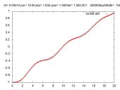
Figure 2: Spring-Block Model, Movement, $h$=0.0001,$\sqrt{k/m}$=10.0, $\eta/m$=1.0, ${\bar{V}}$=1.0, $\bar{\ell}$=1.0, total step no =20000. The step-wise solution (2) correctly reproduces the analytic solution: $x(t)=\mbox{e}^{-\eta^{\prime}t/2}{\bar{V}}\{({\eta^{\prime}}^{2}/2\omega^{2}-1)(\sin\Omega t)/\Omega+(\eta^{\prime}/\omega^{2})\cos\Omega t\}-\bar{\ell}+{\bar{V}}(t-\eta^{\prime}/\omega^{2}){\quad,}\Omega=(1/2)\sqrt{4\omega^{2}-{\eta^{\prime}}^{2}}=9.99{\quad,}\ 0\leq t\leq 2{\quad,}\quad x(0)=-\bar{\ell},\ \dot{x}(0)=0$.

This is the ordinary one for the spring-block model. See Fig.2.

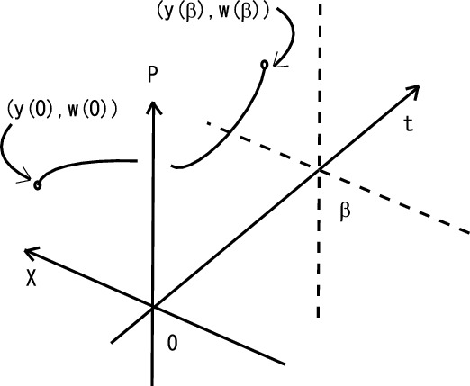
Figure 4: The path $\{(y(t),w(t),t)|0\leq t\leq\beta\}$ of line in 3D bulk space (X,P,t).

The graph of movement (${x_{n}}$, eq.(2)) is shown in Fig.2. From the graph, we see this system starts with the stick-slip motion and reaches the steady state as $n\rightarrow\infty$. Fig.4 shows the energy change as the step flows. It shows the energy oscillates periodically and the amplitude goes down as the step goes. The physical dimensions of the parameters in (3) are listed as

$$[m]=\mbox{M},[k]=\mbox{M}\mbox{T}^{-2},[\bar{\ell}]=\mbox{L},\ [\eta]=\mbox{M}\mbox{T}^{-1},$$

$${[{{\bar{V}}}]}=\mbox{L}\mbox{T}^{-1},$$ (4)

where we assume $[x]=$L, $[t]=$T and $[h]=$T. (M: mass, T: time, L: length.)

Now we consider N copies of the one body system (2). N is sufficiently large, for example, $10^{23}$(1 mol). We are modeling the present statistical system as follows. The N particles are ”moderately” interacting each other in such way that each particle almost independently moves except that energy is exchanged. The interaction is not so strong as to break the dynamics (2). We use Feynman’s path-integral method in order to take the statistical average of this N-copies system. The statistical ensemble measure will be given explicitly.

From the energy expression (1), we can read the metric (geometry) of this mechanical system.

$${\Delta s_{n}}^{2}\equiv 2h^{2}(K_{n}({x_{n}})-K_{n}^{0})$$

$$=2~{}dt^{2}V_{1}({X_{n}})+(\Delta{X_{n}})^{2}+(\Delta{P_{n}})^{2},$$

$$V_{1}({X_{n}})\equiv V(\frac{{X_{n}}}{\sqrt{\eta h}})-nk\sqrt{\frac{h}{\eta}}{\bar{V}}{X_{n}},\ dt\equiv h,$$ (5)

where ${X_{n}}\equiv\sqrt{\eta h}{x_{n}},~{}{P_{n}}/\sqrt{m}\equiv hv_{n}=({x_{n}}-x_{n-1}),$. Using this metric, we can introduce the associated statistical ensemble of the spring-block model[19, 20, 21].

[Statistical Ensemble 1a]

The first choice of the metric in the 3D (t,X,P) manifold is the Dirac-type one:

$$(ds^{2})_{D}\equiv 2V_{1}(X)dt^{2}+dX^{2}+dP^{2}$$

$$-\ \mbox{on-path}~{}(X=y(t),P=w(t))\rightarrow$$

$$(2V_{1}(y)+\dot{y}^{2}+\dot{w}^{2})dt^{2},$$ (6)

where $\{(y(t),w(t))|0\leq t\leq\beta\}$ is a path (line) in the 3D space. See Fig.4. (The momentum variable $P$ is the ”extra” coordinate in the holographic view. ) The length between $0\leq t_{n}=nh\leq\beta$ and the ensemble measure are given by

$$L_{D}=\int_{0}^{\beta}ds|_{on-path}=\int_{0}^{\beta}\sqrt{2V_{1}(y)+\dot{y}^{2}+\dot{w}^{2}}dt$$

$$=h\sum_{n=0}^{\beta/h}\sqrt{2V_{1}(y_{n})+\dot{y}_{n}^{2}+\dot{w}_{n}^{2}},\ d\mu=\mbox{e}^{-{\frac{1}{\alpha}}L_{D}}\prod_{t}{\cal D}y{\cal D}w,$$

$$\mbox{e}^{-\beta F}=\int\prod_{n}dy_{n}dw_{n}\mbox{e}^{-{\frac{1}{\alpha}}L_{D}},$$ (7)

where the free energy $F$ is defined. ($\mbox{e}^{-\beta F}$ is the partition function.) $\alpha$ is a parameter (’string tension’) with the dimension of $\sqrt{M}L/T$. The dimensionless one $\alpha^{\prime}$ can be defined by $\alpha^{\prime}=\alpha/D_{c}$ where $D_{c}$ is the characteristic dimensional unit with the dimension of $\sqrt{M}L/T$. For example $\sqrt{m}\bar{\ell}/h$, $\bar{\ell}\eta/\sqrt{m}$, or $\bar{\ell}\sqrt{k}$. $\alpha^{\prime}$ is determined by the experimental data.

[Statistical Ensemble 1b]

The second choice of the metric is the standard type:

$$(ds^{2})_{S}\equiv\frac{1}{dt^{2}}[(ds^{2})_{D}]^{2}\ \ -\mbox{on-path}\rightarrow$$

$$(2V_{1}(y)+\dot{y}^{2}+\dot{w}^{2})^{2}dt^{2}.$$ (8)

Then the statistical ensemble is given by using the following length:

$$L_{S}=\int_{0}^{\beta}ds|_{on-path}=\int_{0}^{\beta}(2V_{1}(y)+\dot{y}^{2}+\dot{w}^{2})dt=$$

$$h\sum_{n=0}^{\beta/h}(2V_{1}(y_{n})+\dot{y}_{n}^{2}+\dot{w}_{n}^{2}),$$

$$d\mu=\mbox{e}^{-{\frac{1}{\alpha}}L_{S}}{\cal D}y{\cal D}w,\ \mbox{e}^{-\beta F}=\int\prod_{n}dy_{n}dw_{n}\mbox{e}^{-{\frac{1}{\alpha}}L_{S}}$$

$$=(\mbox{const})\int\prod_{n=0}^{\beta/h}dy_{n}\mbox{e}^{-\frac{h}{\alpha}(2V_{1}(y_{n})+\dot{y}_{n}^{2})}.$$ (9)

Note that $w(t)$ decouples from $y(t)$. The last expression is, when ${\bar{V}}=0,\bar{\ell}=0$, the same as the partition function of the system of N($=\beta/h$) harmonic oscillators with the frequency $\sqrt{k/\eta h}$[19]. The minimal path of (9), by changing $y_{n}~{}\rightarrow y,~{}nh~{}\rightarrow t$ and using the variation $y~{}\rightarrow~{}y+\delta y$, we obtain

$$-\eta h\ddot{x}=k({\bar{V}}t-x-\bar{\ell}),\ \ x=\frac{y}{\sqrt{\eta h}}{\quad.}$$ (10)

Comparing with (3), we notice 1) the viscous term disappeared;  2) the mass parameter $m$ is replaced by $\eta h$;  3) the sign in front of the acceleration-term (inertial-term) is different. By changing to the Euclidean time $\tau=it$, the above equation reduces to the harmonic oscillator when we take ${\bar{V}}=0,~{}\bar{\ell}=0$.

[Statistical Ensemble 2]

The first two statistical ensembles are based on the line in the 3D manifold (t,X,P). We present here another type which is based on the surface in the 3D space. First the 3D metric (Dirac type) is re-expressed in the following general form.

$$(ds^{2})_{D}\equiv 2V_{1}(X)dt^{2}+dX^{2}+dP^{2}\equiv e_{1}G_{IJ}({\tilde{X}})d{\tilde{X}}^{I}d{\tilde{X}}^{J},$$

$$I,J=0,1,2;\ ({\tilde{X}}^{0},{\tilde{X}}^{1},{\tilde{X}}^{2})\equiv(t/d_{0},X/d_{1},P/d_{2})$$

$$e_{1}=m\bar{\ell}^{2},\ d_{0}=\sqrt{\frac{k}{m}},d_{1}=d_{2}=\sqrt{m}\bar{\ell},$$

$$(G_{IJ})=\left(\begin{array}[]{ccc}2{d_{0}}^{2}V_{1}(d_{1}{\tilde{X}}^{1})&0&0\\ 0&{d_{1}}^{2}&0\\ 0&0&{d_{2}}^{2},\end{array}\right)$$ (14)

where we have introduced the dimensionless coordinates ${\tilde{X}}^{I}$. Here we introduce the following surface to define a ”path” (surface) in the 3D space.

$$\frac{X^{2}}{{d_{1}}^{2}}+\frac{P^{2}}{{d_{2}}^{2}}=\frac{r(t)^{2}}{{d_{1}}^{2}},\ \ \ 0\leq t\leq\beta,$$ (15)

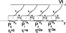
Figure 6: Burridge-Knopoff Model  (23)

where the radius parameter r is chosen to have the dimension of $\sqrt{M}L$. See Fig.6. Then we can define the induced metric $g_{ij}$ on the 2D surface.

$$\left.(ds^{2})_{D}\right|_{\mbox{on-path}}=\left.2V_{1}(X)dt^{2}+dX^{2}+dP^{2}\right|_{\mbox{on-path}}$$

$$=e_{1}\sum_{i,j=1}^{2}g_{ij}({\tilde{X}})d{\tilde{X}}^{i}d{\tilde{X}}^{j}{\quad,}\quad e_{1}=m\bar{\ell}^{2}{\quad,}$$

$$(g_{ij})=\left(\begin{array}[]{cc}1+\frac{e_{1}}{{d_{1}}^{2}}\frac{2V_{1}}{r^{2}\dot{r}^{2}}X^{2}&\frac{e_{1}}{d_{1}d_{2}}\frac{2V_{1}}{r^{2}\dot{r}^{2}}XP\\ \frac{e_{1}}{d_{1}d_{2}}\frac{2V_{1}}{r^{2}\dot{r}^{2}}PX&1+\frac{e_{1}}{{d_{2}}^{2}}\frac{2V_{1}}{r^{2}\dot{r}^{2}}P^{2}\end{array}\right),$$ (18)

Using the (dimensionless) surface area $A$, the third partition function $\mbox{e}^{-\beta F}$ is given by

$$A=\int\sqrt{\det g_{ij}}d^{2}{\tilde{X}}=\frac{1}{d_{1}d_{2}}\int\sqrt{1+\frac{2V_{1}}{\dot{r}^{2}}}dXdP,$$

$$\mbox{e}^{-\beta F}=\int_{0}^{\infty}d\rho\int_{\begin{array}[]{c}r(0)=\rho\\ r(\beta)=\rho\end{array}}\prod_{t}{\cal D}X(t){\cal D}P(t)\mbox{e}^{-\frac{1}{\alpha}A},$$ (21)

where $\alpha$ is the (dimensionless) ”string” constant and here is a model parameter. It is determined by fitting the present result with the experimental data. (Note $\frac{2V_{1}}{\dot{r}^{2}}$ is dimensionless. )

3 BURRIDGE-KNOPOFF MODEL

Let us take the following $n$-th energy function to define Burridge-Knopoff (BK) model in the step($n$) flow method.

$$I_{n}(x)=-xF(\dot{x}_{n-1})+G(\dot{x}_{n-1})\frac{1}{a}(x-x_{n-1})(\dot{x}_{n-1}-\dot{x}_{n-2})$$

$$+\frac{m}{2}(\frac{dx}{dt})^{2}-\frac{k}{2}(x-Vt)^{2}+\frac{K}{2a^{2}}(x-2x_{n-1}+x_{n-2})^{2}+I_{n}^{0},$$ (22)

where $\dot{x}_{n}=d{x_{n}}(t)/dt$. $t$ is the time variable. $I_{n}^{0}$ is a constant term which does not depend on $x(t)$. We consider the system of $N$ particles (blocks) which distribute over the (1-dim) space $\{y\}$. $m$ is the mass of one block. $k$ and $K$ are the spring-constants, the former is for the springs connecting the blocks, the latter is for the springs connecting to the moving (velocity $V$ ) ’plate’. The coordinate $y$ is taken to be periodic: $y\rightarrow y+2L$. The particles (blocks) are moving around the equilibrium points $\{P_{n}~{}|~{}n=1,2,\cdots,N-1,N\}$ where $P_{N}\equiv P_{0}$ (periodic boundary condition). The point $P_{n}$ is located at $y=y_{n}\equiv na$ ($Na=2L$) where $a$ is the ’lattice-spacing’. $N(=2L/a)$ is a huge number and the present system constitutes the statistical ensemble. The n-th particle’s position at $t$, ${x_{n}}(t)$ (deviation from the equilibrium point $P_{n}$) is determined by the energy minimal principle $\delta I_{n}(x)|_{x={x_{n}}}=0$ with the pre-known movement of the (n-1)-th particle, $x_{n-1}(t)$, and that of the (n-2)-th, $x_{n-2}(t)$.

$$-m\frac{d^{2}{x_{n}}}{dt^{2}}-F(\dot{x}_{n-1})+G(\dot{x}_{n-1})~{}\frac{\dot{x}_{n-1}-\dot{x}_{n-2}}{a}$$

$$-k~{}({x_{n}}-Vt)+\frac{K}{a^{2}}~{}(x_{n}-2x_{n-1}+x_{n-2})=0,$$ (23)

where $0\leq t\leq\beta$, and $F(\dot{x}_{n-1})$ and $G(\dot{x}_{n-1})$ are some functions of $\dot{x}_{n-1}$. This recursion relation determines the space-propagation. We assume the system is periodic in time: $t\ \rightarrow\ t+\beta$. This is Burridge-Knopoff model (Fig.6). (See the recent review article ref.[14] for the use of BK model in the earthquake phenomena. ) G is newly introduced in the present paper.

In the continuous space limit:

$$aN=2L\ (\mbox{fixed}),\ a\ \rightarrow\ +0,\ N\ \rightarrow\ \infty,$$

$$y_{n}\ \rightarrow\ y,\ x_{n}\ \rightarrow\ x,\ (x_{n}-x_{n-1})/a\ \rightarrow\ \partial x/\partial y,$$ (24)

the step flow equation (23) reduces to

$$-m\frac{\partial^{2}x}{\partial t^{2}}-F(\dot{x})+G(\dot{x})\frac{\partial^{2}x}{\partial y\partial t}-k(x-Vt)+K\frac{\partial^{2}x}{\partial y^{2}}=0,$$

$$x=x(t,y){\quad,}\quad\dot{x}=\frac{\partial x(t,y)}{\partial t}{\quad.}$$ (25)

Note that, in the third term of the above equation, there appears the velocity-gradient $\frac{\partial^{2}x}{\partial y\partial t}$. (When the system slowly oscillates and G is expanded as $G(\dot{x})=\eta+c_{1}\dot{x}+\cdots$, the first constant is the viscosity. ) The physical dimensions of the parameters in (25) are listed as

$$[m]=\mbox{M},\ [k]=\mbox{M}\mbox{T}^{-2},\ [V]=\mbox{L}\mbox{T}^{-1},\ [K]=\mbox{M}\mbox{L}^{2}\mbox{T}^{-2},$$ (26)

where we assume $[x]=[y]=$L, $[t]=$T and $[a]=$L.

Using the periodicity in time, we can read the metric (geometry) of this mechanical system.

$${\Delta s_{n}}^{2}\equiv 2a^{2}(I_{n}({x_{n}})-I_{n}^{0})=$$

$$\{-2{x_{n}}F(\dot{x}_{n-1})+m{\dot{x}_{n}}^{2}-k({x_{n}}-Vt)^{2}\}dy^{2}$$

$$-a\frac{\partial G(\dot{x}_{n-1})}{\partial t}~{}{\Delta{x_{n}}}^{2}+Ka^{2}~{}{\Delta{\tilde{v}}_{n}}^{2}{\quad,}\quad dy\equiv a,$$

$$\Delta{x_{n}}\equiv{x_{n}}-x_{n-1},\ \frac{{x_{n}}-x_{n-1}}{a}\equiv{\tilde{v}}_{n},\ {\tilde{v}}_{n}-{\tilde{v}}_{n-1}=\Delta{\tilde{v}}_{n},$$ (27)

where we assume $\Delta\dot{x}_{n-1}=\Delta\dot{x}_{n}$. ${\tilde{v}}_{n}$ is the longitudinal strain. The full(complete) metric, $G_{IJ}$, is constructed from (27) as

$${\widetilde{ds}}^{2}=\{-2xF(v)+mv^{2}-k(x-Vt)^{2}\}(dy^{2}-dt^{2})$$

$$+ma^{2}{dv}^{2}-a\frac{\partial G(v)}{\partial t}~{}{dx}^{2}+Ka^{2}~{}(\frac{\partial v}{\partial y})^{2}{dt}^{2}$$

$$=e_{1}G_{IJ}(X)dX^{I}dX^{J},e_{1}=Ka^{2}~{}\mbox{or}~{}ma^{2}V^{2},v\equiv\dot{x}=\frac{\partial x}{\partial t},$$

$$(X^{I})=(X^{0},X^{1},X^{2},X^{3})=(t/d_{0},y/d_{1},x/d_{2},v/d_{3}),$$

$$d_{0}=\sqrt{\frac{m}{k}},d_{1}=V\sqrt{\frac{m}{k}},d_{2}=\sqrt{\frac{K}{k}},d_{3}=\sqrt{\frac{K}{m}},$$ (28)

where we use $d{\tilde{v}}=d(\partial x/\partial y)=(\partial v/\partial y)dt$. $X^{I}$ are the dimensionless coordinates. Note that we have here done the natural replacement: $dy^{2}\ \rightarrow\ -dt^{2}+dy^{2}$ and the addition of $ma^{2}{dv}^{2}$. (For the damped harmonic oscillator limit, $F=G=0,V=K=0,dy=0$, the line element reduces to $-m{dx}^{2}+kx^{2}{dt}^{2}+ma^{2}{dv}^{2}$[19]. ) $G_{IJ}(X)$ is the metric in 4D manifold $(X^{I})$. Note that both $d_{1}$ and $d_{2}$ have the same dimension of Length. $d_{1}$ (large scale) comes from $V$, whereas $d_{2}$ (small scale) from $K$. The 2 coordinates, $y$ and $x$, both describe the position in the space, but their roles are different. In the terminology of the general relativity, the former is the general coordinate and the latter the local coordinate. (The momentum coordinate $X^{3}=v/d_{3}$ is the ”extra” coordinate in the holographic view.)

Now we take the following map from the 2D space $\{(t,y)|~{}0\leq t\leq\beta,~{}0\leq y\leq 2L\}$ to the 4D space $(t,y,x,v)$. (The 4D space is called ”target space” in the string-theory community. )

$$x=\bar{x}(t,y),\ v=\bar{v}(t,y),$$

$$d\bar{x}=\frac{\partial\bar{x}}{\partial t}dt+\frac{\partial\bar{x}}{\partial y}dy,\ d\bar{v}=\frac{\partial\bar{v}}{\partial t}dt+\frac{\partial\bar{v}}{\partial y}dy.$$ (29)

This map expresses a 2D surface in the 4D space (Fig.7). On the surface, the line element (28) reduces to

$${\widetilde{ds}}^{2}\ -\mbox{on surface}\rightarrow\ e_{1}g_{ij}(X)dX^{i}dX^{j},\ \ \ g_{00}=$$

$$\frac{a^{2}}{e_{1}}\left\{-H(\bar{x},\bar{v})+ma^{2}(\frac{\partial\bar{v}}{\partial t})^{2}-\frac{\partial G}{\partial t}(\frac{\partial\bar{x}}{\partial t})^{2}+Ka^{2}(\frac{\partial\bar{v}}{\partial y})^{2}\right\},$$

$$g_{01}=g_{10}=\frac{a^{2}\sqrt{m}}{{e_{1}}^{3/2}}\left\{ma^{2}\frac{\partial\bar{v}}{\partial t}\frac{\partial\bar{v}}{\partial y}-\frac{\partial G}{\partial t}\frac{\partial\bar{x}}{\partial t}\frac{\partial\bar{x}}{\partial y}\right\},$$

$$g_{11}=\frac{a^{2}}{e_{1}}\left\{H(\bar{x},\bar{v})+ma^{2}(\frac{\partial\bar{v}}{\partial y})^{2}-\frac{\partial G}{\partial t}(\frac{\partial\bar{x}}{\partial y})^{2}\right\},$$

$$H(\bar{x},\bar{v})\equiv-2\bar{x}F(\bar{v})+m\bar{v}^{2}-k(\bar{x}-Vt)^{2},$$ (30)

where $\frac{\partial G}{\partial t}=\frac{dG(\bar{v})}{d\bar{v}}\frac{\partial\bar{v}}{\partial t}$ and $i=0,1$. The number of blocks $N$ is a huge number, the present system statistically fluctuates. We regard the ensemble as the collection of possible surfaces $(\bar{x}(t,y),\bar{v}(t,y))$ in the 4D space $(t,y,x,v)$. The probability for each surface (system configuration) is specified by its area $A(\bar{x},\bar{v})$ as follows. Using the (dimensionless) surface area $A$, the partition function $\mbox{e}^{-\beta F}$ is given by

$$A[\bar{x}(t,y),\bar{v}(t,y)]=\frac{1}{d_{0}d_{1}}\int_{0}^{\beta}dt\int_{0}^{2L}dy\sqrt{\det g_{ij}},$$

$$\mbox{e}^{-\beta F}=\int\prod_{t,y}{\cal D}\bar{x}(t,y){\cal D}\bar{v}(t,y)\mbox{e}^{-\frac{1}{\alpha}A},$$ (31)

where $\alpha$ is a dimensionless model parameter. $F$ is the free energy. $\alpha$ is determined by comparing the present result and the experimental data. The minimum area surface, which gives the main contribution to the above quantity, is given by the following equation.

$$\frac{\partial A}{\partial\bar{x}(t,y)}=0\ ,\ \ \frac{\partial A}{\partial\bar{v}(t,y)}=0.$$ (32)

4 CONCLUSION

We have treated two friction models: the spring-block model and Burridge-Knopoff model. Both are simple earthquake models. We have presented how to evaluate the statistical fluctuation effect. It is based on the geometry appearing in the system dynamics. In the text, the metric is obtained in (6) and (8) for the SB model and in (28) for the BK model.

Multiple scales exist in both models. For the SB model, two length scales, one is from the natural length of the string $\bar{\ell}$ and the other from the external velocity ${\bar{V}}$. For the BK model, three length scales exist. The one from the external velocity $V$, that from the spring constant $K$ and the block spacing $a$. As shown in the text, the use of dimensionless quantities clarifies the description. The multiple scales indicate the existence of the fruitful phases in the present statistical systems.

As described in (2) and (23), the dissipative systems are treated by using the minimal principle. The difficulty of the hysteresis effect (non-Markovian effect) [19] is avoided in the present approach. These are the advantage of the discrete Morse flow method. We do not use the ordinary time $t$, instead, exploit the step number $n$ ($t_{n}=nh$).

We have presented several theoretical proposals for the statistical ensembles appearing in the friction phenomena. In order to select which one is the most appropriate, it is necessary to numerically evaluate the models with the proposed ensembles and compare the result with the real data appearing both in the natural phenomena and in the laboratory experiment.

Acknowledgment

The author thanks T. Hatano (Earthquake Research Inst., Univ. of Tokyo) for introducing ref.[14] and the general discussion about earthquake. He also thanks H. Kawamura (Dep. of Earth and Space Science, Osaka Univ.) for the explanation about the numerical simulation of Burridge-Knopoff model.

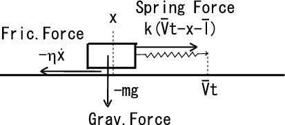
Figure 1: The spring-block model, (3).

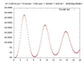
Figure 3: Spring-Block Model, Energy Change, $h$=0.0001,$\sqrt{k/m}$=10.0, $\eta/m$=1.0, ${\bar{V}}$=1.0, $\bar{\ell}$=1.0, total step no =20000.

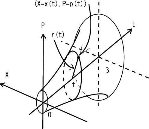
Figure 5: The two dimensional surface, (15), in 3D bulk space (X,P,t).

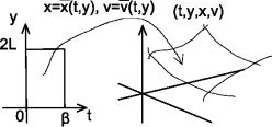
Figure 7: The two dimensional surface, (29), in 4D space (t,y,x,v).