Tuning a magnetic Feshbach resonance with spatially modulated laser light

Abstract

We theoretically investigate the control of a magnetic Feshbach resonance using a bound-to-bound molecular transition driven by spatially modulated laser light. Due to the spatially periodic coupling between the ground and excited molecular states, there exists a band structure of bound states, which can uniquely be characterized by some extra bumps in radio-frequency spectroscopy. With the increasing of coupling strength, the series of bound states will cross zero energy and directly result in a number of scattering resonances, whose position and width can be conveniently tuned by the coupling strength of the laser light and the applied magnetic field (i.e., the detuning of the ground molecular state). In the presence of the modulated laser light, universal two-body bound states near zero-energy threshold still exist. However, compared with the case without modulation, the regime for such universal states is usually small. An unified formula which embodies the influence of the modulated coupling on the resonance width is given. The spatially modulated coupling also implies a local spatially varying interaction between atoms. Our work proposes a practical way of optically controlling interatomic interactions with high spatial resolution and negligible atomic loss.

I Introduction

Ultracold atoms provides an ideal platform to investigate and simulate many-body problems of condensed-matter physics, e.g., the Mott insulator transition Bloch , magnetic phase transition Lewenstein , because of their unprecedented controllability in purity and interatomic interactions. There are a number of tools now available to tune the interatomic interactions, such as magnetic and optical Feshbach resonances, optical lattices, etc.

The magnetic Feshbach resonance - resulting from the hyperfine coupling between two atomic states (i.e., open channel) and a molecular state (closed channel) near zero energy - have been widely used Kohler ; Chin , allowing the realization of the long-sought crossover from a molecular Bose-Einstein condensate (BEC) to a Bardeen-Cooper-Schrieffer (BCS) superfluid and the investigation of interesting few-body physics such as Efimov effects Braaten ; Kraemer .

The interaction between atoms can be also tuned by laser light near photo-association transition, when two free atoms couple to an excited molecular state Fedichev ; Bohn ; Bohn2 . This so-called optical Feshbach resonance has been experimentally realized Fatemi ; Theis . Compared with the magnetic Feshbach resonance, optical Feshbach resonance could be used to control the interatomic interaction with high temporal and spatial flexibility. In addition, the optical transition between atomic states and molecular states is always available for most atomic species. Hence, optical Feshbach resonance becomes crucial to control the interatomic interaction for alkaline-earth atoms because of the lack of magnetic structure in their ground states Ciurylo ; Enomoto ; Thalhammer . In a recent experiment of optical Feshbach resonance, optical standing wave is used to couple atomic and molecular states of ytterbium-174 atoms, leading to a spatially modulated interaction between atoms Yamazaki . Theoretically, this spatially modulated interatomic interaction was understood by using a two-channel model Qi . Future experiments on, e.g., the simulation of Hawking radiation in cold atoms Garay ; Carusotto , the emission of solitons Rodas-Verde , the dynamics of BEC collapse Dong ; Yan , the localized to delocalized transition of solitons Abdullaev , and the phase separation of Bose and Fermi gases Chien , all resulting from spatially varying interactions, may benefit from the control of interatomic interactions with high spatial and temporal resolutions.

However, due to the large light-induced atomic loss, the use of optical Feshbach resonance is greatly limited. To reduce the loss, it has been proposed to use alkaline-earth atoms with narrow inter-combination line-width Blatt . Alternatively, one may optically control a magnetic Feshbach resonance by using a bound-to-bound transition between two molecular states Bauer ; Bauer2 ; Fu or by using a molecular dark state Wu . Experimentally, the shift of the magnetic Feshbach resonance position and the modification of the two-body $s$-wave scattering length due to the bound-to-bound transition have been demonstrated for both atomic Bose Bauer ; Bauer2 and Fermi gases Fu , by using spatially uniform laser light.

In this work, we investigate the optical control of a magnetic Feshbach resonance by using spatially varying (i.e., standing-wave-like) laser light, which drives the bound-to-bound transition between a ground molecular state and an excited molecular state. This scheme can directly be implemented in current experiments Bauer ; Fu by replacing the uniform laser light with a standing-wave light. It offers the ability to tune the interatomic interactions with a spatial modulation at the sub-micron level. Compared with the previous spatial modulation of interatomic interactions with optical Feshbach resonance Yamazaki ; Qi , the major advantage of our scheme is that the optical induced atomic loss would be significantly suppressed Bauer ; Fu . As a result, our proposal provides a practical way to experimentally realize spatially modulated interatomic interactions, for the purpose of simulating related many-body problems. As we shall see, our scheme also has the advantage of tuning the width of Feshbach resonances, with a great flexibility.

The rest of paper is organized as follows. In the next section (Sec. II), we introduce the model Hamiltonian and calculate the energy bands of bound states. The scattering states are also investigated and a series of scattering resonances are obtained. In Sec. III, we present a detailed analysis and discussion to our results. Sec. IV is devoted to a summary of this work.

II Theoretical framework

II.1 Model Hamiltonian

In the absence of the bound-to-bound molecular transition, the system can be described by the following atom-molecule Hamiltonian Drummond ; Timmermans ; Timmermans2 ; Holland ,

$$H =H_{0a}+H_{Ia}+H_{g}+H_{ag},$$ (1)

$$H_{0a} =\sum_{\sigma}\int d\vec{r}\psi_{\sigma}^{\dagger}(\vec{r})\left[-\frac{\hbar^{2}\nabla^{2}}{2m}-\mu\right]\psi_{\sigma}(\vec{r}),$$

$$H_{Ia} =U\int d\vec{r}\psi_{\uparrow}^{\dagger}(\vec{r})\psi_{\downarrow}^{\dagger}(\vec{r})\psi_{\downarrow}(\vec{r})\psi_{\uparrow}(\vec{r}),$$

$$H_{g} =\int d\vec{R}\phi^{\dagger}(\vec{R})\left[-\frac{\hbar^{2}\nabla^{2}}{2M}-2\mu+v_{g}\right]\phi(\vec{R}),$$

$$H_{ag} =\chi\int d\vec{R}\left[\phi^{\dagger}(\vec{R})\psi_{\uparrow}(\vec{R}/2)\psi_{\downarrow}(\vec{R}/2)+\textrm{H.c.}\right],$$

where $H_{0a}$ and $H_{Ia}$ are respectively the kinetic Hamiltonian and interaction Hamiltonian of atoms with the field operator $\psi_{\sigma}(\vec{r})$ ($\sigma=\uparrow,\downarrow$); $H_{g}$ is the Hamiltonian of molecules in their ground state with the field operator $\phi(\vec{R})$ and $v_{g}$ denotes the energy difference between the molecular state and atomic state; $H_{ag}$ describes the atom-molecule coupling and models the conversion between atoms and molecules. The mass of molecules is twice of atomic mass $M=2m$. $\mu$ is the chemical potential. H.c. denotes the Hermitian conjugate. Note that we have assumed short-range contact interactions for both interatomic interaction $U(\vec{r}-\vec{r}^{\prime})=U\delta(\vec{r}-\vec{r}^{\prime})$ and atom-molecule coupling $\chi(\vec{R};\vec{r},\vec{r}^{\prime})=\chi\delta[\vec{R}-(\vec{r}+\vec{r}^{\prime})/2]\delta(\vec{r}-\vec{r}^{\prime})$.

We now consider the molecular bound-bound transition driven by a standing-wave laser light $\Omega\cos(\vec{K}\cdot\vec{R})/2$, where $\Omega$ is the related Rabi frequency and $\vec{K}$ is the wave-vector of the light. By using the field operator $\phi_{e}(\vec{R})$ for the excited molecular state and taking the rotating-wave approximation, we obtain the following two additional terms Bauer ; Fu :

$$H_{e} = \int d\vec{R}\phi_{e}^{\dagger}(\vec{R})\left[-\frac{\hbar^{2}\nabla^{2}}{2M}-2\mu+v_{e}-\Delta-i\frac{\gamma}{2}\right]\phi_{e}(\vec{R}),$$

$$H_{ge} = \int d\vec{R}\frac{\Omega\cos(KX)}{2}\left[\phi^{\dagger}(\vec{R})\phi_{e}(\vec{R})+\phi_{e}^{\dagger}(\vec{R})\phi(\vec{R})\right],$$ (2)

where $H_{e}$ is the kinetic Hamiltonian of the excited molecular state, $v_{e}$ is the energy of the excited state relative to the atomic state, $\Delta$ is the detuning of the molecular transition, $\gamma$ describes the decay of the excited state, and $H_{ge}$ is the coupling between the ground and excited states through the optical standing wave. We have assumed that the laser light is applied along the $x$-direction so that $\cos(\vec{K}\cdot\vec{R})=\cos(KX)$.

In the case of large detuning ($\Delta\gg v_{e}$, $\gamma$), we may safely neglect the decay of the excited molecular state (i.e., $\gamma=0$) and eliminate the field operator $\phi_{e}(\vec{R})$. The coupling ($H_{ge}$) between molecular states leads to a Stark energy shift $\Omega^{2}\cos^{2}(KX)/(4\Delta)$ for the molecular ground state and consequently we have a modified Hamiltonian for ground-state molecules,

$$\tilde{H}_{g} =\int d\vec{R}\phi^{\dagger}\left[-\frac{\hbar^{2}\nabla^{2}}{2M}-2\mu+v_{g}+\frac{\Omega^{2}\cos{}^{2}(KX)}{4\Delta}\right]\phi(\vec{R}).$$ (3)

It is obvious that the Stark energy shift plays the role of optical lattices for ground-state molecules Fedichev2 ; Orso . By taking a Fourier transformation, the total Hamiltonian can be rewritten in momentum space as

$$H = H_{0a}+H_{Ia}+\tilde{H}_{g}+H_{ag},$$

$$H_{0a} = \sum_{\vec{k}\sigma}(\epsilon_{\vec{k}}-\mu)C_{\vec{k}\sigma}^{\dagger}C_{\vec{k}\sigma},$$

$$H_{Ia} = U\sum_{\vec{k},\vec{k}^{\prime},\vec{q}}C_{\vec{q}/2+\vec{k},\uparrow}^{\dagger}C_{\vec{q}/2-\vec{k},\downarrow}^{\dagger}C_{\vec{q}/2-\vec{k}^{\prime},\downarrow}C_{\vec{q}/2+\vec{k}^{\prime},\uparrow},$$

$$\tilde{H}_{g} = \sum_{\vec{q}}\left(\frac{\epsilon_{\vec{q}}}{2}-2\mu+v_{g}+\frac{\Omega^{2}}{8\Delta}\right)b_{\vec{q}}^{+}b_{\vec{q}}$$

$$-\sum_{\vec{q}}\frac{\Omega^{2}}{16\Delta}\left(b_{\vec{q}}^{\dagger}b_{\vec{q}+2K}+\textrm{H.c.}\right),$$

$$H_{ag} = \chi\sum_{\vec{k},\vec{q}}\left(b_{\vec{q}}^{\dagger}C_{\vec{q}/2-\vec{k},\downarrow}C_{\vec{q}/2+\vec{k},\uparrow}+\textrm{H.c.}\right).$$ (4)

Here $\epsilon_{\vec{k}}=\vec{k}^{2}/2$ is the kinetic energy (in the units of $m=1$ and $\hbar=1$). The above Hamiltonian will be our starting point. In the following, we will solve the two-particle problem of the Hamiltonian.

Note that, in the case of large detuning, the molecular excited state $|e\rangle$ does not appear in the above Hamiltonian. Note also that, here the lattice potential only appears for the ground molecular state, unlike the case of an optical Feshbach resonance, where the spatial modulation appears in the atom-molecule coupling $\chi$ Qi .

II.2 Two-body bound states

Here we focus on the two-body problem, so the chemical potential $\mu=0$. Due to the presence of the lattice potential, eigenstates can be classified according to quasi-momentum $q\in[-K,K]$ (Note that the period of the lattice in Eq. (3) is half of the wave length of laser beam). Hereafter, $q$ and $K$ are understood as along the $x$-direction unless explicitly specified. It is expected that the eigen-energy would form a band structure. The two-body wave function can be written as

$$|\psi\rangle =\sum_{n}A_{n}|nK+q,g\rangle$$

$$+\sum_{n\vec{k}}B_{n,\vec{k}}|(nK+q)/2+\vec{k},\uparrow;(nK+q)/2-\vec{k},\downarrow\rangle,$$ (5)

where $|nK+q,g\rangle$ is the molecular state with a center-of-mass momentum $nK+q$, $|(nK+q)/2+\vec{k},\uparrow;(nK+q)/2-\vec{k},\downarrow\rangle$ is the state of a pair of atoms with total momentum $nK+q$ and relative momentum $\vec{k}$ and with un-like spins. The two-particle Schrödinger equation reads

$$H|\psi\rangle=E|\psi\rangle,$$ (6)

from which we determine coupled equations for the coefficients $A_{n}$ and $B_{n,k}$,

$$EA_{n} = \left[\epsilon_{nK+q,g}+v_{g}+\frac{\Omega^{2}}{8\Delta}\right]A_{n}$$

$$-\frac{\Omega^{2}}{16\Delta}\left[A_{n+2}+A_{n-2}\right]+\chi\sum_{\vec{k}}B_{n,\vec{k}},$$

$$EB_{n,\vec{k}} = \left[\epsilon_{(nK+q)/2-\vec{k},a}+\epsilon_{(nK+q)/2+\vec{k},a}\right]B_{n,\vec{k}}$$ (7)

$$+U\sum_{\vec{k}^{\prime}}B_{n\vec{k}^{\prime}}+\chi A_{n},$$

where the molecular kinetic energy $\epsilon_{nK+q,g}=(nK+q)^{2}/4$ and the atomic kinetic energy $\epsilon_{(nK+q)/2\pm\vec{k},a}=[(nK+q)/2\pm\vec{k}]^{2}/2$. The above equation demonstrates that the molecular amplitudes of different momenta $A_{n}$ are coupled by the lattice potential. After eliminating the atomic amplitude $B_{n,\vec{k}}$, we obtain,

$$EA_{n} = \left[\epsilon_{nK+q,g}+v_{g}+Z_{n}+\frac{\Omega^{2}}{8\Delta}\right]A_{n}$$ (8)

$$-\frac{\Omega^{2}}{16\Delta}[A_{n+2}+A_{n-2}],$$

where,

$$Z_{n}=\frac{\chi^{2}f_{n}}{1-Uf_{n}},$$

$$f_{n}=\Sigma_{\vec{k}}\frac{1}{E-(\epsilon_{(nK+q)/2-\vec{k},a}+\epsilon_{(nK+q)/2+\vec{k},a})}.$$

The bare parameters ($\chi$, $U$ and $v_{g}$) need to be renormalized to real physical observables Fu , for example,

$$v_{g}+Z_{n}\rightarrow v_{g0}+Z_{n0}=v_{g0}+\frac{\chi_{0}^{2}f_{n0}}{1-U_{0}f_{n0}},$$ (9)

where

$$f_{n0} =\sum_{\vec{k}}\left[\frac{1}{E-[\epsilon_{(nK+q)/2-\vec{k},a}+\epsilon_{(nK+q)/2+\vec{k},a}]}+\frac{1}{\vec{k}^{2}}\right]$$

$$=\sum_{\vec{k}}\left[\frac{1}{E-[(nK+q)^{2}/4+\vec{k}^{2}]}+\frac{1}{\vec{k}^{2}}\right]$$

$$=\frac{\sqrt{-E+(nK+q)^{2}/4}}{4\pi}.$$

Detailed expressions for real observables $v_{g0}$, $\chi_{0}$ and $U_{0}$ are given in the next section.

Eq. (8) differs from the usual eigenvalue problems in that the eigenvalue $E$ appears on both sides of the equation. We can divide the eigenvalue $E$ on both sides of the equation and obtain,

$$A_{n}= \frac{\left[\epsilon_{nK+q,g}+v_{g0}+Z_{n0}+\Omega^{2}/(8\Delta)\right]}{E}A_{n}$$

$$-\frac{\Omega^{2}}{16\Delta E}\left[A_{n+2}+A_{n-2}\right].$$ (10)

The above equation has the form,

$$|\psi\rangle=K(E)|\psi\rangle,$$ (11)

where the matrix elements of the kernel $K(E)$ depend on the eigenvalue $E$. By adjusting $E$ to force the eigenvalues of the kernel $K(E)$ to be 1, we can solve all the eigenvalues and eigenvectors numerically. Then, from the molecular amplitudes ($A_{n}$), one can obtain the atomic amplitudes

$$B_{n,\vec{k}}=\frac{\beta_{n}}{-E_{b}-[\epsilon_{(nK+q)/2-\vec{k},a}+\epsilon_{(nK+q)/2+\vec{k},a}]},$$

where $E_{b}\equiv-E>0$ is the binding energy of the bound state and

$$\beta_{n}\equiv\frac{U_{0}\chi_{0}f_{n0}A_{n}}{1-U_{0}f_{n0}}+\chi_{0}A_{n}.$$ (12)

II.3 Radio-frequency spectroscopy of two-particle bound states

The existence of two-particle bound states may be detected by the radio-frequency (rf) spectroscopy technique. The Hamiltonian of the rf process can be written as Chin2 ; Bartenstein ; Hu

$$V_{rf} =V_{0}\int d\vec{r}\left[\psi_{3}^{\dagger}(\vec{r})\psi_{\downarrow}(\vec{r})+\textrm{H.c.}\right],$$

$$=V_{0}\sum_{\vec{q}}\left[C_{\vec{q},3}^{\dagger}C_{\vec{q},\downarrow}+\textrm{H.c.}\right].$$ (13)

It represents a transition process, where the atoms in the state $|\vec{q},\downarrow\rangle$ are transferred to a third, unoccupied state $|\vec{q},3\rangle$.

Recall that the atomic part of the wave function of a two-particle bound state is given by,

$$|\psi,a\rangle =\sum_{n\vec{k}}B_{n,\vec{k}}|(nK+q)/2+\vec{k},\uparrow;(nK+q)/2-\vec{k},\downarrow\rangle.$$ (14)

By acting $V_{rf}$ on this wave function, we obtain,

$$V_{rf}|\psi,a\rangle$$

$$=-V_{0}\sum_{n\vec{k}\vec{q}^{\prime}}B_{n\vec{k}}C_{\vec{q}^{\prime},3}^{\dagger}C_{(nK+q)/2+\vec{k},\uparrow}^{\dagger}C_{\vec{q}^{\prime},\downarrow}C_{(nK+q)/2-\vec{k},\downarrow}^{\dagger}|0\rangle,$$

$$=-V_{0}\sum_{n\vec{k}}B_{n\vec{k}}C_{(nK+q)/2-\vec{k},3}^{\dagger}C_{(nK+q)/2+\vec{k},\uparrow}^{\dagger}|0\rangle,$$ (15)

which give us the final two-particle state after the rf pulse. Using Fermi’s Golden Rule, the transfer strength of the rf process is given by the following Frank-Condon factor,

$$\Gamma(\omega) =\frac{1}{\mathcal{C}}\sum_{n,\vec{k}}|B_{n,\vec{k}}|^{2}\delta\left(\omega-\left[\frac{(nK+q)^{2}}{4}+\vec{k}^{2}+E_{b}\right]\right),$$ (16)

where the $\delta$-function guarantees energy conservation during the rf process and $\mathcal{C}=\sum_{n,\vec{k}}|B_{n,\vec{k}}|^{2}$ is the normalization constant. By introducing $E_{n}=E_{b}+(nK+q)^{2}/4$, we find that $f_{n0}=\sqrt{E_{b}+(nK+q)^{2}/4}/4\pi=\sqrt{E_{n}}/4\pi$, $|B_{n\vec{k}}|^{2}=\beta_{n}^{2}/(E_{n}+\vec{k}^{2})^{2}$, and $\mathcal{C}=\sum_{n}\beta_{n}^{2}/[8\pi\sqrt{E_{n}}]$. The Frank-Condon factor can then be rewritten as,

$$\Gamma(\omega)=\sum_{n}\frac{\beta_{n}^{2}}{4\pi^{2}\mathcal{C}}\frac{\sqrt{\omega-E_{n}}}{\omega^{2}}\theta(\omega-E_{n}),$$ (17)

where $\theta(x)$ is the Heaviside step function. Therefore, once we obtain $E_{b}$ and $A_{n}$, the rf transfer strength can be calculated straightforwardly.

II.4 Two-particle scattering states

We now consider the low-energy scattering state with energy $E>0$ and $E\ll K^{2}$. Here we focus on the isotropic $s$-wave scattering at the quasi-momentum $q=0$. Without loss of generality, we assume that the incident wave propagates along the $z$-direction. The scattering wave function can be written as

$$|\psi\rangle = |k_{z},\uparrow;-k_{z},\downarrow\rangle+\sum_{n}A_{n}|nK,g\rangle+$$ (18)

$$+\sum_{n,\vec{k}}B_{n,\vec{k}}|nK/2+\vec{k},\uparrow;nK/2-\vec{k},\downarrow\rangle,$$

where the first term on the right-hand side $|k_{z},\uparrow;-k_{z},\downarrow\rangle$ stands for the incident state of two atoms with the total momentum $0$, relative momentum $k_{z}$ and energy $E=k_{z}^{2}$. By substituting the wave function into the two-particle Schrödinger equation, we obtain,

$$EA_{n} = \left[\epsilon_{nK,g}+v_{g}+\frac{\Omega^{2}}{8\Delta}\right]A_{n}-\frac{\Omega^{2}}{16\Delta}\left[A_{n+2}+A_{n-2}\right]$$

$$+\chi\sum_{\vec{k}}B_{m,\vec{k}},$$

$$EB_{n,\vec{k}} = \left[\epsilon_{nK/2-\vec{k},a}+\epsilon_{nK/2+\vec{k},a}\right]B_{n,\vec{k}}$$ (19)

$$+U\sum_{\vec{k}^{\prime}}B_{n\vec{k}^{\prime}}+\chi A_{n}+U\delta_{n,0}.$$

Here, compared with Eq. (7), the extra term $U\delta_{n,0}$ in the last line comes from the incident state with zero total momentum.

It is important to note that, traditionally, in the absence of optical lattices the atomic and molecular states are referred to as the open and closed channels, respectively. In our case with the lattice potential, this two-channel viewpoint should be generalized, as the dispersion relation is now folded into discrete energy bands (i.e., different $n$). That is, we may classify any atomic states with a nonzero band index $n\neq 0$ as a closed channel Qi . As a result, with the lattice potential we are now dealing with a multi-channel scattering problem, instead of the usual two-channel problem. As we shall see later, this multi-channel viewpoint is crucial to understand the width of scattering resonances.

By adopting the similar strategy of eliminating the atomic amplitudes $B_{n,\vec{k}}$ as in the bound state calculation, we obtain,

$$EA_{n} = \left[\epsilon_{nK,g}+v_{g}+Z_{n}+\frac{\Omega^{2}}{8\Delta}\right]A_{n}$$ (20)

$$-\frac{\Omega^{2}}{16\Delta}\left[A_{n+2}+A_{n-2}\right]+\frac{Z_{n}U}{\chi}\delta_{n,0},$$

After the renormalization, the equation becomes

$$EA_{n} =\left[\epsilon_{nK,g}+v_{g0}+Z_{n0}+\frac{\Omega^{2}}{8\Delta}\right]A_{n}$$ (21)

$$-\frac{\Omega^{2}}{16\Delta}\left[A_{n+2}+A_{n-2}\right]+\left(\frac{Z_{n0}U_{0}}{\chi_{0}}+\chi_{0}\right)\delta_{n,0}.$$

We can solve the above linear equation to obtain the molecular amplitudes $A_{n}$, and then the atomic amplitudes $B_{nk}$ through the expression $B_{nk}=\beta_{n}^{\prime}/[-(E_{n}^{\prime}+\vec{k}^{2})]$, where $E_{n}^{\prime}=-E+(nK)^{2}/4$ and

$$\beta_{n}^{\prime}=\frac{U_{0}^{2}f_{n0}\delta_{n,0}+U_{0}x_{0}f_{n0}A_{n}}{1-U_{0}f_{n0}}+x_{0}A_{n}+U_{0}\delta_{n,0}.$$ (22)

II.5 Spatially modulated interatomic interactions

In coordinate space, the atomic part of the scattering wave function can be written as,

$$\langle r|\psi,a\rangle =e^{ik_{z}z}+\sum_{n,\vec{k}}B_{n,\vec{k}}e^{inKX+i\vec{k}\vec{r}},$$

$$=e^{ik_{z}z}+\sum_{n}\frac{1}{(2\pi)^{3}}\int d^{3}\vec{k}\frac{-\beta^{\prime}_{n}}{E^{\prime}_{n}+\vec{k}^{2}}e^{inKX+i\vec{k}\vec{r}},$$

$$=e^{ik_{z}z}-\frac{\beta_{0}^{\prime}e^{i\sqrt{E}r}}{4\pi r}+\sum_{n\neq 0}-\frac{\beta_{n}^{\prime}e^{inKX}e^{-\sqrt{E_{n}^{\prime}}r}}{4\pi r}.$$ (23)

We can see that the wave functions of closed channels ($n\neq 0$) all exponentially decrease with increasing $r$. As the incident energy $E\rightarrow 0$, the $s$-wave scattering amplitude is given by $f_{0}=-\beta_{0}^{\prime}/4\pi$, from which we determine the $s$-wave scattering length

$$a_{eff}=-f_{0}=\frac{\beta_{0}^{\prime}}{4\pi}.$$ (24)

On the other hand, at the short range ($r\rightarrow 0$), the atomic part of the scattering wave function can be expressed as

$$\langle r|\psi,a\rangle \propto 1/r-1/a_{loc}(X)+o(r),$$ (25)

where $o(r)$ represents a quantity at the same order of magnitude of $r$, and $a_{loc}(X)$ can be interpreted as the local $s$-wave scattering length. Comparing Eq. (23) with Eq. (25), we obtain the expression of the local $s$-wave scattering length Qi

$$a_{loc}(X) =\frac{1-\sum_{n\neq 0}U_{n}\cos(nKX)/U_{0}}{1/a_{eff}-\sum_{n\neq 0}U_{n}|n|K\cos(nKX)/U_{0}},$$ (26)

where

$$U_{0} = +\frac{\beta_{0}^{\prime}}{4\pi},$$

$$U_{n} = -\frac{\beta_{n}^{\prime}}{4\pi}.$$ (27)

Note that, when we construct an effective many-body Hamiltonian of our system, the interaction Hamiltonian may be modeled by using the local scattering length $a_{loc}(X)$ Qi , which is position dependent. Thereby, the lattice potential gives rise to a spatially modulated interatomic interaction.

III Results and discussion

Taking an ultracold Fermi gas of ⁴⁰K atoms as an example Fu , at the magnetic Feshbach resonance $B_{0}=202.20\pm 0.02$ G the background scattering length $a_{bg}\simeq 174a_{B}$ ($a_{B}$ is the Bohr radius), the difference in magnetic momentum of atoms and of ground-state molecules is $\mu_{ag}=2\mu_{a}-\mu_{g}\simeq 2\mu_{B}$ ($\mu_{B}$ is the Bohr magneton), and the width of resonance $W\simeq 7.04\pm 0.10$ G. In the following calculations, we take the natural units: the mass of atoms $m=1$, the background scattering length $a_{bg}=1$ and $\hbar=1$. Therefore, energy is measured in units of $\hbar^{2}/ma_{bg}^{2}$. We take the parameters: $B-B_{0}=-0.6$ G; $\Omega=2\pi\hbar\times 0.07$ GHz; the wave length of laser $\lambda=780$ nm; the wave vector $K=2\pi/\lambda$. The physical observables mentioned earlier are related to the above experimental parameters by the expressions,

$$U_{0} = 4\pi\hbar^{2}a_{bg}/m,$$

$$\chi_{0} = 2\hbar\sqrt{\pi a_{bg}W\mu_{ag}/m},$$

$$\nu_{g0} = \mu_{ag}(B-B_{0}).$$ (28)

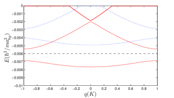
Figure 1: (Color online). The bound states energy spectrum with optical coupling $\Omega^{2}/16\Delta=0.0342$ (dotted blue lines) and $-0.0342$ (solid red lines), respectively. The dashed line indicates the lowest energy of bound states without lattice potential (i.e., $\Omega^{2}/16\Delta=0$).

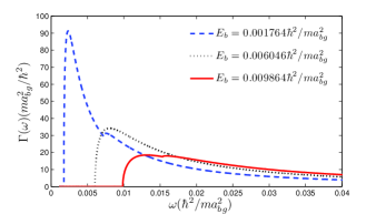
Figure 2: (Color online). The Frank-Condon factor. The dashed blue, dotted black and solid red lines in Fig. 2 correspond bound states 1, 2 and 3 in Fig. 3 (a), respectively [see the three bound states denoted by arrow heads on the rightmost line of the panel (a) of Fig. 3].

In Fig. 1 we show the bound state energies. The dotted blue and solid red lines correspond to the blue ($\Delta>0$) and red detunings ($\Delta<0$), respectively. As anticipated, overall the red detuning gives rise to a lower energy for two-particle bound states. Fig. 2 reports the rf spectroscopy of three lowest bound states located at quasi-momentum $q=0$ for different lattice depths. We find that the smaller binding energy is, the sharper is rf signal (see the dashed blue line in Fig. 2). This is because when the binding energy approach zero, the wave function of bound states extends widely in coordinate space. Accordingly, the wave function in momentum space will concentrate near zero-momentum. So the overlap of wave functions which gives the Frank-Condon factor reaches large value near zero-energy. Due to the coupling of different total momenta, for each bound state its atomic part of the wave-function is a linear superposition of different components with different total momenta, as shown in Eq. (5). This results in additional bumps in the rf spectroscopy, see for example, Eq. (17). Therefore, we may identify the bumps as a unique characteristic of the energy band structure due to the lattice potential. With increasing the lattice potential strength, the bumps becomes more evident. The result of Fig. 2 can be directly verified in current cold-atom experiments by using rf-spectroscopy Bartenstein ; Fu .

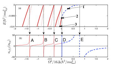
Figure 3: (Color online). The bound states and their corresponding Feshbach resonances at the quasi-momentum $q=0$. The panel (a) gives the evolution of bound state energies with increasing the lattice depth. The panel (b) shows the $s$-wave scattering length ($a_{eff}$). The solid red (dashed blue) lines correspond to the case of $\Delta<0$ ($\Delta>0$). In (a), the dotted lines show the energy branches that do not induce resonance when they cross zero-energy.

To show the evolution of the energy band structure as a function of the lattice depth $\Omega^{2}/16\Delta$, we report $E(q=0)$ in Fig. 3. With increasing the lattice depth, in the case of red detuning ($\Delta<0$), more bound states emerge [see the panel (a) of Fig. 3], while in the case of blue detuning ($\Delta>0$), the energy of bound states move upward and crosses zero-energy. The corresponding evolution of the $s$-wave scattering length is shown in the panel (b) of Fig. 3. A resonance occurs in the $s$-wave scattering length when the energy of bound state crosses zero-energy, as one may anticipate. However, not all the energy branches induce resonance when they cross zero-energy. In the panel (a), the wave function of the bound states shown in dotted red lines is antisymmetric with respect to the momentum $nK=0$ (i.e., $\beta_{n}^{\prime}=-\beta_{-n}^{\prime}$), implying $\beta_{0}^{\prime}=0$. As a result, the $s$-wave scattering length $a_{eff}=\beta_{0}^{\prime}/4\pi=0$ and hence these bound states do not result in any Feshbach resonance. We note that, the resonance induced by a spatially modulated atom-molecule coupling has been previously discussed in the case of optical Feshbach resonance Qi . The appearance of a resonance was similarly found to depend on the symmetry of the bound state.

No.	A	B	C	D	E
$(\Omega^{2}/16\Delta)_{0}$	$-1.385$	$-0.78$	$-0.3279$	$0.01399$	$0.7807$
$W$	$0.3526$	$0.2535$	$0.1403$	$0.0045$	$10.4948$
$E_{\text{uni}}$	$5.1*10^{-5}$	$3.3*10^{-5}$	$1.1*10^{-5}$	$7.6*10^{-9}$	$0.0046$

Table 1: The resonance position and width of the five Feshbach resonances shown in the panel (b) of Fig. 3(in units of $\hbar^{2}/ma_{bg}^{2}$). $E_{\text{uni}}$ is an energy scale associated with the regime for universal two-body bound states (see Eq. (A.13) in the Appendex)

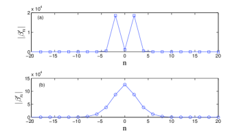
Figure 4: (Color online). The atomic amplitudes as a function of the band index $n$ near the Feshbach resonances D and E (corresponding to the two resonances with blue detuning in the panel (b) of Fig. 3). From the upper panel (a) for the resonance D, we see that the closed channels ($n=\pm 2$) have the largest amplitudes. Therefore, we interpret the resonance D as a closed-channel-dominated resonance. On the contrary, the lower panel (b) for the resonance E corresponds to a entrance-channel-dominated resonance.

Different from the case of optical Feshbach resonance Qi , however, in our case the width of the spatial-modulation-induced resonance varies significantly by changing the depth of the optical lattice potential. Near resonance, the scattering length can be written as

$$a_{eff}=a_{bg}\left[1-\frac{W}{(\Omega^{2}/16\Delta)-(\Omega^{2}/16\Delta)_{0}}\right],$$ (29)

here [$(\Omega^{2}/16\Delta)_{0}$] and ($W$) are the resonance position and width. In Table I, we calculate the width of the five Feshbach resonances shown in the panel (b) of Fig. 3 (for details see Appendix). The position of resonance can be obtained through fitting our numerical data. Generally, the widths of Feshbach resonance are influenced greatly by the other atomic closed channels (see Table. I). In the absence of optical lattice potential, the resonance width of ⁴⁰K atoms near the magnetic field $B_{0}=202.20\pm 0.02$ is about $W\sim 3.3$, in the energy unit of $\hbar^{2}/ma_{bg}^{2}$. From Table. I, we find that, in the presence of the lattice potential, the resonance width can be one order of magnitude larger or smaller than that without the lattice potential. For large blue detuning, the width of resonance E is extremely large. For red detuning we find that the width becomes larger with increasing the depth of the optical coupling $|\Omega^{2}/\Delta|$. As a result, we can access very wide Feshbach resonance by choosing the zero-energy bound state at large lattice depth.

Fig. 4 reports the atomic amplitude $\left|\beta_{n}^{\prime}\right|$ near the Feshbach resonance D and E [see the panel (b) of Fig. 3]. The width of the resonance D is very small. It is a closed-channel-dominated resonance, in the sense that the atomic amplitudes of closed channels $\beta_{n=\pm 2}^{\prime}$ take the largest value relative to the open channel ($\beta_{n=0}^{\prime}$) [see Fig. 4(a)]. On the contrary, the resonance E has a very large resonance width and the atomic amplitude peaks at $n=0$.

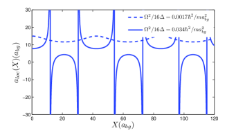
Figure 5: (Color online). The local $s$-wave scattering length near the resonance D. The solid and dashed lines have the scattering length $a_{eff}=12.88a_{bg}$ and $a_{eff}=12.81a_{bg}$, respectively.

It is worth noting that although there is a modulated lattice, universal two-body bound states near zero-energy threshold still exist (see Appendix), whose energy is approximately $E\propto-1/a^{2}_{eff}$. However, the universal regime may be extremely small because of the influence of other atomic closed channels. In Table. I, we calculate an characteristic energy scale $E_{\text{uni}}$ for each resonance, which determines the size of the universal regime. Only when the energy satisfy $|E|\ll E_{\text{uni}}$, the universal expression $E\propto-1/a^{2}_{eff}$ is valid (see Appendix). From Table. I, we find that the universal regimes for Feshbach resonances A, B, C and D are all extremely small. This explains why we can not see the universal behavior from Fig. 3. However, the Feshbach resonance E has a relatively large universal regime compared with others. As a result, the corresponding energy curve looks like quadratic parabola near the Feshbach resonance E.

Fig. 5 shows the spatial dependence of the local $s$-wave scattering length. It is easy to see that the variation period of the scattering length $a_{loc}(X)$ is directly determined by the optical lattice potential. For a weak lattice potential (dashed line), the variation of the local scattering length follows a cosine function. The mean value of the local scattering length is roughly equal to the $s$-wave scattering length $a_{eff}$. For a stronger lattice potential (solid line), although $a_{eff}$ is nearly the same, the value of the local scattering length changes drastically, from positive to negative, when the position $X$ changes. This implies that a reasonably large lattice potential has crucial effects on spatially modulated interatomic interactions, similar to what has already been seen in the case of an optical Feshbach resonance Qi

IV summary

In conclusion, we have investigated how to tune a magnetic Feshbach resonance by using standing-wave laser light that drives a molecular bound-to-bound transition. The two-particle bound states and scattering states (or scattering lengths) are significantly affected by the standing-wave light. A band structure is formed and a series of zero-energy scattering states appear. As a result, a number of laser-induced Feshbach resonances emerge, whose position and width can be tuned by changing the depth of the standing-wave laser. The resulting $s$-wave scattering length near resonance shows a strong spatial dependence. This provides a new tool to control interatomic interactions and therefore opens a new route to study many interesting many-body physics, for example, the exotic soliton, spatially inhomogeneous BCS superfluidity or BEC-BCS crossover, self-trapping of BECs induced by spatially modulated interatomic interactions.

Our proposed scheme can be directly examined in current experiments for an ultracold Fermi gas of ⁴⁰K atoms. Indeed, the optical control of the interaction between ⁴⁰K atoms near the broad Feshbach resonance $B_{0}=202.20\pm 0.02$ has recently been demonstrated Fu , by using a spatially homogeneous laser. Our scheme is straightforward to implement by replacing the homogeneous laser with a standing-wave laser. The predicted energy band structure and the series of laser-induced Feshbach resonances could be easily observed by using the radio-frequency spectroscopy and atomic loss spectroscopy. We note that our calculations apply to bosonic systems as well. In that case, the spatially modulated interatomic interaction can be observed through the measurement of the mean-field energy of BECs Yamazaki .

*

Appendix A The universal two-body bound states near zero-energy

In this appendix, we show the existence of universal two-body bound states near zero-energy and discuss the size of the universal regime. At the same time, an explicit formulation for the resonance width is given.

We start by rewriting Eq.(10) in the form of an eigen equation:

$$H(E(\lambda),\lambda)|\psi(\lambda)\rangle=E(\lambda)|\psi(\lambda)\rangle,$$ (30)

where $\lambda\equiv\Omega^{2}/16\Delta$ denotes the strength of the modulated lattice. The $\lambda$-dependence of the Hamiltonian, wave function and energy has been explicitly emphasized. The non-zero matrix elements of the Hamiltonian are

$$(H)_{n,n}=\epsilon_{nK+q,g}+v_{g0}+Z_{n0}+2\lambda,$$

$$(H)_{n,n+2}=(H)_{n+2,n}=-\lambda.$$ (31)

Let us take the derivative of Eq. (A.1) with respect to $\lambda$,

$$\frac{\partial H}{\partial E}\frac{\partial E}{\partial\lambda}|\psi\rangle+\frac{\partial H}{\partial\lambda}|\psi\rangle+H|\frac{\partial\psi}{\partial\lambda}\rangle=\frac{\partial E}{\partial\lambda}|\psi\rangle+E|\frac{\partial\psi}{\partial\lambda}\rangle.$$ (32)

By acting $\langle\psi|$ on both sides of the above equation, we obtain,

$$\frac{\partial E}{\partial\lambda}=\frac{\langle\psi|\frac{\partial H}{\partial\lambda}|\psi\rangle}{1-\langle\psi|\frac{\partial H}{\partial E}|\psi\rangle}.$$ (33)

It is easy to see that the non-zero matrix elements of $\frac{\partial H}{\partial\lambda}$ are

$$(\frac{\partial H}{\partial\lambda})_{n,n}=2,$$

$$(\frac{\partial H}{\partial\lambda})_{n,n+2}=(H)_{n+2,n}=-1.$$ (34)

Similarly, we have the non-zero matrix element of $\frac{\partial H}{\partial E}$,

$$(\frac{\partial H}{\partial E})_{n,n} =\frac{\partial Z_{n0}}{\partial E}=\frac{-\chi^{2}_{0}}{32\pi^{2}}\frac{1}{f_{n0}(1-U_{0}f_{n0})^{2}}.$$ (35)

The denominator in Eq. (A.4) is

$$1-\langle\psi|\frac{\partial H}{\partial E}|\psi\rangle=1-\sum_{n}|A_{n}|^{2}\frac{\partial Z_{n0}}{\partial E}\equiv x_{1}+x_{2},$$ (36)

here we have introduced $x_{1}\equiv 1-\sum_{n\neq 0}|A_{n}|^{2}\frac{\partial Z_{n0}}{\partial E}$ and $x_{2}\equiv-|A_{0}|^{2}\frac{\partial Z_{00}}{\partial E}$. Using the normalization of wave function ($\sum_{n}|A_{n}|^{2}=1$), the numerator is

$$\langle\psi|\frac{\partial H}{\partial\lambda}|\psi\rangle =2\sum_{n}|A_{n}|^{2}-\sum_{n}(A_{n}A_{n+2}+A_{n}A_{n-2})$$

$$=2-\sum_{n}(A_{n}A_{n+2}+A_{n}A_{n-2})\equiv C(\lambda).$$ (37)

Focusing on the case with $q=0$, when $E\rightarrow 0_{-}$, we know that $\frac{\partial Z_{00}}{\partial E}\approx-\frac{\chi^{2}_{0}}{8\pi}\frac{1}{\sqrt{-E}}\propto 1/\sqrt{-E}$ diverges, while $\frac{\partial Z_{n0}}{\partial E}$ is finite for $n\neq 0$ (see Eq. (A.6) and Eq. (9)). Thus, as long as $A_{0}\neq 0$, the denominator is dominated by $x_{2}$, as the energy approaches zero, and Eq.(A.4) becomes

$$\frac{\partial E}{\partial\lambda}=\frac{C(\lambda)}{x_{1}+x_{2}}\approx\frac{C(0)}{x_{2}}\approx\frac{C(0)}{\chi^{2}_{0}|A_{0}|^{2}/8\pi}\sqrt{-E}.$$ (38)

Here we assume the dependence on $\lambda$ in $C(\lambda)$ is weak and replace $C(\lambda)$ by $C(0)\equiv\text{lim}_{E\rightarrow 0}C(\lambda)$. From the above equation, we obtain,

$$E=-d^{2}(\lambda-\lambda_{0})^{2}=-1/a_{eff}^{2},$$ (39)

where $d\equiv\frac{4\pi C(0)}{\chi^{2}_{0}|A_{0}|^{2}}$. Compared with Eq.(29), we find that the resonance width is given by,

$$W=1/d=\frac{\chi^{2}_{0}}{8\pi}\frac{2|A_{0}|^{2}}{C(0)}.$$ (40)

Eq.(A.10) demonstrates that, even in the presence of the modulated lattice, universal two-body bound states near zero-energy still exist. In the absence of the modulated lattice, the non-zero wave amplitude is $A_{0}=1$, so $C(0)=2$. Using Eq. (A.11), the resonance width is reduced to the two-channel limit $W=\chi^{2}_{0}/8\pi\approx 3.3$, in units of $\hbar^{2}/ma^{2}_{bg}$. Thus, the factor $2|A_{0}|^{2}/C(0)$ embodies the influence of atomic closed channels on the width. We have calculated the resonance widths near the five Feshbach resonances, as shown in Table I. For the resonance E, the wave-function amplitude $A_{0}$ is large and the other $A_{n}$ has the same sign as $A_{0}$. As a result, $C(0)$ is small (see Eq. (A.8)). The large factor $2|A_{0}|^{2}/C(0)$ results in a relatively large resonance width. For other resonances, due to the small $A_{0}$, the small factor $2|A_{0}|^{2}/C(0)$ gives a small resonance width.

The universal regime may be extremely narrow compared with the two-channel case. From Eq. (A.9), the universal regime is given by the condition

$$|x_{1}|\ll|x_{2}|=\frac{\chi^{2}_{0}|A_{0}|^{2}}{8\pi\sqrt{-E}},$$ (41)

so we have

$$|E|\ll E_{\text{uni}},$$ (42)

where $E_{\text{uni}}\equiv(\frac{\chi^{2}_{0}|A_{0}|^{2}}{8\pi|x_{1}|})^{2}$. In Table I, we list the energy scale $E_{\text{uni}}$ near the five zero-energy Feshbach resonances. We find that the universal regime is extremely small except for the resonance E. In the two-channel case without the modulated lattice ($|A_{0}|=1,|x_{1}|=1$), the energy scale $E_{\text{uni}}=(\frac{\chi^{2}_{0}}{8\pi})^{2}=10.89$, which is much larger than the energy scale for the five resonances (see the bottom line in Table I). In this sense, the universal regime of Feshbach resonances in the presence of the modulated lattice is always very small.

References

- (1) I. Bloch, J. Dalibard and W. Zwerger, Rev. Mod. Phys. 80, 885 (2008).
- (2) M. Lewenstein et al., Advances in Physics 56, 243 (2007).
- (3) T. Köhler, K. Góal and P. Julienne, Rev. Mod. Phys. 78, 1311 (2006).
- (4) C. Chin, R. Grimm, P. Julienne and E. Tiesinga, Rev. Mod. Phys. 82, 1225 (2010).
- (5) E. Braaten, H.-W. Hammer and M. Kusunoki, Phys. Rev. Lett. 90, 170402 (2003).
- (6) T. Kraemer et al., Nature 440, 315 (2006).
- (7) P. O. Fedichev, Y. Kagan, G. V. Shlyapnikov, and J. T. M. Walraven, Phys. Rev. Lett. 77, 2913 (1996).
- (8) J. L. Bohn, and P. S. Julienne, Phys. Rev. A 56, 1486 (1997).
- (9) J. L. Bohn, and P. S. Julienne, Phys. Rev. A 60, 414 (1999).
- (10) F. K. Fatemi, K. M. Jones, and P. D. Lett, Phys. Rev. Lett. 85, 4462 (2000).
- (11) M. Theis, G. Thalhammer, K.Winkler, M. Hellwig, G. Ruff, R. Grimm, and J. H. Denschlag, Phys. Rev. Lett. 93, 123001 (2004).
- (12) R. Ciuryło, E. Tiesinga, and P. S. Julienne, Phys. Rev. A 71, 030701 (2005).
- (13) K. Enomoto, K. Kasa, M. Kitagawa, and Y. Takahashi, Phys. Rev. Lett. 101, 203201 (2008).
- (14) G. Thalhammer, M. Theis, K. Winkler, R. Grimm, and J. H. Denschlag, Phys. Rev. A 71, 033403 (2005).
- (15) R. Yamazaki, S. Taie, S. Sugawa, and Y. Takahashi, Phys. Rev. Lett. 105, 050405 (2010).
- (16) R. Qi and H. Zhai, Phys. Rev. Lett. 106, 163201 (2011).
- (17) L. J. Garay, J. R. Anglin, J. I. Cirac, and P. Zoller, Phys. Rev. Lett. 85, 4643 (2000).
- (18) I. Carusotto, S. Fagnocchi, A. Recati, R. Balbinot and A. Fabbri, New J. Phys. 10, 103001 (2008).
- (19) M. I. Rodas-Verde, H. Michinel, and V. M. Pérez-Garciá, Phys. Rev. Lett. 95, 153903 (2005).
- (20) G. Dong, B. Hu, and W. Lu, Phys. Rev. A 74, 063601 (2006).
- (21) M. Yan, B. J. DeSalvo, B. Ramachandhran, H. Pu, and T. C. Killian, Phys. Rev. Lett. 110, 123201 (2013).
- (22) F. Kh. Abdullaev, A. Gammal, M. Salerno, and L. Tomio, Phys. Rev. A 77, 023615 (2008).
- (23) C. C. Chien, Phys. Lett. A 376, 729 (2012).
- (24) S. Blatt, T. L. Nicholson, B. J. Bloom, J. R. Williams, J. W. Thomsen, P. S. Julienne, and J. Ye, Phys. Rev. Lett. 107, 073202 (2011).
- (25) D. M. Bauer, M. Lettner, C. Vo, G. Rempe and S. Dürr, Nature Physics 5, 339 (2009).
- (26) D. M. Bauer, M. Lettner, C. Vo, G Rempe and S. Dürr, Phys. Rev. A 79, 062713 (2009).
- (27) Z. Fu, P. Wang, L. Huang, Z. Meng, H. Hu, and J. Zhang, Phys. Rev. A 88, 041601 (2013).
- (28) H. Wu and J. E. Thomas, Phys. Rev. Lett. 108, 010401 (2012).
- (29) P. D. Drummond, K. V. Kheruntsyan, and H. He, Phys. Rev. Lett. 81, 3055 (1998).
- (30) E. Timmermans, P. Tommasini, M. Hussein and A. Kerman, Phys. Rep. 315, 199 (1999).
- (31) E. Timmermans, P. Tommasini, R. Côté, M. Hussein, and A. Kerman, Phys. Rev. Lett. 83, 2691 (1999).
- (32) M. Holland, S. J. J. M. F. Kokkelmans, M. L. Chiofalo, and R. Walser, Phys. Rev. Lett. 87, 120406 (2001).
- (33) P.O. Fedichev, M. J. Bijlsma, and P. Zoller, Phys. Rev. Lett. 92, 080401 (2004).
- (34) G. Orso, L. P. Pitaevskii, S. Stringari, and M. Wouters, Phys. Rev. Lett. 95, 060402 (2005).
- (35) C. Chin, and P. S. Julienne, Phys. Rev. A 71, 012713 (2005).
- (36) M. Bartenstein, A. Altmeyer, S. Riedl, R. Geursen, S. Jochim, C. Chin, J. H. Denschlag, R. Grimm, A. Simoni, E. Tiesinga, C. J. Williams, and P. S. Julienne, Phys. Rev. Lett. 94, 103201 (2005).
- (37) H. Hu, H. Pu, J. Zhang, S. G. Peng, and X. J. Liu, Phys. Rev. A 86, 053627 (2012).