Fulcrum Network Codes: A Code for Fluid Allocation of Complexity

Abstract

This paper proposes Fulcrum network codes, a network coding framework that achieves three seemingly conflicting objectives: (i) to reduce the coding coefficient overhead to almost n bits per packet in a generation of n packets; (ii) to operate the network using only $GF(2)$ operations at intermediate nodes if necessary, dramatically reducing complexity in the network; (iii) to deliver an end-to-end performance that is close to that of a high-field network coding system for high-end receivers while simultaneously catering to low-end receivers that decode in $GF(2)$. As a consequence of (ii) and (iii), Fulcrum codes have a unique trait missing so far in the network coding literature: they provide the network with the flexibility to spread computational complexity over different devices depending on their current load, network conditions, or even energy targets in a decentralized way. At the core of our framework lies the idea of precoding at the sources using an expansion field $GF(2^{h})$ to increase the number of dimensions seen by the network using a linear mapping. Fulcrum codes can use any high-field linear code for precoding, e.g., Reed-Solomon, with the structure of the precode determining some of the key features of the resulting code. For example, a systematic structure provides the ability to manage heterogeneous receivers while using the same data stream. Our analysis shows that the number of additional dimensions created during precoding controls the trade-off between delay, overhead, and complexity. Our implementation and measurements show that Fulcrum achieves similar decoding probability as high field Random Linear Network Coding (RLNC) approaches but with encoders/decoders that are an order of magnitude faster.

I Introduction

Ahlswede et al [1] proposed network coding (NC) as a means to achieve network capacity of multicast sessions as determined by the min-cut max-flow theorem [2], a feat that was provably unattainable using standard store-and-forwarding of packets (routing). NC breaks with this paradigm, encouraging intermediate nodes in the network to mix (recode) data packets. Thus, network coding proposed a store-code-forward paradigm to network operation, essentially extending the set of functions assigned to intermediate nodes to include coding operations. Linear network codes were shown to be sufficient to achieve multicast capacity [3]. RLNC provides an asymptotically optimal and distributed approach to create linear combinations using random coefficients at intermediate nodes [4].

In fact, network coding has shown significant gains in a multitude of settings, from wireless networks [5, 6, 7], and multimedia transmission [8], to distributed storage [9], and Peer-to-Peer (P2P) networks [10]. Practical implementations have also confirmed NC’s gains and capabilities [11, 12, 13]. The reason behind these gains lies in two facts. First, the network need not transport each packet without modification through the network, which opens more opportunities and freedom to deliver the data to the receivers and increases the impact of each transmitted coded packet (a linear combination of the original packets). Second, receivers no longer need to track individual packets, but instead accumulate enough independent linear combinations in order to recover the original packets (decode). These relaxations have a profound impact on system designs and achievable gains.

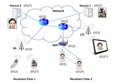
Figure 1: Fulcrum network codes allow sources and receivers to operate at higher field sizes to achieve high performance but maintaining compatibility with the $GF(2)$–only network. Receivers can choose to trade–off delay with decoding effort by choosing to decode with $GF(2)$ or in higher fields.

After more than a decade of research and in spite of NC’s theoretical gains in throughput, delay, and energy performance, its wide spread assimilation remains elusive. One, if not the most, critical weakness of the technology is the inherent complexity that it introduces into network devices. This complexity is driven by two factors. First, devices must perform additional processing, which may limit the energy efficiency gains or even become a bottleneck in the system’s overall throughput if processing is slower than the incoming/outgoing data rates. This additional effort can be particularly onerous if we consider that the conventional wisdom dictates that large field sizes are needed to provide high reliability, throughput, and delay performance. In addition to the computational burden, the use of high field sizes comes at the cost of a higher signaling overhead to communicate the coefficients used for coding the data packets. Other alternatives, e.g., sending a seed for a pseudo-random number generator, are relevant end-to-end but do not allow for a simple recoding mechanism. Interestingly, [14] showed that using moderate field sizes, specially $GF(2)$ , is key to achieving a reasonable trade-off among computational complexity, throughput performance, and total overhead specially when recoding data packets. This is particularly encouraging since $GF(2)$ performing encoding/decoding could be as fast as $160$ Mbps and $9600$ Mbps in a 2009 mobile phone and laptop [15], respectively, while in 2013 the speeds increased by five-fold in high-end phones [16]. Even limited sensors, e.g., TelosB motes, can generate packets in $GF(2)$ at up to $500$ kbps [17].

Second, devices must support different configurations for each application or data flow, e.g., different field sizes, to achieve a target performance. Supporting disparate configurations translates into high costs in hardware, firmware, or software. In computationally constrained devices, e.g., sensors, the support for encoding, recoding, or decoding in higher fields is prohibitive due to the processing effort required. On the other end of the spectrum, computationally powerful devices may also be unable to support multiple configurations. For example, high-load, high-speed Internet routers would require deep packet inspection to determine the coding configuration, followed by a different treatment of each incoming packet. This translates into additional expensive hardware to provide high-processing speeds. Additionally, intermediate nodes in the network are heterogeneous in nature, which limits the system’s viable configurations.

A separate, yet related practical issue is the fact that receivers interested in the same data flow may have wildly different computational, display, and battery capabilities as well as different network conditions. This end-device heterogeneity may restrict service quality at high-end devices when support is required for low-end devices, may deny service to low end devices for the benefit of high end ones, or require the system to invest additional resources supporting parallel data flows, each with characteristics matching different sets of users.

A clear option to solve the compatibility and complexity challenges is to limit sources, intermediate nodes, and receivers to use only $GF(2)$. However, using only $GF(2)$ may deprive higher-end devices of achieving higher reliability and throughput performance. Is it possible to provide a single, easily implementable, and compatible network infrastructure that supports flows with different end-to-end requirements?

This paper shows that the solution, called Fulcrum network codes, is simple, tunable, and surprisingly powerful. This is a framework that hinges on using only $GF(2)$ operations in the network (Fig. 1), to achieve reduced overhead, computational cost, and compatibility to heterogeneous devices and data flows in the network, while providing the opportunity of employing higher fields end-to-end via a tunable and straightforward precoding mechanism for higher performance. Fig. 1 shows an example, where two sources operate using different fields $GF(2^{h})$ and $GF(2^{b})$ for source 1 and 2, respectively. The intermediate nodes in the network use only $GF(2)$ operations. With Fulcrum network codes, the left-most receiver of flow 1 in Fig. 1 can choose to decode using $GF(2)$ only as it has limited computation capabilities. Since the left-most receiver of flow 2 has a better channel than other devices and the router may have to broadcast for a longer time due to the other receivers, the left-most receiver can choose to save energy on computation by accumulating additional packets and decoding using $GF(2)$. Furthermore, this receiver can also recode packets and send them to a neighbor interested in the same content, thus increasing the coverage of the system and reducing the number of transmissions needed to deliver it.

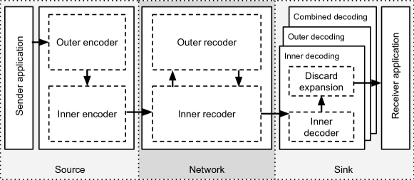
Figure 2: Description of system showing the inner and outer code structures. The outer code is typically established end-to-end. Although some applications could use outer recoders at intermediate nodes for higher efficiency in the network, in most scenarios the inner recoder is enough for supporting the desired functionalities. The sinks can choose from three main types of decoders: the inner, the outer, and the combined decoders. The outer can be exploited with any configuration of outer/inner codes, while the inner and combined decoders require a specific structure of the outer code, e.g., systematic.

II Description of the Scheme

The key goals of Fulcrum network codes are the following:

1. Reduce the overall overhead of network coding by (a) reducing the overhead due to coding coefficients per packet, and (b) reducing the overhead due to transmission of linearly dependent packets.

2. Provide simple operations at the routers/devices in the network. The key is to make recoding at these devices as simple as possible, without compromising network coding capabilities.

3. Enable a simple and adaptive trade-off between performance and complexity.

4. Support compatibility with any end-to-end linear erasure code in $GF(2^{h})$.

5. Control and choose desired performance and effort in end devices, while intermediate nodes provide a simple, compatible layer for a variety of applications.

II-A Idea

The key technical idea of Fulcrum is the use of a dimension expansion step, which consists of taking a batch of $n$ packets, typically called a generation, from the original file or stream and expand into $n+r$ coded packets, where $r$ coded packets contain redundant information and are called expansion packets. After the expansion, each resulting coded packet is treated as a new packet that will be coded in $GF(2)$ and sent through the network. The mapping for this conversion is known at the senders and at the receivers a priori.

Since additions in any field of the type $GF(2^{k})$ is simply a bit-wise XOR, the underlying linear mapping in higher fields can be reverted at the receivers. The reason to do the expansion is related to the performance of $GF(2)$, which can introduce non-negligible overhead in some settings [7, 18]. More specifically, coded packets have a higher probability of being linearly dependent when more data is available at the receiver. Increasing dimensions addresses this problem by mapping back to the high field representation after receiving $n$ linearly independent coded packets and decoding before the probability of receiving independent combinations in $GF(2)$ becomes prohibitive. The number of additional dimensions, $r$, controls the decoding probability performance. The larger the $r$, the better the performance achieved by the receivers while still using $GF(2)$ in the network.

Our approach naturally divides the problem in the design of inner and outer codes, using the nomenclature of concatenated codes [19]. Concatenating codes is a common strategy in coding theory, but typically used solely for increasing throughput performance point-to-point [19] or end-to-end, e.g., Raptor codes [20]. Some recent work on NC has considered the idea of using concatenation to (i) create overlapping generations to make the system more robust to time-dependent losses, but using the same field size in the inner and outer code [21]; (ii) decompose the network in smaller sub-networks in order to simplify cooperative relaying [22]; (iii) connecting NC and error correcting channel coding, e.g., [23]; or (iv) subspace codes for noncoherent network coding [24]. Fulcrum is fundamentally disruptive in two important ways. First, we allow the outer code to be agreed upon by the sources and receivers (dimension expansion), while the inner code is created in the network by recoding packets. Thus, we provide a flexible code structure with controllable throughput performance. Second, it provides a conversion from higher field arithmetic to $GF(2)$ to reduce complexity.

Dividing into two separate codes has an added advantage, not envisioned in previous approaches. This advantage comes from the fact that the senders can control the outer code structure to accommodate heterogeneous receivers. The simplest way to achieve this is by using a systematic structure in the outer code. This provides the receivers with the alternative to decode in $GF(2)$ after receiving $n+r$ coded packets instead of mapping back to higher fields after receiving $n$ coded packets. This translates into less decoding complexity, as $GF(2)$ requires simple operations, but incurring higher delay. The latter comes from the fact that $r$ additional packets must be received.

If the precoding uses a systematic structure, the system can support three main types of receivers (See Fig. 2). First, a computationally powerful receiver that decodes in $GF(2^{h})$ by mapping back from the $GF(2)$ combinations received. We call this the outer decoder. This procedure is simple because the addition for any extension field $GF(2^{l})$ is the same as that to $GF(2)$, namely, a bit-by-bit XOR. We show that accumulating $n$ linearly independent $GF(2)$ coded packets is enough to decode in the higher field. A receiver that decodes in $GF(2)$ reduces its decoding complexity but needs to gather $n+r$ independent linear combinations. Finally, we show that a hybrid decoder is possible, which can maintain the high decoding probability when receiving $n$ coded packets as in the high-field decoder, while having similar decoding complexity to that of the inner decoder. We call this hybrid decoder the combined decoder.

Our work is inspired in part by [25], which attempted to maintain overhead limited to a single symbol per packet. Thomos et al. made a very careful design in their packet coding at the source, but the end result is seemingly disappointing because only a small number of packets could be transmitted maintaining the overhead at one symbol. However, we argue that their careful code construction is not really needed. In fact, the reason behind their results is dominated by the network operations and their strict overhead limitation and not the source code structure, as we will show in this paper. Through our simple design framework, we break free from the constraint of a single symbol overhead and discover the potential to (i) reduce the overhead per packet in the network to roughly that of an end to end $GF(2)$ RLNC system (which is equivalent to the overhead reported in [25]), (ii) trade-off performance in the presence of heterogeneous receivers exploiting a family of precoders and simple designs, and (iii) exploit any generation size without introducing a synthetic constraint due to the field size at the precoder. The work in [25] is a special subcase of our general framework.

II-B Design

The overall framework is described in Fig. 2, showing the actions of the source, the network, and the destinations. In the following, we describe these actions in more detail.

II-B1 Operations at the Source

using the $n$ original packets, $P_{1},P_{2},...,P_{n}$, the source generates $n+r$ coded packets, $C_{1},C_{2},...,C_{n+r}$ using $GF(2^{h})$ operations (See Fig. 2-Source). The additional $r$ coded packets are called expansion packets. After generating these coded packets, the source re-labels these as mapped packets to be sent through the network and assigns them binary coefficients in preparation for the $GF(2)$ operations to be carried in the network. Finally, the source can code these new, re-labeled packets using $GF(2)$. The $i$-th coded packet has the form $\sum_{j=1}^{n+r}\lambda_{i,j}C_{j}$. The coding over $GF(2)$ is performed in accordance with the network’s supported inner code. For example, if the network supports $GF(2)$ RLNC, the source generates RLNC coded packets. However, other inner codes, e.g., perpetual [26], tunable sparse network coding [27, 28], are also supported.

Our main design constraint is that the receiver should (i) decode with the $n+r$ coded packets, and more importantly (ii) that it can decode with high probability after the reception of $n$ coded packets. Given that the structure of the initial mapping is controlled by the source, we could use Reed-Solomon (RS) codes, which are known end-to-end, or send the seed that was used to generate the mapping with each packet for a random code. In order to cater to the capabilities of heterogeneous receivers, we suggest the use of a systematic expansion/mapping, which already guarantees condition (i) but also provides interesting advantages for computationally constrained receivers. This is explained in more detail in the operations of the receivers.

II-B2 Operations at Intermediate Nodes

The operations at the intermediate nodes are quite simple (Fig. 2-Network). Essentially, they will receive coded packets in $GF(2)$ of the form $\sum_{j=1}^{n+r}\lambda_{i,j}C_{j}$, store them in their buffers, and send recoded versions to the next hops, typically implementing an inner decoder as described in the following. The recoding mechanism is what defines the structure of the inner code of our system. Recoding can be done as a standard $GF(2)$ RLNC system would do, i.e., each packet in the buffer has a probability of $1/2$ to be XORed with the others to generate the recoded packet. However, the network can also support other recoding mechanisms, such as recoding for tunable sparse network coding [27, 28] and for Perpetual network codes [26], or even no recoding. We shall discuss the effect of several of these inner codes as part of Section IV.

In some scenarios, it may be possible to allow intermediate nodes to know and exploit the outer code in the network (Fig. 2-Network). The main goal of these recoders is to maintain recoding with $GF(2)$ operations only. However, when the intermediate node gathers $n$ linearly independent coded packets in the inner code, it can choose to map back to the higher field in order to decode the data and improve the quality of the recoded packets. The rationale is that, at that point, it can recreate the original code structure and generate the additional dimensions $r$ that are missing in the inner code, thus speeding up the transmission process. Although not required for the operation of the system, this mechanism can be quite useful if the network’s intermediate nodes are allowed to trade-off throughput performance with complexity.

II-B3 Operations at the Receivers

We consider three main types of receivers assuming that we enforce a systematic outer code. Of course, intermediate operations or other precoding approaches can be used enabling different end-to-end capabilities and requirements.

Receivers using an Outer Decoder will map back to the original linear combination in $GF(2^{h})$ (See Fig. 3-left). This means that only decoding of an $n\times n$ matrix in the original field is required. The benefit is that the receiver decodes after receiving $n$ independent coded packets in $GF(2)$ with high probability. The key condition is that the receivers need to know the mapping in $GF(2^{h})$ to map back using the options described for the source. These receivers use more complex operations for decoding packets, but are awarded with less delay than $GF(2)$ to recover the necessary linear combinations to decode. We will show that increasing $r$ yields an exponential decrease of the overhead due to non-innovative packets, i.e., coded packets that do not convey a new independent linear combination to the receiver.

On the other hand, receivers using an Inner Decoder opt to decode using $GF(2)$ operations for the $n+r$ relabelled packets (See Fig. 3-middle). This is known to be a faster, less expensive decoding mechanism although there is some additional cost of decoding a $(n+r)\times(n+r)$ matrix. If the original mapping uses a systematic structure, decoding in this form already provides the original packets without additional decoding in $GF(2^{h})$. The penalty for this reduced computational effort is the additional delay incurred by having to wait for $n+r$ independent linear combinations in $GF(2)$. Thus, there is no benefit over standard $GF(2)$ but we provide compatibility with the other nodes.

Finally, receivers using a Combined Decoder implement a hybrid between inner and outer decoders with the aim of approaching the decoding speed as inner decoders while retaining the same decoding probability as outer decoders (See Fig. 3-right). This is achieved by decoding the first $n$ coded packets using $GF(2)$ only. If decoding is unsuccessful in $GF(2)$, all coded packets are mapped to $GF(2^{h})$ over which the remaining decoding is performed. Hence, if $r<<n$ the decoding cost of the last $r$ is negligible compared to that of the initial $n$ packets and decoding speed will approach that of an inner decoder. We show this in Section V.

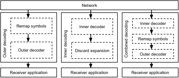
Figure 3: Overview of components of the three types of Fulcrum decoders. Each decoder operates on the same data stream coming from the network. This makes it possible to support heterogeneous receivers using some mix of the three decoding types.

II-C Benefits

II-C1 Simple is Green, Compatible, and Deployable

The bit-wise XOR operations of $GF(2)$ in the network are easy and cost-effective to implement in software/hardware and also energy efficient because they require little processing. Their simplicity makes them compatible with almost any device and can be processed at high-speed. Having a simple approach where all packets in the network are processed using $GF(2)$, reduces the additional logic and processing in intermediate nodes.

II-C2 Supports Heterogeneous Receivers

The use of an inner decoder is not only an option for resource-limited devices. It can be a tool to reduce the decoding effort at receivers, in particular if $r$ is small. This is possible if the outer code has a systematic structure, which allows for a direct recovery of the original packets once decoding happens in $GF(2)$, or other structure for the outer code, that allows for a fast decoding, e.g., sparse outer code, Jacket matrix structure [29]. For example, consider the case of a single hop broadcast network with heterogeneous channels. A device that has the best channel of the receivers could choose to wait for additional transmissions from the source, given that those transmissions will happen in any case and the receiver might still invest energy to receive them (e.g., to wait for the next generation). The additional receptions can be used to decode using $GF(2)$ instead of doing the mapping to decode in $GF(2^{h})$ in this way reducing the energy invested in decoding. On the other hand, a receiver with a bad channel will attempt to use $GF(2^{h})$ to decode in order to reduce its overall reception time.

II-C3 Adaptable Performance

Fulcrum can be configured to cover a wide range of decoding complexity vs. throughput performance tradeoffs if we consider the use of sparse outer codes. Let us illustrate this potential with a simple outer code with a density $d$, i.e., the fraction of non-zero coefficients. Let us consider some extreme cases. First, the case of no extension $r=0$ and $d\approx\frac{n}{2}$, which corresponds to a binary RLNC code. Second, the case of no extension $r=0$ and $d<<\frac{n}{2}$, which corresponds to a sparse binary RLNC code. Also, $r>>n$, $d=1$, can achieve similar performance to RLNC with a high field size. By adjusting $r$ and $d$, Fulcrum can be tuned to the desired complexity - throughput tradeoff. Importantly, these parameters can also be changed on-the-fly, allowing for adoption to time varying conditions. Of course, the choice of outer code need not be only changed with the $d$ parameter. In fact, an LT code, Perpetual code, or Tunable Sparse Network Code could also be used for providing additional trade-offs.

II-C4 Practical Recoding

Recoding can be performed exclusively over the inner code, while encoding and decoding is performed over the outer code. As the inner code is in $GF(2)$, its coding vector can easily be represented compactly, which solves the challenge associated with enabling recoding when a high field size is used [14].

II-C5 Spreading Complexity Across the Network

Both intermediate nodes and receivers can choose the computational complexity they are capable of dealing with. This enables the complexity to be spread across nodes in the network. Although we currently focus on $n$ independent decision between receivers, future work could consider a network that controls what devices will invest more computational effort for specific flows.

II-C6 Security

If security is the goal, our scheme provides a simple way to implement some of the ideas in SPOC [30]. With Fulcrum, the mapping of the outer decoder constitutes the secret key (or part of it) that the source and destinations share and that, in contrast to [30], need not be sent over the network along with the coded packets. Using Fulcrum, we will not incur the large overhead of SPOC, which sends two coding coefficients per original packet (one encrypted, one without encryption). In fact, the end points (source and receivers) can choose very large field sizes in the outer code while maintaining $1+r/n$ bits per packet in the generation as overhead. Fulcrum can also provide security without the need to run Gaussian elimination twice at the time of decoding [31]. As a consequence Fulcrum does not need to trade–off field size and generation size (and thus security) for overhead in the network and complexity.

II-C7 New Designs while Supporting Backwards Compatibility

Exploiting one code in the network and one underlying code end-to-end provides senders and receivers with the flexibility to control their service requirements while making the network agnostic to each flows’ characteristics. This has another benefit: new designs and services can be incorporated with minimal or no effort from the network operator and maintaining backward compatibility.

III Analysis of Receiver Performance with RLNC as Inner Code

Let us understand the delay performance in receivers using the outer and combined decoders. Receivers using an inner decoder correspond to a $GF(2)$ receiver that needs to get $n+r$ independent linear combinations before decoding [7, 15, 18]. The key question is to determine whether receiving $n$ independent coded packets in $GF(2)$ means that the re-mapped version in $GF(2^{h})$ is full rank, i.e., original data can be decoded. Section III-A shows that this is possible for a RS outer code under some minor conditions.

III-A Decoding Performance with a Reed-Solomon Outer Code

We have $B$, an $m\times n+r$-matrix over ${\mathbb{F}}_{2}$, and $G$, an $(n+r)\times n$-matrix over ${\mathbb{F}}_{2^{s}}={\mathbb{F}}_{q}$. We have that $G$ is the generator matrix of a RS code with length $n+r\leq q-1=2^{s}-1$. The value of $m$ is related to the length of the incoming messages, e.g., if it is a single ${\mathbb{F}}_{2^{s}}$ symbol, then $m=s$ bits. We remark that vectors are column vectors and that we multiply on the right.

A RS code $C$, with dimension $n$, can be defined as the vector space generated by the evaluation of the monomials $1,X,\ldots,X^{n-1}$ at the points ${\mathbb{F}}_{q}\setminus\{0\}$. Namely, let $\alpha$ be a primitive element of ${\mathbb{F}}_{q}$ and let ${\text{ev}}:{\mathbb{F}}_{q}[X]\to{\mathbb{F}}_{q}^{n+r}$, given by ${\text{ev}}(f)=(f(\alpha^{0}),f(\alpha^{1}),\ldots,f(\alpha^{q-2})$. One has that $C=\langle\{{\text{ev}}(X^{i}):i=0,\ldots,n-1\}\rangle$. A generator matrix is given by considering as columns the evaluation of a monomial at ${\mathbb{F}}_{q}\setminus\{0\}$. The dual code of a RS code is given by Lemma 1.

Lemma 1.

(Lemma 5.3.1 [32]) Let $C$ be a Reed-Solomon code with dimension $n$, then the dual code of $C$ is given by $C^{\perp}=\langle\{{\text{ev}}(X^{1}),\ldots,{\text{ev}}(X^{q-1-n})\}\rangle$

We consider the $m\times n$-matrix $BG$ and denote the associated linear function by $\varphi$. We assume that $B$ and $G$ have full rank and we wonder whether $\dim(\varphi(V))<\dim V$ for a vector subspace $V\subseteq{\mathbb{F}}_{q}^{n}$. Since $\varphi$ is a linear function, one has that the dimension of the image plus the dimension of the kernel is equal to the dimension of the original space. Therefore, we wonder whether, $\dim(\ker(\varphi))>0$.

In order to prove the main result, we shall introduce the cyclotomic coset containing $a$ in ${\mathbb{F}}_{q}={\mathbb{F}}_{2^{s}}$, $I_{a}=\{a,2a{\text{~{}mod~{}}}q-1,2^{2}a{\text{~{}mod~{}}}q-1,\ldots,2^{s-1}a{\text{~{}mod~{}}}q-1\}$. For instance, for $q=2^{4}$, the different cyclotomic cosets are $I_{0}=\{0\},I_{1}=\{1,2,4,8\},I_{3}=\{3,6,12,9\},I_{5}=\{5,10\},I_{7}=\{7,14,13,11\}.$ One has that $I_{1}=I_{2}=I_{4}=I_{8}$, but usually one denotes the coset by the smallest number. We can now characterize when $\dim(\ker(\varphi))=0$.

Theorem 2.

Let $C\subseteq{\mathbb{F}}_{2^{s}}={\mathbb{F}}_{q}$ be a Reed-Solomon code with dimension $n$ and the linear map $\varphi$ defined above. One has that $\dim(\ker(\varphi))=0$ if and only if $n\geq 2^{s-1}$.

Proof.

One has that $\varphi$ is the composition of two linear maps, the ones associated to $G$ and $B$. We have that $G$ is a generator matrix and therefore, it is injective. Hence, $BGx=0$ if and only if $c=Gx\in\ker(B)$. That is, $\dim(\ker(\varphi))>0$ if the rows of $B$ are orthogonal to $c$, which is a word of $C$. Therefore, the rows of $B$ are words in the dual code of $C$.

By Lemma 1, the dual code of $C$ is given by $C^{\perp}=\langle\{{\text{ev}}(X^{1}),\ldots,{\text{ev}}(X^{q-1-n})\}\rangle$. We have that $C^{\perp}\subseteq{\mathbb{F}}_{q}^{n+r}$ but the rows of $B$ are over ${\mathbb{F}}_{2}$. Hence we should consider the subfield subcode of $C^{\perp}$, that is

$${\text{SubfieldSubcode}}_{2}(C^{\perp})=\{c\in{\mathbb{F}}_{2}^{n+r}:c\in C^{\perp}\}.$$

The columns of the generator matrix of ${\text{SubfieldSubcode}}_{2}(C^{\perp})$ are the rows of $B$ which reduce the dimension of the image. By [33] and [34, Theorem III.8], one has that

$$\dim({\text{SubfieldSubcode}}_{2}(C^{\perp}))=\#\{I_{j}:I_{j}\subseteq\{1,\ldots,q-1-n\}\}.$$

That is, we shall only consider exponents that are in a cyclotomic coset that is contained in $\{1,\ldots,q-1-n\}$. Clearly $I_{0}\not\subseteq\{1,\ldots,q-1-n\}$. Let $k\geq 2^{s-1}$, then one has that $q-1-n<2^{s-1}$ and therefore the cyclotomic coset $I_{1}=\{1,2,2^{2},\ldots,2^{s-1}\}$ is not contained in $\{1,\ldots,q-1-n\}$. Finally, let $j>2^{s-1}$, then $I_{j}\neq I_{0},I_{1}$, and we have that $I_{j}\not\subseteq\{1,\ldots,q-1-n\}$ since $j\in I_{j}$ and $q-1-n<2^{s-1}$. Therefore ${\text{SubfieldSubcode}}_{2}(C^{\perp})=\{0\}$ and $\dim(\ker(\varphi))=0$.

Let us consider now $n<2^{s-1}$, then $I_{1}=\{1,2,2^{2},\ldots,2^{s-1}\}$ is contained in $\{1,\ldots,q-1-n\}$ and $\dim({\text{SubfieldSubcode}}_{2}(C^{\perp}))\geq s$. Thus $\dim(\ker(\varphi))>0$. ∎

Explicit generators of ${\text{SubfieldSubcode}}_{2}(C^{\perp})$ to identify cases of linear dependence for $n<2^{s-1}$ can be obtained by using results in [33], [34, Theorem III.8] as follows.

Theorem 3.

Let $C$ be a Reed-Solomon code with dimension $n$, the dimension of ${\text{SubfieldSubcode}}_{2}(C^{\perp})$ is $\sum_{I_{a}\subseteq\{1,\ldots q-1-n\}}\#I_{a},$ and a basis is given by $\{{\text{ev}}(f_{I_{a},\beta^{j}}):j\in\{0,\ldots,\#I_{a}-1\}\},$ where $\beta=\alpha^{(2^{s}-1)/(2^{\#I_{a}}-1)}$, i.e. a primitive element of ${\mathbb{F}}_{2^{\#I_{a}}}\subseteq{\mathbb{F}}_{2^{s}}$, and $f_{I_{a},\beta}=\beta X^{a}+\beta^{2}X^{2a}+\cdots+\beta^{2^{\#I_{a}-1}}X^{2^{\#I_{a}-1}a}$.

As an example, let $C_{8}$ be the Reed-Solomon code with dimension $n=2^{3}$ in ${\mathbb{F}}^{15}_{2^{4}}$. We have that $C_{8}=\langle\{{\text{ev}}(X^{0}),\ldots,{\text{ev}}(X^{7})\}\rangle$, $C_{8}^{\bot}=\langle\{{\text{ev}}(X^{1}),\ldots,{\text{ev}}(X^{7})\}\rangle$ and ${\text{SubfieldSubcode}}_{2}(C_{8}^{\perp})=\{0\}$ because $I_{a}\not\subseteq\{1,\ldots,7\}$ for any $a$ and $\dim(\ker(\varphi))=0$. Consider another example with a Reed-Solomon code $C_{7}$ with dimension $n=7$ in ${\mathbb{F}}^{15}_{2^{4}}$. We have that $C_{7}=\langle\{{\text{ev}}(X^{0}),\ldots,{\text{ev}}(X^{6})\}\rangle$, $C_{7}^{\bot}=\langle\{{\text{ev}}(X^{1}),\ldots,{\text{ev}}(X^{8})\}\rangle$ and $\dim({\text{SubfieldSubcode}}_{2}(C_{7}^{\perp}))=4$ because $I_{1}=\{1,2,4,8\}\subseteq\{1,\ldots,8\}$. A basis for ${\text{SubfieldSubcode}}_{2}(C_{7}^{\perp})$ is given by $\{{\text{ev}}(f_{I_{1},1}),{\text{ev}}(f_{I_{1},\alpha}),{\text{ev}}(f_{I_{1},\alpha^{2}}),{\text{ev}}(f_{I_{1},\alpha^{3}})\}$, that is

$$\{{\text{ev}}(X+X^{2}+X^{4}+X^{8}),{\text{ev}}(\alpha X+\alpha^{2}X^{2}+\alpha^{4}X^{4}+\alpha^{8}X^{8}),$$

$${\text{ev}}(\alpha^{2}X+\alpha^{4}X^{2}+\alpha^{8}X^{4}+\alpha X^{8}),{\text{ev}}(\alpha^{3}X+\alpha^{6}X^{2}+\alpha^{12}X^{4}+\alpha^{9}X^{8})\}.$$

Therefore, a generator matrix for ${\text{SubfieldSubcode}}_{2}(C_{7}^{\perp})$ is

$$\scalebox{0.8}{$\begin{bmatrix}000100110101111\\ 001001101011110\\ 010011010111100\\ 101110101111000\end{bmatrix}$}^{T}.$$

Future work shall consider exploiting such generators to improve the efficiency of the decoder in these corner cases. In order to consider $\beta$ as a primitive element of ${\mathbb{F}}_{2^{\#I_{a}}}$ in ${\mathbb{F}}_{2^{s}}$, one may consider to use Conway polynomials for defining finite fields [35].

III-B Delay Modelling and Performance

We focus on the analysis for a single receiver first to understand the potential. For the analysis, let us assume that a RS code over $GF(2^{s})$ and $n\geq 2^{s-1}$ is used for the outer code, so that receiving $n$ independent coded packets in $GF(2)$ guarantees that the re-mapped version in $GF(2^{h})$ can be decoded (using the result from Theorem 2). We reuse the models for RLNC coding from [18, 7]. Fig. 4 (a) shows the Markov chain representing the process of reception of independent linear combinations at the receiver given the reception of a new coded packet over $GF(2)$ using an RLNC inner code. Each stage represents the missing independent linear combinations in $GF(2)$ in order to decode using only $GF(2)$ operations. In this case, we assume that the receiver is attempting to decode in $GF(2)$ even when the source has made an expansion to $n+r$ dimensions. This corresponds to a receiver using an inner decoder. Fig. 4 (b) on the other hand shows the process for a successful outer (and combined) decoder. In this case, the underlying $GF(2)$ process needs only run until $n$ independent linear combinations in $GF(2)$ are received, which are mapped back into the $GF(2^{h})$ and decoded for the outer decoder. The combined decoder performs partial decoding in $GF(2)$ before attempting to use the high field, but this does not affect the following analysis, only decoding complexity. Thus, the last states starting in $r-1$ until $0$ are not visited, as state $r$ became an absorbing state. If a different precoding structure is used, there will be some probability of visiting the states beyond $r$. However, if we use a large enough field size, this effect will be negligible and the process described in Fig. 4 (b) will be a very good approximation of the expected performance. Using the intuition from Fig. 4 (b), the mean number of packets received from the network to decode using an outer (or combined) decoder considering $r$ additional dimensions is given by

$$E\left[N_{GF(2)}(r)\right]=\sum_{i=r+1}^{n+r}\frac{1}{1-2^{-i}}=n+\sum_{i=r+1}^{n+r}\frac{1}{2^{i}-1}.$$ (1)

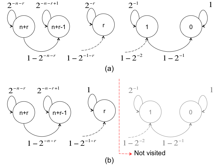
Figure 4: Markov Chain describing the reception process at a receiver in (a) a classical $GF(2)$ network, i.e., where both source and network use $GF(2)$ operations, and (b) exploiting our expansion idea, i.e., where the network treats expanded packets as $GF(2)$ packets while the source uses $GF(2^{h})$ operations for the expansion.

Lemma 4 shows that the overhead due to additional $GF(2)$ coded packet receptions when using an outer or combined decoder decreases exponentially with $r$.

Lemma 4.

Considering an outer or a combined decoder with an MDS inner code, we have $E\left[N_{GF(2)}(r)\right]=n+2^{-r}\times\theta(n)$, for some $\theta(n)\in[1-2^{-n},2-2^{-n+1}]$.

Proof.

The proof follows from finding an upper and lower bound on $E\left[N_{GF(2)}(r)\right]$ described in Eq. (1). To derive the upper bound, we use the fact that $2^{i-1}\leq 2^{i}-1$ for $i\geq 1$ to convert into the sum of a set of elements of the geometric series. Thus, $E\left[N_{GF(2)}(r)\right]\leq n+\sum_{i=r+1}^{n+r}2^{-i+1}=n+2^{-r+1}-2^{-n-r+1}.$The lower bound follows a similar argument, but using the fact that $2^{i}\geq 2^{i}-1$ for $i\geq 1$. Thus, $E\left[N_{GF(2)}(r)\right]\geq n+\sum_{i=r+1}^{n+r}2^{-i}=n+2^{-r}-2^{-n-r}.$∎

Another interesting result for receivers with outer and combined decoders is shown in Lemma 5, where we proof that the variance of $N_{GF(2)}(r)$ decreases exponentially with $r$.

Lemma 5.

Considering a receiver using an outer or combined decoder with an MDS inner code, then $var\left(N_{GF(2)}(r)\right)=O(2^{-r}).$

Proof.

The proof follows by bounding the variance of $N_{GF(2)}(r)$. Defining $P_{i}=1-2^{-n-r+i-1}$ and using independence in the Markov chain, it is straightforward to prove that $var\left(N_{GF(2)}(r)\right)=\sum_{i=1}^{n}\frac{1-P_{i}}{P_{i}^{2}}$. After some manipulations and using the fact that $2^{-r-1}\geq 2^{-n-r+i-1}$ for $i=1,...,n$ then,

$$var\left(N_{GF(2)}(r)\right)=\sum_{i=1}^{n}\frac{1}{\left(1-2^{-n-r+i-1}\right)^{2}}-E\left[N_{GF(2)}(r)\right]\leq\frac{E\left[N_{GF(2)}(r)\right]}{2^{r+1}-1}\leq\frac{n+2^{-r+1}}{2^{r+1}-1},$$ (2)

which concludes the proof. ∎

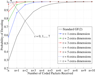
(a)

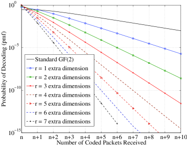
(b)

Figure 5: Successful decoding for an outer or combined decoder given $r$ redundant dimensions: (a) CDF and (b) PMF

Fig. 5a shows the cumulative distribution function (CDF) for a receiver with an outer or a combined decoder and with a network operating with $GF(2)$ and various values of $r$. Clearly, introducing additional dimensions improves the probability of decoding with fewer received coded packets from the network. In fact, even for a small value, e.g., $r=1$ or $r=2$, the improvement is quite noticeable. This is good from a practical perspective as these gains can be achieved without dramatically decreasing performance in the receivers using inner decoders. Table I provides key decoding probabilities (in percentages) when receiving $n$, $n+1$, $n+2$, and $n+3$ coded packets when the inner code is RLNC $GF(2)$. Better results could be obtained if using a systematic structure. The table shows that the probability of decoding after receiving exactly $n$ coded packets using an outer or combined decoder is quite high even for moderate $r$ values. It also shows that the performance with $r=7$ is similar to that provided by RaptorQ codes [36], while $r>7$ can provide higher decoding guarantees. The corresponding probability mass function (PMF) is presented in Figure 5b. This shows that the variance is reduced with the increase of $r$ and that even a $r>4$ reduces the probability of transmitting more than $n$ coded packets before decoding by at least an order of magnitude with respect to RLNC over $GF(2)$.

Code		Decoding after receiving (coded packets)
Fulcrum	$\mathbf{r}$	$\mathbf{n}$	$\mathbf{n+1}$	$\mathbf{n+2}$	$\mathbf{n+3}$
	4	93.87%	99.75%	99.99%	99.9997%
	7	99.22%	99.996%	99.99998 %	99.99999992%
	10	99.90%	99.9999%	99.99999996%	99.99999999998%
RaptorQ		99%	99.99%	99.9999%

TABLE I: Decoding after reception of a certain number of coded packets using the outer or combined decoders for various $r$ and assuming RLNC $GF(2)$ inner encoder and recoders.

III-C Extension to Broadcast with Heterogeneous Receivers

Let us consider the case of broadcast from one source to two receivers ($R_{1}$ and $R_{2}$) with independent channels and packet loss probability $e_{i}$ for receiver $R_{i}$. Our goal is to illustrate the effect of using different decoders at receivers with heterogeneous channel qualities as well as to compare the performance of Fulcrum to that of standard RLNC at different finite fields.

We exploit the Markov chain model presented in [7] to provide an accurate representation of the field size effect when broadcasting to two receivers. This model is also easily adapted to incorporate the use of the outer decoding capabilities of Fulcrum. The model in [7] relies on a state definition that incorporates three variables, the number of independent linear combinations at each receiver and the common linear combinations between the two. The key change in the model is similar to the change introduced in the Markov chain in Section III, that is, considering that the dimensions in the Markov chain in [7] have a higher number of possible values, namely, $n+r+1$ instead of $n+1$ per variable in the state. Then, if one (or both) receivers use the outer (or combined) decoder, the number of linear combinations gathered by that receiver will be increased to $n+r$ whenever the receiver would normally achieve $n$. Using these modifications, we generated the results for Figure 6a.

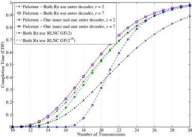
(a)

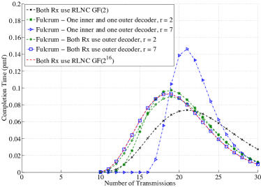
(b)

Figure 6: (a) CDF and (b) PMF of successful Decoding for Broadcast channel with two receivers showing the performance of standard RLNC for $GF(2)$ and $GF(2^{16})$, the performance of Fulcrum when one receiver exploits the outer code and the other only the inner code, and Fulcrum when both receivers exploit the outer code. Parameters $e_{1}=0.1$, $e_{2}=0.5$, $n=10$ packets.

Figure 6a shows the CDF for the number of transmissions to complete $n=10$ packets to two receivers. The performance of RLNC $GF(2^{16})$ shows the best performance of the best solution. Clearly, a Fulcrum approach where both receivers exploit the outer decoder and use $r=7$ redundant packets performs essentially the same as RLNC with $GF(2^{16})$. Note that Fulcrum with $r=2$ and two receivers with outer decoder provides close to the same performance as RLNC with $GF(2^{16})$ but with less complexity. Additionally, $r=2$ provides a much better trade–off for the two receivers using different decoders. Also, interesting is that even when one of the receivers attempts to decode using the inner decoder, i.e., using only $GF(2)$ operations, the worst case behavior is maintained. This worst case behavior is superior to using only RLNC with $GF(2)$. Figure 6b provides the PMF for a similar scenario, demonstrating that the variance using Fulcrum is reduced, particularly when increasing $r$. In fact, we observe that for the case of two receivers using Fulcrum’s outer (or combined) decoder achieve essentially the same PMF as RLNC with $GF(2^{16})$.

III-D Overhead

Let us define the overhead for a generation with size $n$ as the number of additional bits transmitted to successfully deliver a generation of packets including coding coefficients and linearly dependent packets. This means that it incorporates both the additional header information and the overhead caused by retransmissions due to linear dependency. For our analysis, we consider receivers with outer and combined decoders and that we use the standard coding vector representation, i.e., a coefficient per packet is sent attached to the coded packet.

The mean overhead of using $GF(2^{h})$ is proportional to $hn^{2}$ bits for large enough $h$ considering that there are channel losses that affect the total number of packets transmitted. The mean overhead of our scheme is proportional to $E\left[N_{GF(2)}\right](n+r)\leq n^{2}+nr+(n+r)\Big{(}2^{-r}-2^{-n-r}\Big{)}$ if we use a standard coding vector representation. Since $r<<n$ for these cases, the overhead will be dominated by $n^{2}+n2^{-r}$, which is to say almost a factor of $h$ smaller than using $GF(2^{h})$. However, this can be further reduced if we use a sparse $GF(2)$ inner code.

IV Effect of Sparse Inner Codes

Beyond benefiting from sparse inner codes for reducing overhead, Fulcrum can provide fundamental benefits to sparse coding strategies as well. We consider the general case of static sparse structures, i.e., sparse inner codes that do not change in time. Results can be extended to time-variant schemes such as tunable sparse network coding [27].

For the general case of sparse matrices, we use the following bound.

Theorem 6.

(Theorem 1 of [37] ) The probability $p(i,n)$ of a received coded packet with density $\rho(i,n)\leq 1/2$ to be innovative when the receiver already has $i$ out of $n$ degrees of freedom is $p(i,n)\geq 1-(1-\rho(i,n))^{n-i}.$

If the number of non-zero coefficients is given by $k$, then the use of Fulcrum provides a $\rho=k/(n+r)$. Lemma 7 provides an upper bound for the general case of sparse inner codes.

Lemma 7.

Considering the problem of a sparse inner code with an MDS outer code, we have $E[S(n,r)]\leq n+n\left(\exp\left(\frac{k(r+1)}{n+r}\right)-1\right).$

Proof.

$$E[S(n,r)] \overset{(1)}{\leq}\sum_{i=0}^{n-1}\frac{1}{1-(1-\rho)^{n+r-i}}=\sum_{i=r+1}^{n+r}\frac{1}{1-\left(1-k/(n+r)\right)^{i}}$$ (3)

$$\overset{(2)}{\leq}\sum_{i=r+1}^{n+r}\frac{1}{1-\exp\left(-\frac{ik}{n+r}\right)}$$ (4)

where step $(1)$ uses the bound in Theorem 6, $(2)$ uses the fact that $\left(1-k/(n+r)\right)^{i}\leq\exp\left(-\frac{ik}{n+r}\right)$. Let us consider $q=\exp\left(\frac{k}{n+r}\right)$, then

$$E[S(n,r)] \leq\sum_{i=r+1}^{n+r}\frac{1}{1-q^{-i}}\overset{(3)}{\leq}n\frac{q^{r+1}}{q^{r+1}-1}=n\frac{\exp\left(\frac{k(r+1)}{n+r}\right)}{\exp\left(\frac{k(r+1)}{n+r}\right)-1}$$ (5)

where $(3)$ uses the fact that $q^{-i}\leq q^{-r-1},q>1,i\geq r+1$, which concludes the proof. ∎

A first conclusion, is that $\lim_{r\rightarrow\infty}E[S(n,r)]\leq n\frac{e^{k}}{e^{k}-1}=n\left(1+\frac{1}{e^{k}-1}\right).$This means that adding additional redundancy in the outer code leads to a bounded performance in terms of overhead. If $k=3$ or $k=4$ for a large outer code redundancy, the mean number of coded packets to be received in order to decode is below $1.05n$ and below $1.019n$, respectively. That is, less than $5$% and $2$% overhead. If we consider LT codes using an ideal soliton distribution, the mean number of non-zeros is given by $k\approx\ln(n+r)$ [38], and $r=\alpha n$ and $\alpha>0$, then $E[S(n,r)]\leq n+O\left(\frac{n^{1/(\alpha+1)}}{(1+\alpha)^{\alpha/(\alpha+1)}}\right)$. As an example, if $\alpha=1$, then $E[S(n,r)]\leq n\left(1+\frac{1}{\sqrt{2n}-1}\right)$ while $\alpha=2$ produces $E[S(n,r)]\leq n\left(1+\frac{1}{(3n)^{2/3}-1}\right)$. If $\alpha\rightarrow\infty$, the overhead vanishes.

For the special case of fixed $\rho$ irrespective of the number of coding symbols for generated in the outer code, i.e., $\rho(i,n)=\rho$, then

$$E[S(n,r)] \overset{(1)}{\leq}\sum_{i=r+1}^{n+r}\frac{1}{1-\left(1/(1-\rho)\right)^{-i}}\overset{(2)}{=}\sum_{i=r+1}^{n+r}\frac{1}{-B^{-i}}=\sum_{i=r+1}^{n+r}\frac{B^{i}}{B^{i}-1}$$ (6)

$$\overset{(3)}{\leq}n+\sum_{i=r+1}^{n+r}\frac{1}{B^{i-1}(B-1)}=n+\frac{B}{B-1}\sum_{i=r+1}^{n+r}B^{-i}$$ (7)

$$=n+\frac{B^{n+1}-B}{\left(B-1\right)^{2}B^{n+r}}=n+\frac{(1-\rho)^{r+1}}{\rho^{2}}-\frac{(1-\rho)^{n+r+1}}{\rho^{2}},$$ (8)

where step $(1)$ uses the bound in Theorem 6, $(2)$ considers making $B=\frac{1}{1-\rho}$, and $(3)$ uses $B^{i}\geq B^{i}-B^{i-1}$ for $B\geq 1$. For $\rho$ fixed, then $r\rightarrow\infty$ then $E[S(n,r)]$ tends to $n$.

V Implementation

In this section, we describe the implementation of different Fulcrum encoder and decoder variants. The descriptions presented here are based on our actual implementation of the algorithms in the Kodo network coding library [39]. For our initial implementation, we utilized two RLNC codes with the outer code operating in $GF(2^{8})$ or $GF(2^{16})$ and the inner code in $GF(2)$.

V-A Implementation of the Encoder

One advantage of Fulcrum is that the encoding is quite simple. Essentially, the two encoders can be implemented independently, where the outer encoder uses the $n$ original source symbols to produce $n+r$ input symbols for the inner encoder. In general, the inner encoder can be oblivious to the fact that the input symbols might contain already encoded data.

For the initial implementation we required all source symbols to be available before any encoding could take place. This is however not necessary in cases where both encoders support systematic encoding. In such cases, it would be possible to push the initial $n$ symbols directly through both encoders without doing any coding operations or adding additional delay. An illustration of this is shown in Fig. 7a, where a set of $n=8$ original symbols are sent with the outer encoder configured to build an expansion of $r=2$.

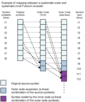
(a)

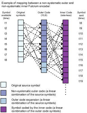
(b)

Figure 7: Example of (a) a systematic outer encoder and a systematic inner encoder with $n=8$ and $r=2$, and (b) a non-systematic outer encoder and a non-systematic inner encoder with $n=8$ and $r=2$

As both encoders in Fig. 7a are systematic, no coding takes place until step $9$ and $10$, where the outer encoder produces the first encoded symbols. At this point, the inner encoder is still in the systematic phase and therefore passes the two symbols directly through to the network. In step $11$, the inner encoder also exits the systematic phase and starts to produce encoded symbols. At this stage, the inner encoder is fully initialized and no additional symbols are needed from the outer encoder, all following encoding operations therefore take place in the inner encoder.

As shown in this simple example, using a systematic structure in both encoders can be very beneficial for low delay applications because packets can be sent as they arrive at the encoder. Systematic encoding is not always required for attaining this low delay. For example, if the inner encoder is a standard RLNC encoder only generating non-zero coefficients for the available symbols, i.e., using an on-the-fly encoding mechanism.

In the case of a non-systematic inner code, this low delay performance is typically not possible. However, there are several applications where non-systematic encoding may be more beneficial, e.g., for security, multiple-source and/or multiple-hop networks. For data confidentiality, using a systematic outer code becomes a weakness in the system. In this case, a dense, high field outer code is key to providing the required confidentiality.

As an example, Fig. 7b shows the use of a non-systematic outer encoder. Assuming the outer mapping is kept secret, only nodes with knowledge of the secret would be able to decode the actual content. Whereas all other nodes would still be able to operate on the inner code. For multi-hop networks or multi-source networks, a systematic inner code may not be particularly useful for the receiver as the systematic structure will not be preserved as the packet traverses the network and is recoded. Fig.  7b shows that it is also possible to use a non-systematic encoding scheme at the inner encoder. This is typically implemented to minimize the risk of transmitting linear dependent information in networks which may contain multiple sources for the same data, e.g. in Peer-to-Peer systems, or if the state of the sinks is unknown.

V-B Implementation of the Decoder

We have developed decoders supporting all three types of receivers mentioned in Section II.

Outer decoder: immediately maps from the inner to the outer code essentially decoding in $GF(2^{h})$. This type of decoder is shown in Fig. 8. In order to perform this mapping, a small lookup table storing the coefficients was used. The size of the lookup table depends on whether the outer encoder is systematic or not. In the case of a systematic outer encoder a lookup table of size $r$ is sufficient, since the initial $n$ symbols are uncoded (i.e. using the unit vector). However, in case of a non-systematic outer encoder all $n+r$ outer encoding vectors needs to be stored. An alternative approach would be to use a pseudo-random number generator to generate the encoding vectors on the fly as needed. One advantage of the lookup table is that it may be precomputed and therefore would not consume any additional computational resources during encoding/decoding.

Inner decoder: decodes using only $GF(2)$ operations, requiring a systematic outer encoder (Fig. 9a). In this case, the decoder’s implementation is very similar to a standard RLNC $GF(2)$ decoder configured to received $n+r$ symbols. The only difference being that only $n$ of the decoded symbols will contain the original encoded data. If sparse inner codes are used, other decoding algorithms could be used, e.g., belief propagation [20].

Combined decoder: attempts to decode as much as possible using the inner decoder before switching to the typically more computationally costly outer decoder. Note that this type of decoding only is beneficial if the outer encoder is systematic or, potentially, very sparse. Otherwise, the combined decoder gives no advantages in general.

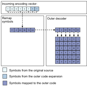
Figure 8: Decoding process in a Fulcrum outer decoder. The inner code encoding vector is mapped directly back to the outer field. Then, a standard decoder can be used to decode the data.

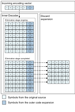
(a)

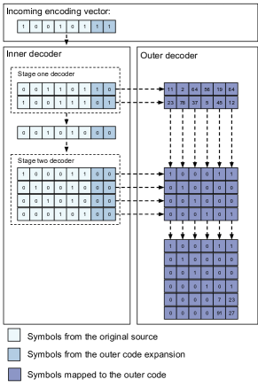
(b)

Figure 9: Examples of Fulcrum’s (a) inner decoder and (b) combined decoder. A Fulcrum inner decoder (a) skips the use of the outer code by decoding the entire inner block and then discarding all symbols belonging to the outer expansion. A Fulcrum combined decoder (b) uses a two stage inner decoder to eliminate as much of the contribution of the outer code as possible before mapping the symbol to the outer decoder. It should be noted that this only works in cases where the outer code is systematic.

In order to understand how this works, let us go through the example shown in Fig. 9b. When an encoding vector arrives at a combined decoder, it is first passed to the inner decoder. Internally, the inner decoder is split into two stages. In stage one, we attempt to eliminate the extension added in the outer encoder (these are the symbols that when mapped to the outer decoder will have coding coefficients from the outer field). If stage one successfully eliminates the expansion, the symbol is passed to stage two. In the stage two decoder, we only have linear combinations of original source symbols. These symbols have a trivial encoding vector when mapped to the outer decoder. Once stage one and stage two combined have full rank the stored symbols are mapped to the outer decoder. Notice in Fig. 9b how symbols coming from stage two have coding coefficients $0$ or $1$ require only a few operations to be decoded, whereas the symbols coming from stage one have a dense structure with coding coefficients coming from the outer field, represented by $c_{xy}\in GF(2^{h})$, where $GF(2^{h})$ is the field used for the outer code. After mapping to the outer decoder, the final step is to solve the linear system shown in the lower right of Figure 9b.

VI Performance Results

In the following section, we present performance results obtained by running the different algorithms on various devices as depicted in Table II. For all benchmarks a packet size of 1600 B was used and the outer Fulcrum code is performed over $GF(2^{8})$. We implemented the Fulcrum encoder and the three decoder types in Kodo [40]. The results for the RLNC encoders and decoders in $GF(2)$ (“Binary” in the Figures) and $GF(2^{8})$ (“Binary8” in the Figures) use the current implementation in this library with and without Single Instruction Multiple Data (SIMD) operations for hardware speed up. Performance is evaluated using Kodo’s benchmarks. We assume a systematic outer code structure to compare performance of the three decoder types.

Alias	Device	CPU
N6	Nexus 6	Quad-core 2.7 GHz Krait 450
N9	Nexus 9	Dual-core 2.3 GHz Denver
i5	Intel NUC D54250WYK	Dual-core 2.6 GHz Intel core i5-4250U
i7	Dell latitude E6530	Quad-core 2.7 GHz Intel core i7-3740QM
Rasp v2	Raspberry PI 2 model B V1.1	Quad-core 900MHz ARM Cortex-A7 CPU
S5	Samsung S5	Quad-core 2.5 GHz Krait 400

TABLE II: Measured devices

Figure 10a shows the decoding throughput for the Fulcrum code, with different $r$ and decoder type. This is compared against the performance of an RLNC decoder using $GF(2)$, as this represents the fastest dense code, and an RLNC decoder using $GF(2^{8})$, as this represents a commonly used dense code with the same field size used in the outer code of the Fulcrum schemes and where decoding probability approaches 1 when $n$ packets have been received.

When only the inner code over $GF(2)$ is utilized for decoding in Fulcrum (inner decoder), Fulcrum is similar to RLNC over $GF(2)$. When only the outer code over $GF(2^{8})$ is utilized in Fulcrum (outer decoder), Fulcrum becomes similar to RLNC over $GF(2^{8})$. Thus, in these two cases the decoding throughput for Fulcrum is expected to be equivalent to RLNC over $GF(2)$ and RLNC over $GF(2^{8})$, respectively. This is confirmed and verifies that the decoding implementation performs as expected in these two known cases. The case of the combined decoder is more interesting as it shows the gain over RLNC with $GF(2^{8})$. Not only is the Fulcrum combined decoder always faster compared to RLNC over $GF(2^{8})$, but the performance also approaches that of RLNC over $GF(2)$ as the generation size grows. For $n=1024$ packets, the combined decoder is $20$ times faster than the RLNC over $GF(2^{8})$, but with similar decoding probability.

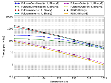
(a)

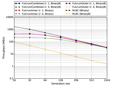
(b)

Figure 10: Processing speed of an i7 without SIMD optimizations for (a) decoding of various Fulcrum decoders compared to RLNC decoders, and (b) encoding of Fulcrum compared to RLNC encoding. The encoding speed of Fulcrum does not depend on the decoder type (combined, inner, or outer).

Figure 10a shows that the combined decoder has some performance dependence for small generation size for different $r$ values, namely, the higher the $r$ the lower the processing speed, but faster than the outer decoder. However, this difference in performance becomes negligible as the number of data packets per generation increases. The reason is that most of the processing effort will be spent decoding in the inner code, and the effect of the $r$ expansion packets is less marked. Decoding speed is usually given a higher priority than the encoding speed, e.g., if there are more decoders than encoders, or because the decoding process tends to be slower than the encoding one. However, encoding speed can be critical in some cases, e.g., a satellite transmitting to an earth station, sensor nodes collecting and sending data to a base station, because there is an inherent constraint on the sender’s computational capabilities or energy. Figure 10b shows the encoding speed compared to the baseline RLNC over $GF(2)$ and $GF(2^{8})$. For the case of $n=16$ packets in the generation, the Fulcrum encoder runs $3.2$x to $6.6$x faster for $r=1$ and $r=4$, respectively, compared to the $GF(2^{8})$ RLNC encoder. As $n$ increases, so does the gain over the RLNC $GF(2^{8})$ and the dependency on the choice of $r$ decreases. For example, at $n=128$ packets the Fulcrum encoder is approximately $14$x faster than the RLNC $GF(2^{8})$ encoder, and for $g=256$ the encoding speed is close to RLNC over $GF(2)$.

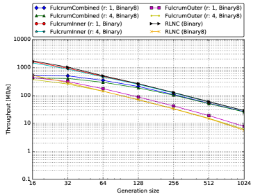
(a)

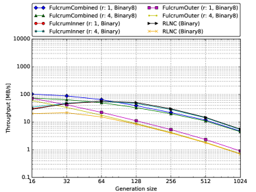
(b)

Figure 11: Processing speed of decoding with SIMD optimizations for (a) the i7 and (b) the N6

Figure 11a studies the effect of SIMD instructions on the performance of the decoders on the i7. This optimization has an effect on operations with $GF(2^{8})$, which means that the RLNC $GF(2)$ decoder and the inner decoder will show no changes from Figure 10a. Figure 11a shows similar trends, but with reduced gains with respect to RLNC over $GF(2^{8})$ as the performance of $GF(2^{8})$ operations are greatly improved. Nonetheless, at $n=128$ the decoding speed is $2.8$ times higher than RLNC $GF(2^{8})$ and close to the performance of RLNC over $GF(2)$.

Figure 11b shows the performance of the decoders with SIMD optimizations on a N6 mobile device. The trends in the N6 are more surprising, as standard RLNC decoders for $GF(2)$ are slower than the Combined Decoders for $n\leq 64$ (up to 3.3 times slower at $n=16$). This gain of the combined decoder is similar when compared to Inner decoders, which use the same algorithm as RLNC $GF(2)$ for decoding purposes. This means that the combined decoder is not only faster than RLNC in $GF(2^{8})$ in the N6, but also faster than RLNC in $GF(2)$ for the small and medium range of $n$. Figure 11b also shows that the Fulcrum outer decoder can also be faster than RLNC $GF(2^{8})$ for $n\leq 64$ packets. Similar trends have been observed for the S5 and the N9, showing that Fulcrum does not require all devices to trade-off speed for performance (or vice-versa) but can provide better performance in both domains.

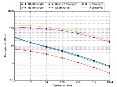
(a)

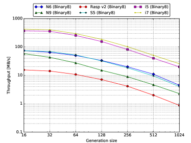
(b)

Figure 12: Processing speed of Combined Decoder (a) without SIMD and (b) with SIMD for different devices

Finally, Figures 12a and 12b show the performance of the combined decoder on various commercial devices without and with SIMD optimizations, respectively. The use of SIMD results two- to four-fold speed ups for all devices for low $n$. However, we observe that the benefit of SIMD is more marked for mobile devices at high $n$ (up to five times the speed up), while for desktops the gains over no SIMD have essentially dissapeared. This does not mean that SIMD in desktops is not improving computation of $GF(2^{8})$, but rather that the main limitation becomes the processing of $GF(2)$ operations at high speeds. More important is the fact that mobile devices, which are more energy and computationally limited, can benefit significantly and over a large range of $n$ from the combination of Fulcrum and the use of apropriate SIMD instructions.

VII Conclusions

This paper presents Fulcrum network codes, an advanced network code structure that preserves RLNC’s ability to recode seamlessly in the network while providing key mechanisms for practical deployment of network coding. Fulcrum addresses several of the standing practical problems with existing RLNC codes and rateless codes, by employing a concatenated code design. This concatenated code design provides our solution with a highly flexible, tunable and intuitive design. This paper describes in detail the design of Fulcrum network codes and its practical benefits over previous network coding designs and it provides mathematical analysis on the performance of Fulcrum network codes under a wide range of conditions and scenarios. The paper also presents a first implementation of Fulcrum in the Kodo C++ network coding library as well as benchmarking its performance to high-performance RLNC encoder and decoders.

Our throughput benchmarks show that Fulcrum provides much higher encoding/decoding processing speed compared to RLNC $GF(2^{8})$. In fact, the processing speeds approach those of RLNC $GF(2)$ as the generation size grows. More importantly, Fulcrum can maintain the decoding probability performance of RLNC $GF(2^{8})$ at the same time that the processing speed is increased by up to a factor of $20$ in some scenarios with our initial implementation. Furthermore, the trade-off between coding processing speed and decoding probability can easily be adjusted using the outer code expansion $r$ to meet the requirements of a given application.

Fulcrum solves several standing problems for existing RLNC codes. First, it enables an easily adjustable trade-off between coding throughput and decoding probability. Second, it provides a higher coding processing speed when compared to the existing RLNC codes in use. Third, it reduces the overhead associated with the coding vector representation, necessary for recoding, while maintaining a high decoding probability. Fourth, it reduces the type of operations and logic that the network needs to support while allowing end-to-end devices to tailor their desired service and performance, making a key step to widely deploying network coding in practice. This has an added advantage of allowing the network to support future designs seamlessly and naturally providing backwards compatibility.

Given these advantages, Fulcrum is particularly well suited for a wide range of scenarios, including (i) distributed storage, where the reliability requirements are high and many storage units are in use; (ii) wireless (mesh) networks, where the packet size is typically small, which results in large generation sizes when large file are transmitted; (iii) heterogeneous networks, since Fulcrum supports different decoding options for (computationally) strong and weak decoders; (iv) wireless sensor networks, where the packet sizes are small requiring small overhead and also the devices are energy- and computationally-limited. Future work will study optimal solutions to use Fulcrum’s structure to spread the complexity over the network.

References

- [1] R. Ahlswede, N. Cai, S.-Y. R. Li, , and R. W. Yeung, “Network information flow,” IEEE Trans. on Info. Theory, vol. 46, no. 4, 2000.
- [2] P. Elias, A. Feinstein, and C. E. Shannon, “A note on the maximum flow through a network,” IRE Transactions on Information Theory, vol. 2, no. 4, pp. 117–119, 1956.
- [3] S.-Y. Li, R. W. Yeung, and N. Cai, “Linear network coding,” IEEE Trans. on Info. Theory, vol. 49, no. 2, pp. 371–381, 2003.
- [4] T. Ho, M. Medard, R. Koetter, D. R. Karger, M. Effros, J. Shi, and B. Leong, “A random linear network coding approach to multicast,” IEEE Trans. on Info. Theory, vol. 52, no. 10, pp. 4413–4430, 2006.
- [5] F. Zhao and M. Médard, “On analyzing and improving cope performance,” in Info. Theory and App. Workshop (ITA), San Diego, CA, USA, Jan. 2010, pp. 1–6.
- [6] M. Hundebøll, J. Ledet-Pedersen, S. Rein, and F. H. Fitzek, “Comparison of analytical and measured performance results on network coding in ieee 802.11 ad-hoc networks,” in Proc. of 76th IEEE Vehicular Tech. Conf., 2012.
- [7] M. Nistor, D. E. Lucani, T. T. V. Vinhoza, R. A. Costa, and J. Barros, “On the delay distribution of random linear network coding,” IEEE Journal on Sel. Areas in Comm., vol. 29, no. 5, pp. 1084–1093, 2011.
- [8] H. Seferoglu and A. Markopoulou, “Video-aware opportunistic network coding over wireless networks,” IEEE Journal on Sel. Areas in Comm., vol. 27, no. 5, pp. 713–728, 2009.
- [9] A. Dimakis, K. Ramchandran, Y. Wu, and C. Suh, “A survey on network codes for distributed storage,” Proceedings of the IEEE, vol. 99, no. 3, pp. 476–489, 2011.
- [10] C. Gkantsidis, J. Miller, and P. Rodriguez, “Comprehensive view of a live network coding p2p system,” in Proceedings of the 6th ACM SIGCOMM conference on Internet measurement, ser. IMC ’06, NY, USA, 2006, pp. 177–188.
- [11] S. Katti, H. Rahul, W. Hu, D. Katabi, M. M dard, and J. Crowcroft, “Xors in the air: practical wireless network coding,” IEEE/ACM Transactions on Networking, vol. 16, no. 3, pp. 497–510, 2006.
- [12] M. V. Pedersen, J. Heide, F. H. P. Fitzek, and T. Larsen, “Pictureviewer - a mobile application using network coding,” in European Wireless Conference (EW), 2009, pp. 151–156.
- [13] P. Vingelmann, F. H. P. Fitzek, M. V. Pedersen, J. Heide, and H. Charaf, “Synchronized multimedia streaming on the iphone platform with network coding,” IEEE Communications Magazine, vol. 49, no. 6, pp. 126–132, 2011.
- [14] J. Heide, M. V. Pedersen, F. H. P. Fitzek, and M. Medard, “On code parameters and coding vector representation for practical rlnc,” in IEEE Int. Conf. on Comm. (ICC), 2011, pp. 1–5.
- [15] J. Heide, M. V. Pedersen, F. H. P. Fitzek, and T. Larsen, “Network coding for mobile devices - systematic binary random rateless codes,” in IEEE Int. Conf. on Comm. (ICC) Workshops, 2009, pp. 1–6.
- [16] A. Paramanathan, M. V. Pedersen, D. E. Lucani, F. H. P. Fitzek, and M. Katz, “Lean and mean: network coding for commercial devices,” IEEE Wireless Communications, vol. 20, no. 5, pp. 54–61, October 2013.
- [17] M. Nistor, D. E. Lucani, and J. Barros, “A total energy approach to protocol design in coded wireless sensor networks,” in Int. Symp. on Net. Cod. (NetCod),, 2012, pp. 31–36.
- [18] D. E. Lucani, M. Medard, and M. Stojanovic, “Random linear network coding for time-division duplexing: Field size considerations,” in IEEE Global Telecom. Conf. (GLOBECOM), 2009, pp. 1–6.
- [19] J. G. D. Forney, Concatenated Codes. Cambridge, MA: M.I.T. Press, 1966.
- [20] A. Shokrollahi, “Raptor codes,” IEEE Trans. on Info. Theory, vol. 52, no. 6, pp. 2551–2567, 2006.
- [21] J. P. Thibault, W. Y. Chan, and S. Yousefi, “A family of concatenated network codes for improved performance with generations,” Journal of Communications and Networks, vol. 10, no. 4, pp. 384–395, 2008.
- [22] S. W. Kim, “Concatenated network coding for large-scale multi-hop wireless networks,” in IEEE Wireless Comm. and Networking Conf. (WCNC), 2007, pp. 985–989.
- [23] Y. Yin, R. Pyndiah, and K. Amis, “Performance of random linear network codes concatenated with reed-solomon codes using turbo decoding,” in 6th Int. Symp. on Turbo Codes and Iterative Information Proc. (ISTC), 2010, pp. 132–136.
- [24] V. Skachek, O. Milenkovic, and A. Nedic, “Hybrid noncoherent network coding,” IEEE Trans. on Info. Theory, vol. 59, no. 6, pp. 3317–3331, June 2013.
- [25] N. Thomos and P. Frossard, “Toward one symbol network coding vectors,” IEEE Comm. Letters, vol. 16, no. 11, pp. 1860–1863, 2012.
- [26] J. Heide, M. V. Pedersen, F. H. Fitzek, and M. Médard, “A perpetual code for network coding,” in IEEE Veh. Tech. Conf. (VTC) - Wireless Networks and Security Symposium, 2013.
- [27] S. Feizi, D. E. Lucani, and M. Medard, “Tunable sparse network coding,” in Int. Zurich Seminar on Communications (IZS), Feb. 2012, pp. 107–110.
- [28] R. Prior, D. E. Lucani, Y. Phulpin, M. Nistor, and J. Barros, “Network coding protocols for smart grid communications,” IEEE Trans. on Smart Grid, 2014.
- [29] M.-H. Lee and Y. L. Borissov, “On jacket transforms over finite fields,” in IEEE Int. Symp. on Info. Theory (ISIT), June 2009, pp. 2803–2807.
- [30] J. P. Vilela, L. Lima, and J. Barros, “Lightweight security for network coding,” in IEEE Int. Conf. on Comm. (ICC), 2008, pp. 1750–1754.
- [31] P. Zhang, Y. Jiang, C. Lin, Y. Fan, and X. Shen, “P-coding: Secure network coding against eavesdropping attacks,” in IEEE INFOCOM, 2010, pp. 1–9.
- [32] J. Justesen and T. Hoeholdt, A Course In Error-Correcting Codes, ser. EMS Textbooks in Math. EMS Pub. House, 2004.
- [33] F. MacWilliams and N. Sloane, The Theory of Error Correcting Codes, ser. North-Holland mathematical library. North-Holland Publishing Company, 1977, no. del 1–2.
- [34] F. Hernando, M. E. O’Sullivan, E. Popovici, and S. Srivastava, “Subfield-subcodes of generalized toric codes,” in 2010 IEEE International Symposium on Information Theory (ISIT), June 2010, pp. 1125–1129.
- [35] L. S. Heath and N. A. Loehr, “New algorithms for generating conway polynomials over finite fields,” Journal of Symbolic Computation, vol. 38, no. 2, pp. 1003 – 1024, 2004.
- [36] Qualcomm. (2013, Dec.) Raptorq - the superior fec technology. [Online]. Available: http://www.qualcomm.com/media/documents/raptorq-data-sheet
- [37] S. Feizi, D. E. Lucani, C. W. Sorensen, A. Makhdoumi, and M. Medard, “Tunable sparse network coding for multicast networks,” in Int. Symp. on Network Coding (NetCod), June 2014, pp. 1–6.
- [38] D. J. C. Mackay, Information Theory, Inference & Learning Algorithms. Cambridge University Press, June 2002.
- [39] Steinwurf ApS. (2012) Kodo git repository on github. Http://github.com/steinwurf/kodo.
- [40] M. V. Pedersen, J. Heide, and F. Fitzek, “Kodo: An open and research oriented network coding library,” Lecture Notes in Computer Science, vol. 6827, pp. 145–152, 2011.