Reducing Clocks in Timed Automata while Preserving Bisimulation

Abstract

Model checking timed automata becomes increasingly complex with the increase in the number of clocks. Hence it is desirable that one constructs an automaton with the minimum number of clocks possible. The problem of checking whether there exists a timed automaton with a smaller number of clocks such that the timed language accepted by the original automaton is preserved is known to be undecidable. In this paper, we give a construction, which for any given timed automaton produces a timed bisimilar automaton with the least number of clocks. Further, we show that such an automaton with the minimum possible number of clocks can be constructed in time that is doubly exponential in the number of clocks of the original automaton.

1 Introducton

Timed automata [AD1] is a formalism for modelling and analyzing real time systems. The complexity of model checking is dependent on the number of clocks of the timed automaton (TA) [AD1, ACD1]. Model checkers use the region graph or a zone graph construction for analysing reachability and other properties in timed automata. These graphs have sizes exponential in the number of clocks of the timed automaton. The algorithms for model checking in turn depend on the sizes of these graphs. Hence it is desirable to construct a timed automaton with the minimum number of clocks that preserves some property of interest (such as timed language equivalence or timed bisimilarity). Here we show that checking the existence of a timed automaton with fewer clocks that is timed bisimilar to the original timed automaton is decidable. Our method is constructive and we provide a 2-EXPTIME algorithm to construct the timed bisimilar automaton with the least possible number of clocks. We also note that if the constructed TA has a smaller number of clocks, then it implies that there exists an automaton with a smaller number of clocks accepting the same timed language.

Related work: In [DY1], an algorithm has been provided to reduce the number of clocks of a given timed automaton. It produces a new timed automaton that is timed bisimilar to the original one. The algorithm detects a set of active clocks at every location and partitions these active clocks into classes such that all the clocks belonging to a class in the partition always have the same value. However, this may not result in the minimum possible number of clocks. The algorithm described in the paper [DY1] works on the timed automaton directly rather than on its semantics. For instance, if a constraint associated with clock $x$ implies a constraint associated with clock $y$, and the conjunction of the two constraints appears on an edge, then the constraint associated with clock $y$ may be eliminated. However, the algorithm of [DY1] does not capture such implication. Also by considering constraints on more than one outgoing edge from a location, e.g. $l_{0}\xrightarrow{a,x\leq 3,\emptyset}l_{1}$ and $l_{0}\xrightarrow{a,x>3,\emptyset}l_{2}$ collectively, we may sometimes eliminate the constraints that may remove some clock. This too has not been accounted for by the algorithm of [DY1].

In a related line of work [Trip1], it has been shown that no algorithm can decide the following two things together.

1. minimality of the number of clocks while preserving the timed language and

2. for the non-minimal case finding a timed language equivalent automaton with fewer clocks.

Also as mentioned earlier, for a given timed automaton, the problem of determining whether there exists another TA with fewer clocks accepting the same timed language is undecidable [Fin1].

Another result appearing in [LLW1] which uses the region-graph construction is the following. A $(C,M)$-automaton is one with $\lvert C\lvert$ clocks and $M$ is the largest integer appearing in the timed automaton. Given a timed automaton $A$, a set of clocks $C$ and an integer $M$, checking the existence of a ($C,M$)-automaton that is timed bisimilar to $A$ is shown to be decidable. The method described there constructs a logical formula called the characteristic formula and checks whether there exists a $(C,M)$-automaton that satisfies it. Further, it is shown that a pair of automata satisfying the same characteristic formula are timed bisimilar. The paper also considers the following problem $P$ and leaves it open.

Does there exist a timed automaton with $|C|$ clocks that is timed bisimilar to $A$?

We solve the following problem $Q$.

Given a timed automaton $A$, construct a timed bisimilar automaton $B$ with the least number of clocks.

Solving the problem $Q$ also solves the problem $P$ and vice versa. If $B$ has say $|C^{\prime}|$ clocks and $|C|\geq|C^{\prime}|$, then the answer to the problem $P$ is in the affirmative. For the problem $P$, if the answer is ‘yes’ for $|C|$ clocks but the answer is ‘no’ for $|C|-1$ clocks, then it is clear that the timed automaton with the minimum possible number of clocks that is timed bisimilar to $A$ can have no less than $\lvert C\lvert$ clocks.

The rest of the paper is organized as follows: in Section 2, we describe timed automata and introduce several concepts that will be used in the paper. We also describe the construction of the zone graph in Section 3 used in reducing the number of clocks. This construction of the zone graph has also been used in [GKNA1] for deciding several timed and time abstracted relations. In Section 4, we discuss our approach in detail along with a few examples. Section LABEL:sec-conc is the conclusion.

2 Timed Automata

Formally, a timed automaton (TA) [AD1] is defined as a tuple $A=(L,Act,l_{0},C,E)$ where $L$ is a finite set of locations, $Act$ is a finite set of visible actions, $l_{0}\in L$ is the initial location, $C$ is a finite set of clocks and $E\subseteq L\>\times\>\mathcal{B}(C)\>\times\>Act\>\times\>2^{C}\>\times\>L$ is a finite set of edges. The set of constraints or guards on the edges, denoted $\mathcal{B}(C)$, is given by the grammar $g::=\;x\bowtie k\>|\>g\wedge g$, where $k\in\mathbb{N}$ and $x\in C$ and $\bowtie\>\in\>\{\leq,<,=,>,\geq\}$. Given two locations $l,l^{\prime}$, a transition from $l$ to $l^{\prime}$ is of the form $(l,g,a,R,l^{\prime})$ i.e. a transition from $l$ to $l^{\prime}$ on action $a$ is possible if the constraints specified by $g$ are satisfied; $R\subseteq C$ is a set of clocks which are reset to zero during the transition.

The semantics of a timed automaton(TA) is described by a timed labelled transition system (TLTS) [LAKJ1]. The timed labelled transition system $T(A)$ generated by $A$ is defined as $T(A)=(Q,Lab,Q_{0},\{\stackrel{{\scriptstyle\alpha}}{{\longrightarrow}}|\alpha\in Lab\})$, where $Q\>=\>\{(l,v)\>|\>l\in L,v\in{\mathbb{R}_{\geq 0}}^{|C|}\}$ is the set of states, each of which is of the form $(l,v)$, where $l$ is a location of the timed automaton and $v$ is a valuation in $|C|$ dimensional real space where each clock is mapped to a unique dimension in this space; $Lab=Act\cup\mathbb{R}_{\geq 0}$ is the set of labels. Let $v_{0}$ denote the valuation such that $v_{0}(x)=0$ for all $x\in C$. $Q_{0}=(l_{0},v_{0})$ is the initial state of $T(A)$. A transition may occur in one of the following ways:
(i) Delay transitions : $(l,v)\stackrel{{\scriptstyle d}}{{\longrightarrow}}(l,v+d)$. Here, $d\in\mathbb{R}_{\geq 0}$ and $v+d$ is the valuation in which the value of every clock is incremented by $d$.
(ii) Discrete transitions : $(l,v)\stackrel{{\scriptstyle a}}{{\longrightarrow}}(l^{\prime},v^{\prime})$ if for an edge $e=(l,g,a,R,l^{\prime})\in\>E$, $v$ satisfies the constraint $g$, (denoted $v\models g$), $v^{\prime}=v_{[R\leftarrow\overline{0}]}$, where $v_{[R\leftarrow\overline{0}]}$ denotes that every clock in $R$ has been reset to 0, while the remaining clocks are unchanged. From a state $(l,v)$, if $v\models g$, then there exists an $a$-transition to a state $(l^{\prime},v^{\prime})$; after this, the clocks in $R$ are reset while those in $C\backslash R$ remain unchanged.

For simplicity, we do not consider annotating locations with clock constraints (known as invariant conditions [HNSY1]). Our results extend in a straightforward manner to timed automata with invariant conditions. In Section 4, we provide the modifications to our method for dealing with location invariants. We now define various concepts that will be used in the rest of the paper.

Definition 1

Let $A=(L,Act,l_{0},E,C)$ be a timed automaton, and $T(A)$ be the TLTS corresponding to $A$.

1. Timed trace: A sequence of delays and visible actions $d_{1}a_{1}d_{2}a_{2}\dots d_{n}a_{n}$ is called a timed trace of the timed automaton $A$ iff there is a sequence of transitions $p_{0}\xrightarrow{d_{1}}p_{1}\xrightarrow{a_{1}}p_{1}^{\prime}\xrightarrow{d_{2}}p_{2}\xrightarrow{a_{2}}p_{2}^{\prime}\cdots\xrightarrow{d_{n}}p_{n}\xrightarrow{a_{n}}p_{n}^{\prime}$ in $T(A)$, where each $p_{i}$ and $p_{i}^{\prime}$, $0\leq i\leq n$ are timed automata states and are of the form $(l,v)$. $p_{0}$ is the initial state of the timed automaton. Given a timed trace $tr=d_{1}a_{1}d_{2}a_{2}\dots d_{n}a_{n}$, $untime(tr)$ denotes its projection on $Act$, i.e. $untime(tr)=a_{1}a_{2}\dots a_{n}$.

2. Zone and difference bound matrix (DBM): A zone $Z$ is a set of valuations $\{v\in\mathbb{R}_{\geq 0}^{|C|}\mid v\models\beta\}$, where $\beta$ is of the form $\beta::=\;x\bowtie k\>|\>x-y\bowtie k\>|\>\beta\wedge\beta$, $k$ is an integer, $x,y\in C$ and $\bowtie\>\in\>\{\leq,<,=,>,\geq\}$. $Z\!\!\uparrow$ denotes the future of the zone $Z$. $Z\!\!\uparrow=\{v+d\mid v\in Z,d\geq 0\}$ is the set of all valuations reachable from $Z$ by delay transitions. A zone is a convex set of clock valuations. A difference bound matrix is a data structure used to represent zones. A DBM [BM1, Dill1] for a set $C=\{x_{1},x_{2},\dots,x_{n}\}$ of $n$ clocks is an $(n+1)$ square matrix $\Xi$ where an extra variable $x_{0}$ is introduced such that the value of $x_{0}$ is always $0$. An element $\Xi_{ij}$ is of the form $(m_{ij},\prec)$ where $\prec\in\{<,\leq\}$ such that $x_{i}-x_{j}\prec m_{ij}$. Thus an entry $m_{i0}$ denotes the constraint $x_{i}-x_{0}\prec m_{i0}$ which is equivalent to $x_{i}\prec m_{i0}$.

3. Canonical decomposition: Let $\displaystyle{g=\bigwedge_{i=1}^{n}\gamma_{i}\in\mathcal{B}(C)}$, where each $\gamma_{i}$ is an elementary constraint of the form $x_{i}\bowtie k_{i}$, such that $x_{i}\in C$ and $k_{i}$ is a non-negative integer. A canonical decomposition of a zone $Z$ with respect to $g$ is obtained by splitting $Z$ into a set of zones $Z_{1},\dots,Z_{m}$ such that for each $1\leq j\leq m$, and $1\leq i\leq n$, either $\forall v\in Z_{j},v\models\gamma_{i}$ or $\forall v\in Z_{j}$, $v\not\models\gamma_{i}$. For example, consider the zone $Z=x\geq 0\wedge y\geq 0$ and the guard $x\leq 2\wedge y>1$. $Z$ is split with respect to $x\leq 2$, and then with respect to $y>1$, hence into four zones : $x\leq 2\wedge y\leq 1$, $x>2\wedge y\leq 1$, $x\leq 2\wedge y>1$ and $x>2\wedge y>1$. An elementary constraint $x_{i}\bowtie k_{i}$ induces the hyperplane $x_{i}=k_{i}$ in a zone graph of the timed automaton.

4. Zone graph: Given a timed automaton $A=(L,Act,l_{0},C,E)$, a zone graph $\mathcal{G}_{A}$ of $A$ is a transition system $(S,s_{0},Lep,\rightarrow)$, that is a finite representation of $T(A)$. Here $Lep=Act\cup\{\varepsilon\}$. $S\subseteq L\times\mathcal{Z}$ is the set of nodes of $\mathcal{G}_{A}$, $\mathcal{Z}$ being the set of zones. The node $s_{0}=(l_{0},Z_{0})$ is the initial node such that $v_{0}\in Z_{0}$. $(l_{i},Z)\xrightarrow{a}(l_{j},Z^{\prime})$ iff $l_{i}\xrightarrow{g,a,R}l_{j}$ in $A$ and $Z^{\prime}\subseteq([Z\cap g]_{R\leftarrow\overline{0}})\!\!\uparrow$ obtained after canonical decomposition of $([Z\cap g]_{R\leftarrow\overline{0}})$. For any $Z$ and $Z^{\prime}$, $(l_{i},Z)\xrightarrow{\varepsilon}(l_{i},Z^{\prime})$ iff there exists a delay $d$ and a valuation $v$ such that $v\in Z$, $v+d\in Z^{\prime}$ and $(l_{i},v)\stackrel{{\scriptstyle d}}{{\longrightarrow}}(l_{i},v+d)$ is in $T(A)$. Here the zone $Z^{\prime}$ is called a delay successor of zone $Z$, while $Z$ is called the delay predecessor of $Z^{\prime}$. Every node has an $\varepsilon$ transition to itself and the $\varepsilon$ transitions are also transitive. The relation $\xrightarrow{\varepsilon}$ is reflexive and transitive and so is the delay successor relation. We denote the set of delay successor zones of $Z$ by $ds(Z)$. A zone $Z^{\prime}\neq Z$ is called the immediate delay successor of a zone $Z$ iff $Z^{\prime}\in ds(Z)$ and $\forall Z^{\prime\prime}\in ds(Z):Z^{\prime\prime}\neq Z$ and $Z^{\prime\prime}\neq Z^{\prime}$, $Z^{\prime\prime}\in ds(Z^{\prime})$. We call a zone $Z$ corresponding to a location to be a base zone if $Z$ does not have a delay predecessor other than itself. For both $a$ and $\varepsilon$ transitions, if $Z$ is a zone then $Z^{\prime}$ is also a zone, i.e. $Z^{\prime}$ is a convex set.

5. A hyperplane $x=k$ is said to bound a zone $Z$ from above if $\exists v\in Z\>[\>\forall d\in\mathbb{R}_{\geq 0}\>[\>(v+d)(x)\succ k\iff(v+d)(x)\notin Z\>]\>]$, where $\succ\in\{>,\geq\}$. A zone, in general, can be bounded above by several hyperplanes. A hyperplane $x=k$ is said to bound a zone $Z$ fully from above if $\forall v\in Z\>[\>\forall d\in\mathbb{R}_{\geq 0}\>[\>(v+d)(x)\succ k\iff(v+d)(x)\notin Z\>]\>]$. Analogously, we can also say that a hyperplane $x=k$ bounds a zone from below if $\exists v\in Z\>[\>\forall d\in\mathbb{R}_{\geq 0}\>[\>(v-d)(x)\prec k\iff(v-d)(x)\notin Z\>]\>]$, where $\prec\in\{<,\leq\}$. We can also define a hyperplane bounding a zone fully from below in a similar manner.

   When not specified otherwise, in this paper, a hyperplane bounding a zone implies that it bounds the zone from above. A zone $Z$ is bounded above if it has an immediate delay successor zone.

6. Pre-stability: A zone $Z_{1}$ of location $l_{1}$ is pre-stable with respect to a transition $\eta\in Lep$ leading to a zone $Z_{2}$ of location $l_{2}$ if
   i) for $\eta=a\in Act\>:$ $\forall v_{1}\in Z_{1},\exists v_{2}\in Z_{2}$ such that $(l_{1},v_{1})\xrightarrow{a}(l_{2},v_{2})$ or $\forall v_{1}\in Z_{1},\not\!\exists v_{2}\in Z_{2}$ such that $(l_{1},v_{1})\xrightarrow{a}(l_{2},v_{2})$.
   ii) for $\eta=\varepsilon\>:$ $\forall v_{1}\in Z_{1},\exists v_{2}\in Z_{2},\exists d\in\mathbb{R}_{\geq 0}$ such that $(l_{1},v_{1})\xrightarrow{d}(l_{2},v_{2})$ or $\forall v_{1}\in Z_{1}$, $\not\!\exists v_{2}\in Z_{2}$ such that $(l_{1},v_{1})\xrightarrow{d}(l_{2},v_{2})$, for any $d\in\mathbb{R}_{\geq 0}$.
   A zone graph is said to be pre-stable if the zones corresponding to each of the nodes of the zone graph are pre-stable with respect to their outgoing transitions. For example zone $Z_{1}$ in Figure 2 is pre-stable with respect to zone $Z_{4}$, however, $Z_{1}\cup Z_{2}\cup Z_{3}$ is not pre-stable with respect to zone $Z_{4}$ since $\exists v\in Z_{3}$ and hence $v\in Z_{1}\cup Z_{2}\cup Z_{3}$ such that for all $d\in\mathbb{R}_{\geq 0}$, $v+d\notin Z_{4}$.

7. corner point and corner point traces: A corner point of a zone in the zone graph is a state where corresponding to each clock $x$, a hyperplane of the form $x=c$ bounding a zone intersects another hyperplane defining the zone. Considering $M$ to be the largest constant appearing in the constraints or the location invariants of the timed automaton, each coordinate of a corner point is of the form $n,n+\delta$ or $n-\delta$ where $n\in\{0,1,\dots,M\}$ and $\delta$ is a symbolic value for an infinitesimally small quantity. In a zone $Z$, there can be two kinds of corner points, an entry corner point and an exit corner point. For an entry corner point, there is a unique exit corner point, that can be reached from the entry corner point by performing a delay $d$ such that any delay more than $d$ will lead to a state that is in a delay successor zone of $Z$.

   For a zone, it is possible to have a pair of such entry and exit corner points that are not distinct, for example, in Figure 2, in zone $Z_{4}$, the corner point ($x=5+\delta,y=7$) is both an entry as well as an exit corner point, while the corner point ($x=5+\delta,y=5+\delta$) is another entry corner point for the same zone $Z_{4}$ and the corresponding exit corner point is $(x=7,y=7)$. If the entry and the exit corner points are distinct, then a non-infinitesimally small delay can be performed from the entry corner point to reach the corresponding exit corner point whereas an infinitesimally small delay from the exit corner point causes it to evolve into an entry corner point of the immediate delay successor zone. A zone that is not bounded above does not have any exit corner point.

   For an entry corner point, the corresponding exit corner point is the next delay corner point whereas for an exit corner point, the entry corner point in the immediate delay successor zone is the next delay corner point.

   Let $c_{1}$ and $c_{2}$ be constraints of the form $x\succ k_{1}$ and $y\prec k_{2}$ respectively, where $k_{1},k_{2}\in\{0,1,\dots,M\}$ and $\succ\>\in\>\{>,\geq\}$ and $\prec\>\in\>\{<,\leq\}$.

   We consider delays of the form $d_{c_{1},c_{2}}$ and $d_{c_{2},c_{1}}$. $d_{c_{1},c_{2}}$ is the delay made from an entry corner point to reach an exit corner point while $d_{c_{2},c_{1}}$ is the delay made from the exit corner point to reach an entry corner point of a delay successor zone. For example, the delay $d_{x\geq 5,y<7}$ denotes a delay made from a state $p^{\prime}$ with $p^{\prime}(x)=5$ and after making this delay it evolves to state $p^{\prime\prime}$ such that $p^{\prime\prime}(y)=7-\delta$. Delays of the form mentioned above are called corner point delays or cp-delays.

   A corner point trace (cp-trace) is a timed trace ending at a corner point through delays and visible actions such that each delay takes the trace from one corner point to the next delay corner point. All the delay actions present in a corner point trace are cp-delays.

We create a zone graph such that for any location $l$, the zones $Z$ and $Z^{\prime}$ of any two nodes $(l,Z)$ and $(l,Z^{\prime})$ in the zone graph are disjoint and all zones of the zone graph are pre-stable. This zone graph is constructed in two phases in time exponential in the number of the clocks. The first phase performs a forward analysis of the timed automaton while the second phase ensures pre-stability in the zone graph. The forward analysis may cause a zone graph to become infinite [BBFL1]. Several kinds of abstractions have been proposed in the literature [DT1, BBFL1, BBLP1] to make the zone graph finite. We use location dependent maximal constants abstraction [BBFL1] in our construction. In phase 2 of the zone graph creation, the zones are further split to ensure that the resultant zone graph is pre-stable.

Some approaches for preserving convexity and implementing pre-stability have been discussed in [TY1]. As an example, consider the timed automaton in Figure 2. The pre-stable zones of location $l_{1}$ are shown in the right side of the figure. In this paper, from now on, unless stated otherwise, zone graph will refer to this form of the pre-stable zone graph that is described above. An algorithmic procedure for the construction of the zone graph is given in [GKNA1].

A relation $\mathcal{R}\subseteq Q\times Q$ is a timed simulation relation if the following conditions hold for any two timed states $(p,q)\in\mathcal{R}$.
$\forall$ $a\in Act$, $p\xrightarrow{a}p^{\prime}\implies\exists q^{\prime}$ : $q\xrightarrow{a}q^{\prime}$ and $(p^{\prime},q^{\prime})\in\mathcal{R}$ and
$\forall d\in\mathbb{R}_{\geq 0}$, $p\xrightarrow{d}p^{\prime}\implies\exists q^{\prime}$ : $q\xrightarrow{d}q^{\prime}$ and $(p^{\prime},q^{\prime})\in\mathcal{R}$.
A timed bisimulation relation is a symmetric timed simulation. Two timed automata are timed bisimilar if and only if their initial states are timed bisimilar. Using a product construction on region graphs, timed bisimilarity for timed automata was shown to be decidable in EXPTIME [Cer1]. In [WL1], a product construction on zone graph was used for deciding timed bisimulation relation for timed automata.

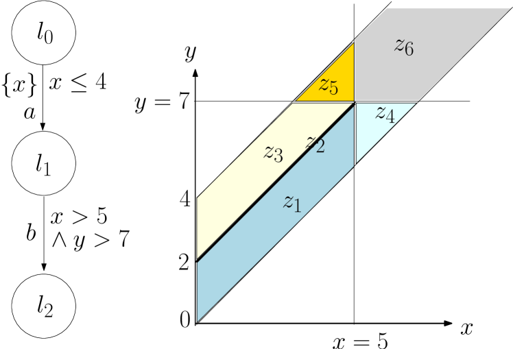
Figure 1: a timed automaton and the zones for location $l_{1}$

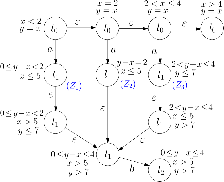
Figure 2: zone graph for the TA in Figure 2

3 Zone Graph

Algorithm 1 Construction of Zone Graph
Input: Timed automaton $A$
Output: Zone graph corresponding to $A$

1:Calculate $max_{x}^{l}$ for each location $l\in L$ and each clock $x\in C$. $\triangleright$ This is required for abstraction to ensure finite number of zones in the zone graph.

2:Initialize $Q$ to an empty queue.

3:$Enqueue(Q,\langle l_{0},\emptyset\rangle)$. $\triangleright$ Every element is a pair consisting of a location and its parent

4:$successors\_added=false$. $\triangleright$ flag set to true whenever successors of a location are added to $Q$

5:while Q not empty do

6:    $\langle l,l_{p}\rangle=dequeue(Q)$

7:    if $l_{p}\neq\emptyset$ then,

8:         For the edge $l_{p}\xrightarrow{g,a,R^{\prime}}l$ in $A$, for each existing zone $Z_{l_{p}}$ of $l_{p}$, create the zone $Z=(Z_{l_{p}}\uparrow\cap\>g_{[R^{\prime}\leftarrow\overline{0}]})$ of $l$, when $Z\neq\emptyset$.

9:         Abstract each of the newly created zones if necessary and for any newly created zone $Z$, for location $l$, if $\exists Z_{1}$ of same location such that $Z\cap Z_{1}\neq\emptyset$, then merge $Z$ and $Z_{1}$.

10:         Update edges from zones of $l_{p}$ to zones of $l$ appropriately.

11:         If a new zone of $l$ is added or an existing zone of $l$ is modified for all successors $l_{j}$ of $l$, enqueue $\langle l_{j},l\rangle$ to Q.

12:         $successors\_added:=true$.

13:    end if

14:    $new\_zone\_l:=true$. $\triangleright$ flag set to false when the canonical decomposition does not produce further zones

15:    while $new\_zone\_l$ do

16:         Split the existing zones $Z$ of $l$ based on the canonical decomposition of the guards on the outgoing edges of $l$ $\triangleright$ It is not always necessary for a split to happen.

17:         For every zone $Z$ of $l$, consider $Z\uparrow$ and split it further based on the canonical decomposition of the guards on the outgoing edges of $l$ $\triangleright$ Note that the zones created from this split are convex.

18:         Abstract each of the newly created zones if necessary and update edges appropriately.

19:         if new zones are not created then set $new\_zone\_l$ to $false$.

20:         end if

21:    end while

22:    if any new zones of $l$ are created or any existing zones of $l$ are modified due to the canonical decomposition of the outgoing edges of $l$ and $successors\_added=false$ then

23:         for all the successor locations $l_{j}$ of $l$ to Q, enqueue $\langle l_{j},l\rangle$ to Q.

24:    end if

25:end while

26:/* Phase 2 : In this phase, pre-stability is enforced */

27:$new\_zone=true$

28:while $new\_zone$ do

29:    $new\_zone=false$

30:    for all edges $l_{i}\xrightarrow{g,a,R^{\prime}}l_{j}$ do

31:         for all pairs of zones $Z_{lik}$, $Z_{ljm}$ such that $Z_{lik}\xrightarrow{\alpha}Z_{ljm}$ is an edge in the zone graph where $\alpha\in Act\cup\mathbb{R}_{\geq 0}$ do

32:             if $Z_{lik}$ is not pre-stable with respect to $Z_{ljm}$, then Split $Z_{lik}$ to make it pre-stable with respect to $Z_{ljm}$. $\triangleright$ Note that this split still maintains convexity of $Z_{lik}$ since the zone is split entirely along an axis that is parallel to the diagonal in the $\lvert C\lvert$-dimensional space.

33:                 $new\_zone:=true$

34:                 Update the incoming and the outgoing edges for the newly created zones.

35:             end if

36:         end for

37:    end for

38:end while

The detailed algorithm for creating the zone graph has been described in Algorithm 1 and consists of two phases, the first one being a forward analysis of the timed automaton while the second phase ensures pre-stability in the zone graph. The presence of an edge to a location $l^{\prime}$ in the timed automaton does not imply that the the action of the edge can be performed or location $l^{\prime}$ is reachable. For an edge $l\xrightarrow{g,a,R}l^{\prime}$, if for all zones $Z$ of $l$, $Z\cap g=\emptyset$, then action $a$ cannot be performed at $l$ and $l^{\prime}$ cannot be reached at $l$. Such edges can be removed from the timed automaton. For a location $l^{\prime}$, if the actions corresponding to none of the incoming edges can be performed, then the location $l^{\prime}$ is unreachable and it can be removed along with its incoming and outgoing transitions.

The set of valuations for every location is initially split into zones based on the canonical decomposition of its outgoing transition.

After phase 2, pre-stability ensures the following: For a node $(l,z)$ in the zone graph, with $v\in z$, for a timed trace $tr$, if $(l,v)\xrightarrow{tr}(l^{\prime\prime},v^{\prime\prime})$, with $v^{\prime\prime}\in z^{\prime\prime}$, then $\forall v^{\prime}\;{}\mbox{in}\;z$, $\exists tr^{\prime}.(l,v^{\prime})\xrightarrow{tr^{\prime}}(l^{\prime\prime},\tilde{v})$, with $untime(tr^{\prime})=untime(tr)$ and $\tilde{v}\in z^{\prime\prime}$. According to the construction given in algorithm 1, for a particular location of the timed automaton, the zones corresponding to any two nodes are disjoint. Convexity of the zones and pre-stability property together ensure that a zone with elapse of time is intercepted by a single hyperplane of the form $x=h$, where $x\in C$ and $h\in\mathbb{N}$. This is stated formally in Lemma 1. Some approaches for preserving convexity and implementing pre-stability have been discussed in [TY1]. As an example consider the timed automaton in Figure 2. The zones corresponding to location $l_{1}$ as produced through algorithm 1 are shown in the right side of the figure.

For a state $q\in T(A)$, $\mathcal{N}(q)$ represents the node of the zone graph with the same location as that of $q$ such that the zone corresponding to $\mathcal{N}(q)$ includes the valuation of $q$. We often say that a state $q=(l,v)$ is in node $s=(l,Z)$ to indicate that $v\in Z$. For two zone graphs, $\mathcal{G}_{A_{1}}=(S_{1},s_{0},Lep,\rightarrow_{1})$, $\mathcal{G}_{A_{2}}=(S_{2},s_{0}^{\prime},Lep,\rightarrow_{2})$ and a relation $\mathcal{R}\subseteq S_{1}\times S_{2}$, $\mathcal{G}_{A_{1}}\>\mathcal{R}\>\mathcal{G}_{A_{2}}$ iff $(s_{p},s_{q})\in\mathcal{R}$. An $\varepsilon$ transition represents a delay $d\in\mathbb{R}_{\geq 0}$.

3.1 Creating pre-stable zones

We describe below a procedure for splitting a zone $Z_{1}$ into a set $\mathcal{Z}_{1}$ of zones w.r.t a zone $Z_{2}$ such that the following properties are satisfied.

1. Each zone $Z_{i}$ in $\mathcal{Z}_{1}$ should either be a subset of $Z_{2}$ or disjoint from $Z_{2}$.

2. The DBMs in $\mathcal{Z}_{1}$ are mutually exclusive and disjoint.

3. The union of the DBMs in $\mathcal{Z}_{1}$ is $Z_{1}$.

A naive approach would be to populate $\mathcal{Z}_{1}$ with two DBMs, namely the (set) intersection and (set) difference of $Z_{1}$ with $Z_{2}$. This ensures that the properties 1, 2 and 3 hold. However, while the intersection of two DBMs is always a DBM, this cannot be said for their difference. Thus, we seek to refine our process by replacing the difference of $Z_{1}$ and $Z_{2}$ with some DBMs which are mutually exclusive and which cover the difference of $Z_{1}$ and $Z_{2}$, so that properties 2 and 3 continue to hold.

One naive way to achieve this is to initially populate $\mathcal{Z}_{1}$ with only $Z_{1}$, and then iterate through all the elementary clock constraints $c_{ij}$ of $Z_{2}$. The element $m_{ij}$ in the DBM is a constraint of the form $x_{i}-x_{j}<k$ or $x_{i}-x_{j}\leq k$. In each iteration, we replace each DBM in $\mathcal{Z}_{1}$ with two DBMs, namely its intersection and difference with $c_{ij}$. Note that the complement of an elementary clock constraint is always an elementary clock constraint and thus the difference can be calculated by simply taking the intersection with the complement of the elementary constraint, which implies that both the intersection and the difference considering a single elementary constraint as above are DBMs. Of course, some of the DBMs thus produced may be empty, and we do not add these to $\mathcal{Z}_{1}$. The theoretical bound on the number of DBMs in $\mathcal{Z}_{1}$ at the end is $2^{\mbox{(number of elementary clock constraints in dbm2)}}$, that is, $2^{O((n+1)^{2})}$. The term $(n+1)^{2}$ comes from the fact that there are $(n+1)^{2}$ entries in $Z_{2}$ each of which is an elementary clock constraint. The above exponential bound is because of the fact that, in the worst case, we double the number of DBMs in $\mathcal{Z}_{1}$ in each iteration. This leaves us with a set of mutually exclusive zones which satisfies properties 1, 2 and 3.

However, this is inefficient in that it generates too many zones. So, we refine the process of iterating through the elementary clock constraints $c_{ij}$. We start with an empty $\mathcal{Z}_{1}$ and a pointer which initially points to $Z_{1}$. At each iteration, we evaluate the intersection of $c_{ij}$ and the zone pointed to by the pointer and also their difference which too is a zone since the difference is calculated by taking the intersection with the complement of $c_{ij}$. The pointer is then updated to point to the intersection DBM, while the difference DBM is added to $\mathcal{Z}_{1}$. This procedure continues until all the $c_{ij}$ have been seen. In the end, if the pointer’s target is non-empty, we add it to $\mathcal{Z}_{1}$. At this point, the zones in $\mathcal{Z}_{1}$ still cover $Z_{1}$ and also satisfy properties 1 and 2. This method leads to a maximum of one zone being added to $\mathcal{Z}_{1}$ for each $c_{ij}$, and one zone being added at the end, which gives us a maximum of $O((n+1)^{2}+1)$ zones in $\mathcal{Z}_{1}$.

Algorithm 2 describes the procedure mentioned above formally.

Algorithm 2 This algorithm returns the intersection and the difference of two zones.
Input: Two zones $Z_{1}$ and $Z_{2}$
Output: i) $Z$ which is $Z_{1}\cap Z_{2}$ and ii) $\mathcal{Z}_{1}$, a set of zones whose union is $Z_{1}-Z_{2}$

1:$Z:=Z_{1}\cap Z_{2}$

2:$\mathcal{Z}_{1}:=\emptyset$, $p:=Z_{1}$ $\triangleright$ $p$ is a pointer pointing to a zone.

3:for all $i\in[0,n]$ do

4:    for all $j\in[0,n]$ do

5:         Let $c_{ij}$ be the constraint $x_{i}-x_{j}\prec m_{ij}$, where $(m_{ij},\prec)$ is the corresponding entry in the DBM of $Z_{2}$.

6:         Let $\overline{c_{ij}}$ be the complement of the constraint $c_{ij}$.

7:         $Z_{11}:=p\cap c_{ij}$, $Z_{12}:=p\cap\overline{c_{ij}}$

8:         if $Z_{12}\neq\emptyset$ then

9:             $\mathcal{Z}_{1}:=\mathcal{Z}_{1}\cup Z_{12}$

10:         end if

11:         if $Z_{11}\neq\emptyset$ then

12:             $p:=Z_{11}$

13:         end if

14:    end for

15:end for

16:if $Z_{11}\neq\emptyset$ then

17:    $\mathcal{Z}_{1}=\mathcal{Z}_{1}\cup Z_{11}$

18:end if

Pre-stability is ensured corresponding to both delay and discrete transitions in the zone graph.

• Pre-stabilizing zones corresponding to delay transitions: Consider two nodes in the zone graph $(l,Z)\xrightarrow{\varepsilon}(l,Z^{\prime})$ such that $Z$ is not pre-stable w.r.t $Z^{\prime}$. The procedure involves splitting $Z$ w.r.t $Z^{\prime}\!\!\downarrow$ such that each newly created zones obtained by splitting $Z$ is pre-stable w.r.t. $Z^{\prime}$.

  We follow the procedure given in Algorithm 2 to split a zone $Z$ w.r.t the zone $Z^{\prime}$.

• Pre-stabilizing zones corresponding to discrete transitions in the zone graph: Consider two nodes in the zone graph $(l,Z)\xrightarrow{a}(l^{\prime},Z^{\prime})$ such that $a\in Act$ and $Z$ is not pre-stable w.r.t $Z^{\prime}$. The method involving the pre-stabilization operation is similar to the $Pre_{e}(Z^{\prime})$ operator used in backward analysis of the timed automaton, where $e$ is an edge between say location $l$ and $l^{\prime}$ of the timed automaton and $Z^{\prime}$ is a zone of $l^{\prime}$. Formally for an edge $l\xrightarrow{g,a,R}l^{\prime}$ $Pre_{e}(Z^{\prime})$ is defined as the following:

  $Pre_{e}(Z^{\prime})=\{v\in\mathbb{R}_{\geq 0}^{\lvert C\lvert}\ \lvert\exists v^{\prime}\in Z^{\prime},\>\exists t\in\mathbb{R}_{\geq 0}\mbox{ such that }v+t\models g\mbox{ and }$

  $[R\leftarrow 0](v+t)=v^{\prime}\}$

  Let $[\![R=0]\!]$ denotes the set of all clock valuations $v$ such that $v(x)=0$ when $x\in R$ and $v(x)\in\mathbb{R}_{\geq 0}$ when $x\notin R$. $v(x)$ denotes the valuation of clock $x$. In our case, we define the zone $\widehat{Z^{\prime}}$ as follows:
  $\widehat{Z^{\prime}}=[R\leftarrow 0]^{-1}(Z^{\prime}\cap[\![R=0]\!])$. Now $Z$ is split w.r.t $\widehat{Z^{\prime}}$ following Algorithm 2 that makes all the newly created zones pre-stable w.r.t $Z^{\prime}$.

The following lemma states an important property of the zone graph which will further be used for clock reduction.

Lemma 1

Pre-stability ensures that if the zone $Z$ in any node $(l,Z)$ in the zone graph is bounded above, then it is bounded fully from above by a hyperplane $x=h$, where $x\in C$ and $h\in\mathbb{N}$.

Proof

We show the proof for two clocks. The same argument holds for arbitrary number of clocks. Consider a $\lvert C\lvert$ dimensional zone $Z$. Since $\lvert C\lvert=2$, a zone $Z$ that is bounded above is of the form $k_{xy_{2}}\prec x-y\prec k_{xy_{1}}$, $k_{x_{1}}\prec x\prec k_{x_{2}}$ and $k_{y_{1}}\prec y\prec k_{y_{2}}$, where $x$ and $y$ are the two clocks, $\prec\in\{<,\leq\}$. Let $Z$ be bounded above by two hyperplanes $x=k_{x_{2}}$ and $y=k_{y_{2}}$. As can be seen from Figure 3, there are two zones $Z_{1}$ and $Z_{2}$ such that $Z_{1}$ is defined by the inequations $x-y\prec k_{xy_{1}}$, $k_{x_{2}}\prec x$ and $y\prec k_{y_{2}}$, while $Z_{2}$ is defined as $k_{xy_{2}}\prec x-y$, $x\prec k_{x_{2}}$ and $k_{y_{2}}\prec y$. Making $Z$ pre-stable will divide it into two parts:

• $Z^{\prime}$ defined by the inequations $k_{x_{2}}-k_{y_{2}}\prec x-y\prec k_{xy_{1}}$, $k_{x_{1}}\prec x\prec k_{x_{2}}$ and $k_{y_{1}}\prec y$ and

• $\widehat{Z}$ define by the inequations $k_{xy_{2}}\prec x-y\prec k_{x_{2}}-k_{y_{2}}$, $k_{x_{1}}\prec x$ and $y\prec k_{y_{2}}$

$Z^{\prime}$ is bounded fully from above by the hyperplane $k_{x_{2}}$ while $\widehat{Z}$ is bounded fully from above by the hyperplane $k_{y_{2}}$. Note that the inequations defining the zones $Z^{\prime}$ and $\widehat{Z}$ may vary depending on the relation among the various constants $k_{xy_{1}},k_{xy_{2}},k_{x_{1}},k_{x_{2}},k_{y_{1}}$ and $k_{y_{2}}$. In all cases, pre-stability will ensure that there exists a single hyperplane that fully bounds a zone from above.

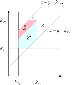
Figure 3: For every zone, there exists a hyperplane that bounds it fully from above in a pre-stable zone graph

4 Clock Reduction

Unlike the method described in [DY1], which works on the syntactic structure of the timed automaton, we use a semantic representation as given by the zone graph described in Section 2 to capture the behaviour of the timed automaton. This helps us to reduce the number of clocks in a more effective way. For a given TA $A$, we first describe a sequence of stages to construct a TA $A_{4}$ that is timed bisimilar to $A$. Later we prove the minimality in terms of the number of clocks for the TA $A_{4}$. The operations involved in our procedure use a difference bound matrix representation of the zones. The following are important considerations in reducing the number of clocks.

• There may be some clock constraints on an edge of the TA that are never enabled. Such edges and constraints may be removed. (Stage 1)

• Splitting some locations may lead to a reduction in the number of the clocks. (Stage 2)

• At some location, some clocks whose values may be expressed in terms of other clock values, may be removed. (Stage 2)

• Two or more constraints on edges outgoing from a location when considered collectively may lead to the removal of some constraints. (Stage 3)

• An efficient way of renaming the clocks across all locations can reduce the total number of clocks further. (Stage 4)

Given a TA $A$, we apply the above operations in sequence to obtain the TA $A_{4}$. These operations are detailed below.

Stage 1: Removing unreachable edges and associated constraints: This stage involves creating the pre-stable zone graph of the given timed automaton, as described in Section 2. As mentioned previously in that section, the edges and their associated constraints that are never enabled in an actual transition are removed while creating the zone graph. Suppose there is an edge $l_{i}\xrightarrow{g,a,R}l_{j}$ in $A$ but in the zone graph, a corresponding transition of the form $(l_{i},Z)\xrightarrow{a}(l_{j},Z^{\prime})$ does not exist. Line 8 in Algorithm 1 also illustrates this. This implies that the transition $l_{i}\xrightarrow{g,a,R}l_{j}$ is never enabled and hence is removed from the timed automaton. Since the edges that do not affect any transition get removed during this stage, we have the following lemma trivially.

Lemma 2

The operations in stage 1 produce a timed automaton $A_{1}$ that is timed bisimilar to the original TA $A$.

Proof

During the construction of the zone graph, an edge is entirely removed if the corresponding transition is never enabled. Removing those edges corresponding to which no transition takes place does not affect the behaviour of the TA. Hence after stage 1, the resultant TA remains timed bisimilar to the original TA. ∎

The time required in this stage is proportional to the size of the zone graph and hence exponential in the number of clocks of the timed automaton.

Stage 2: Splitting locations and removing constraints not affecting transitions: Locations may also require to be split in order to reduce the number of clocks of a timed automaton. Let us consider the example of the timed automaton in Figure 2 and its zone graph in Figure 2. There are three base zones corresponding to location $l_{1}$ in the zone graph, i.e. $Z_{1}=\{0\leq y-x<2,x\leq 5\}$, $Z_{2}=\{y-x=2,x\leq 5\}$ and $Z_{3}=\{2<y-x\leq 4,y\leq 7\}$. This stage splits $l_{1}$ into three locations $l_{1_{1}}$, $l_{1_{2}}$ and $l_{1_{3}}$ (one for each of the base zones $Z_{1},Z_{2}$ and $Z_{3}$) as shown in Figure 5(a). While the original automaton, in Figure 2, contains two elementary constraints on the edge between $l_{1}$ and $l_{2}$, the modified automaton, in Figure 5(a), contains only one of these two elementary constraints on the outgoing edges from each of $l_{1_{1}}$, $l_{1_{2}}$ and $l_{1_{3}}$ to $l_{2}$. Subsequent stages modify it further to generate an automaton using a single clock as in Figure 5(b).

Splitting ensures that only those constraints, that are relevant for every valuation in the base zone of a newly created location, appear on the edges originating from that location. Since the clocks can be reused while describing the behaviour from each of the individual locations created after the split, this may lead to a reduction in the number of clocks.

Figure 4: Splitting locations of the TA in Figure 2

Figure 5: The two timed automata are timed bisimilar

We describe a formal procedure for splitting a location into multiple locations in Algorithm 3.

Algorithm 3 Algorithm for splitting locations
Input: Timed automaton $A_{1}$ obtained after stage 1
Output: Modified TA $A_{2}$ after applying stage 2 splitting procedures

1:$A_{2}$ := $A_{1}$ $\triangleright$ $A_{1}$ is the TA obtained from $A$ after the first stage

2:for all location $l_{i}$ in $A_{1}$ do $\triangleright$ $i$ is the index of the location

3:    Create $m$ new locations $l_{i_{1}},\dots,l_{i_{m}}$ in $A_{2}$ $\triangleright$ Let $m$ be the number of base zones of $l_{i}$

4:    Remove location $l_{i}$ and all incoming and outgoing edges to and from $l_{i}$ from $A_{2}$

5:    for all $j$ in 1 to $m$ do

6:         for all incoming edge $l_{r}\xrightarrow{a,g_{r},R_{r}}l_{i}$ in $A_{1}$ do

7:             $\triangleright$ Split the constraints on the incoming edges to $l_{i}$ for the newly created locations

8:             $Z^{\prime}_{i_{j}}:=Z_{i_{j}}\uparrow\cap\>{\mathbb{R}_{\geq 0}^{|C|}}_{[R_{r}\leftarrow\overline{0}]}$ $\triangleright$ Let $Z_{i_{j}}$ be the base zone corresponding to $l_{i_{j}}$

9:             $\triangleright$ Let $Z_{r_{j}}$ is a zone of location $l_{r}$ from which there is an $a$ transition to $Z_{i_{j}}$

10:             Let $g_{r_{j}}$ be the weakest formula such that $g_{r}~{}\wedge~{}free(Z^{\prime}_{i_{j}},R_{r})~{}\wedge~{}Z_{r_{j}}\Rightarrow g_{r_{j}}$ and $g_{r_{j}}$ has a subset of the clocks used in $g_{r}$. $\triangleright$ $free(Z_{i_{j}}^{\prime},R_{r})$ is the zone obtained by removing all constraints on clocks in $R_{r}$ in $Z_{i_{j}}^{\prime}$

11:             Create an edge $l_{r}\xrightarrow{a,g_{r_{j}},R_{r}}l_{i_{j}}$ in $A_{2}$

12:         end for

13:         for all outgoing edge $l_{i}\xrightarrow{a,g_{i},R_{i}}l_{r}$ in $A_{1}$ do

14:             if $Z_{i_{j}}\uparrow\cap g_{i}=\emptyset$ then

15:                 Do not create this edge from $l_{i_{j}}$ to $l_{r}$ in $A_{2}$ since it is never going to be enabled for any valuation of $Z_{i_{j}}$;

16:             else

17:                 Let $S_{r}$ be the set of elementary constraints in $g_{i}$

18:                 loop

19:                     if $\exists s^{\prime}\in S_{r},~{}s.t.~{}Z_{i_{j}}\uparrow\wedge\>(\bigwedge_{s\in S_{r}\setminus\{s^{\prime}\}}s)\Rightarrow Z_{i_{j}}\uparrow\land\>s^{\prime}$ then

20:                         $S_{r}=S_{r}\setminus\{s^{\prime}\}$

21:                     else

22:                         Create an edge $l_{i_{j}}\xrightarrow{a,g_{i^{\prime}},R_{i}}l_{r}$ in $A_{2}$, where $g_{i^{\prime}}=\bigwedge_{s\in S_{r}}$

23:                         Break;

24:                     end if

25:                 end loop

26:             end if

27:         end for

28:    end for

29:end for

Note that a zone can be considered to be a set of constraints defining it. Similarly a guard can also be considered in terms of the valuations satisfying it. If there are $m$ base zones in $\mathcal{G}_{A_{1}}$ corresponding to a location $l_{i}$ in $A_{1}$, then Line 3 and Line 4 essentially split $l_{i}$ into $m$ locations $l_{i_{1}},\cdots l_{i_{m}}$ in the new automaton, say $A_{2}$. For each of these newly created locations, Line 6 to Line 11 determine the constraints on their incoming edges.

For each incoming edge $l_{r}\xrightarrow{a,g_{r},R_{r}}l_{i}$, there exists a zone $Z_{r_{j}}$ of location $l_{r}$ such that $Z_{r_{j}}$ has an $a$ transition to $Z_{i_{j}}$, the $j^{th}$ base zone of $l_{i}$. Line 8 calculates the lower bounds of $Z_{i_{j}}$ by resetting the clocks $R_{r}$ in the intersection of $Z_{i_{j}}\!\!\uparrow$ with ${\mathbb{R}_{\geq 0}^{|C|}}$. In Line 11, $free(Z_{i_{j}}^{\prime},R_{r})$ represents a zone which is obtained by removing all constraints on clocks in $R_{r}$ in $Z_{i_{j}}^{\prime}$. Further, $g_{r_{j}}$ is calculated as the weakest guard that is simultaneously satisfied by the constraints $g_{r}$, $Z_{r_{j}}$ and $free(Z_{i_{j}}^{\prime},R_{r})$ and has a subset of the clocks appearing in $g_{r}$. For our running example in Figure 2, if we consider $Z_{i_{j}}=Z_{1}$ then we have $Z_{i_{j}}^{\prime}=Z_{i_{j}}\!\!\uparrow\cap~{}\mathbb{R}^{\{x,y\}}_{[x\leftarrow\bar{0}]}=\{x=0,y<2\}$, $Z_{r_{j}}=\{x=y,x<2\}$ and $free(Z_{i_{j}}^{\prime},\{x\})=\{x\geq 0,y<2\}$. We can see that $x<2$ is the weakest formula such that $x\leq 4\land x\geq 0\land y<2\land x=y\land x<2\Rightarrow x<2$ holds and hence $g_{r_{j}}=\{x<2\}$.

The loop from Line 14 to Line 28 determines the constraints on the outgoing edges from these new locations. Line 15 checks if the zone $Z_{i_{j}}\!\!\uparrow$ has any valuation that satisfies the guard $g_{i}$ on an outgoing edge from location $l_{i}$. If no satisfying valuation exists then this transition will never be enabled from $l_{i_{j}}$ and hence this edge is not added in $A_{2}$. Loop from Line 19 to Line 26 checks if some elementary constraints of the guard are implied by other elementary constraints of the same guard. If it happens then we can remove those elementary constraints from the guard that are implied by the other elementary constraints.

For our running example, the modified automaton of Figure 5(a) does not contain the constraint $x>5$ on the edge from $l_{l_{1}}$ to $l_{2}$ even though it was present on the edge from $l_{1}$ to $l_{2}$. The reason being that the future of the zone of $l_{l_{1}}$ (that is $0\leq y-x<2$) along with the constraint $y>7$ implies $x>5$ hence we do not need to put $x>5$ explicitly on the outgoing edge from $l_{1_{1}}$ to $l_{2}$. Removal of such elementary constraints helps in reducing the number of clocks in future stages. The maximum number of locations produced in the timed automaton as a result of the split is bounded by the number of zones in the zone graph. This is exponential in the number of clocks of the original TA $A$. However, we note that the base zones of a location $l$ in the original TA are distributed across multiple locations as a result of the split of $l$ and no new valuations are created. This gives us the following lemma.

Lemma 3

The splitting procedure described in this stage does not increase the number of clocks in $A_{2}$, but the number of locations in $A_{2}$ may become exponential in the number of clocks of the given TA $A$. However, there is no addition of new valuations to the underlying state space of the original TA $A$ and corresponding to every state $(l,v)$ of a location $l$ in the TLTS of the original TA $A$, exactly one state $(l_{i},v)$ is created in the TLTS of the modified TA $A_{2}$, where $l_{i}$ is one of the newly created locations as a result ofhttp://www.zalafilms.com splitting $l$.

Splitting locations and removing constraints as described above do not alter the behaviour of the timed automaton that leads us to the following lemma.

Lemma 4

The operations in stage 2 produce a timed automaton $A_{2}$ that is timed bisimilar to the TA $A_{1}$ obtained at the end of stage 1.