EAGr: Supporting Continuous Ego-centric Aggregate Queries over Large Dynamic Graphs

Abstract

In this paper, we present EAGr, a system for supporting large numbers of continuous neighborhood-based (“ego-centric”) aggregate queries over large, highly dynamic, and rapidly evolving graphs. Examples of such queries include computation of personalized, tailored trends in social networks, anomaly or event detection in communication or financial transaction networks, local search and alerts in spatio-temporal networks, to name a few. Key challenges in supporting such continuous queries include very high update rates typically seen in these situations, large numbers of queries that need to be executed simultaneously, and stringent low latency requirements. In this paper, we propose a flexible, general, and extensible in-memory framework for executing different types of ego-centric aggregate queries over large dynamic graphs with low latencies. Our framework is built around the notion of an aggregation overlay graph, a pre-compiled data structure that encodes the computations to be performed when an update or a query is received. The overlay graph enables sharing of partial aggregates across different ego-centric queries (corresponding to different nodes in the graph), and also allows partial pre-computation of the aggregates to minimize the query latencies. We present several highly scalable techniques for constructing an overlay graph given an aggregation function, and also design incremental algorithms for handling changes to the structure of the underlying graph itself, that may result in significant changes to the neighborhoods on which queries are posed. We also present an optimal, polynomial-time algorithm for making the pre-computation decisions given an overlay graph, and evaluate an approach to incrementally adapt those decisions as the workload changes. Although our approach is naturally parallelizable, we focus on a single-machine deployment in this paper and show that our techniques can easily handle graphs of size up to 320 million nodes and edges, and achieve update and query throughputs of over 500,000/s using a single, powerful machine.

1 Introduction

Graph-structured data arises naturally in a variety of application domains, including social networks, communication networks, phone call networks, email networks, financial transaction networks, to name a few. There is an increasing need to support graph structure-aware queries and analysis tasks over such graphs, leading to much work in this area over the last few years. In many of these domains, the datasets are not only large in terms of the sheer number of nodes and edges in the graph, but they also produce a large amount of data at a very high rate, generating a data stream that must be ingested and queried in real time. The graph data can be seen as comprising of two major components: (a) a graph (network) component that captures the underlying interconnection structure among the nodes in the graph, and (b) content data associated with the nodes and the edges. The graph data stream contains updates to both these components. The structure of the graph may itself change rapidly in many cases, especially when things like webpages, user tags (e.g., Twitter hashtags), financial trades, etc., are treated as nodes of the graph. However, most of the data stream consists of updates to the content data associated with the nodes and edges, e.g., status updates or photos uploaded by social network users, phone calls or messages among users, transactions in a financial network, etc. Real-time, continuous query processing over such dynamic graph-structured data has become a critical need in the recent years.

In this paper, we focus on a prevalent class of queries over dynamic graphs, called neighborhood-based or ego-centric aggregate queries. In an ego-centric aggregate query, the querier (called user henceforth) corresponds to a node in the graph, and is interested in an aggregate over the current state or the recent history of a local neighborhood of the node in the graph; such local neighborhoods are often called ego networks of the nodes [40, 22]. An example of such a query is ego-centric trend analysis in social networks where the goal is to find, for each user, the trends (e.g., popular topics of discussion, news items) in his or her local neighborhood [1, 26]. The neighborhood here could be 1-hop neighborhood, or could extend beyond that. Similarly, in a phone-call network or an analogous communication network, we may be interested in identifying interesting events or anomalies (e.g., higher than normal communication activity among a group of nodes); that often boils down to continuously computing ego-centric aggregates over recent activity in a large number of local neighborhoods simultaneously (with an anomaly defined by a predicate on the aggregate) [4, 47]. In spatio-temporal social networks, users are often interested in events happening in their social networks, but also physically close to them.

We make a distinction between between continuous queries and what we call quasi-continuous queries (somewhat surprisingly, we have not seen this distinction made in prior work). In the latter case, the query result only needs to produced or updated when the user requests it (we call such user requests reads); whereas in the former case, the query result must be kept up-to-date whenever the inputs change. The first query above (trend analysis) is an example of a quasi-continuous query since there is no need to produce the result unless the user asks for it (for reducing latency, full or partial pre-computation may be performed). However, anomaly detection queries must be executed continuously as new updates arrive.

The high update rates typically seen in these application domains make it a challenge to execute a large number of such queries with sufficiently low latencies. A naive on-demand approach, where the neighborhood is traversed in response to a read, is unlikely to scale to the large graph sizes, and further, would have unacceptably high query latencies. On the other hand, a pre-computation-based approach, where the required query answers are always pre-computed and kept up-to-date will likely lead to much wasted computation effort for most queries. Furthermore, both these approaches ignore many potential optimization opportunities, in particular, the possibility of sharing the aggregate computation across different queries (corresponding to different ego networks).

In this paper, we propose an approach that maintains a special directed graph (called an aggregation overlay graph or simply an overlay) that is constructed given an ego-centric aggregate query and a subset of nodes in the data graph for which it needs to be evaluated continuously (or quasi-continuously). The overlay graph exposes sharing opportunities by explicitly utilizing partial aggregation nodes, whose outputs can be shared across queries. The nodes in the overlay are labeled with dataflow decisions that encode whether data should be pushed to that node in response to an update, or it should be pulled when a query result needs to be computed. During execution, the overlay simply reacts to the events (i.e., reads and writes) based on the encoded decisions, and is thus able to avoid unnecessary computation, leading to very high throughputs across a spectrum of workloads. Constructing the optimal overlay graph is NP-Hard for arbitrary graph topologies. Further, given the large network sizes that are typically seen in practice, it is infeasible to use some of the natural heuristics for solving this problem. We present a series of highly efficient overlay construction algorithms and show how they can be scaled to very large graphs. Surprisingly, the problem of making the dataflow decisions for a given overlay is solvable in polynomial time, and we present a max-flow-based algorithm for that purpose. Our framework can support different neighborhood functions (i.e., 1-hop, 2-hop neighborhoods), and also allows filtering neighborhoods (i.e., only aggregating over subsets of neighborhoods). The framework also supports a variety of aggregation functions (e.g., sum, count, min, max, top-k, etc.), exposes an aggregation API for specifying and executing arbitrary user-defined aggregates. We conduct a comprehensive experimental evaluation over a collection of real-world networks, our results show that overlay-based execution of aggregation queries saves redundant computation and significantly boosts the end-to-end throughput of the system.

Outline: We begin with a brief overview of the problem by discussing the data and the query model (Section 2). Then we present the details of our proposed aggregation framework, including the API for supporting user-defined aggregates (Section 2.2). Next we analyze the optimization problem of constructing an overlay graph (Section 3), and propose several efficient heuristics that can scale to very large graphs. Following that, we discuss how we to make the dataflow (push/pull) decisions in order to minimize data movement in the overlay graph (Section 4). Then we describe our experimental setup and present a comprehensive experimental evaluation (Section 5), and discuss some of the most related work (Section 6).

2 Overview

We start with describing the underlying data and query model, followed by an overview of our proposed aggregation framework.

Notation	Description
$\mathcal{G}(V,E)$	Underlying data graph
$\mathcal{N}()$	Neighborhood selection function
$\mathcal{F}()$	Aggregate function
write on $v$	An update to node $v$’s content
read on $v$	A read to query result at $v$, i.e., $\mathcal{F}(\mathcal{N}(v))$
$A_{\mathcal{G}}(V^{\prime},E^{\prime})$	Bipartite directed writer/reader graph: for each node $v\in\mathcal{G}(V,E)$, it contains two nodes $v_{w}$ (writer) and $v_{r}$ (reader), with edges going from writers to readers
$O_{\mathcal{G}}(V^{\prime\prime},E^{\prime\prime})$	Overlay Graph
$\mathcal{I}(ovl)$	Set of writers aggregated by overlay node $ovl$
$w(v)$	write frequency of node $v$
$r(v)$	read (query) frequency of node $v$
$f_{h}(v)$	push frequency of node $v$ in an overlay
$f_{l}(v)$	pull frequency of node $v$ in an overlay

Table 1: Notation

Figure 1: (a) An example data graph, (b) $\mathcal{N}(v)$ and Sum aggregates for each $v$, (c) Bipartite representation of the graph, i.e, $A_{\mathcal{G}}$ (note, $g$ does not form input to any reader), (d) An overlay graph (shaded nodes indicate pull decisions, unshaded ones indicate push).

2.1 Data and Query Model

Data Model: Let $\mathcal{G}(V,E)$ denote the underlying connection graph, with $V$ and $E$ denoting the sets of nodes and edges respectively. In general, $\mathcal{G}$ is a heterogeneous, multi-relational graph that may contain many different types of nodes and may contain both directed and undirected edges. For example, for a social network, we may have nodes representing the users of the network as well as nodes representing communities, groups, user tags, webpages, and so on. Similarly, $E$ may include not only symmetric friendship (or analogous) edges but also asymmetric follows edges, membership edges, and other types of semi-permanent edges that are usually in existence from the time they are formed till the time they are deleted (or till the current time). The content associated with the nodes and edges is captured through a set of attribute-value pairs.

We capture the structure updates (i.e., node or edge additions or deletions) as a time-stamped data stream $S_{\mathcal{G}}$ (called structure data stream). For simplicity, we assume that all the content is associated with nodes, and for a node $v$, we capture the content updates associated with it as a time-stamped data stream, $S_{v}$ (called content data streams). We further assume that all the content streams are homogeneous, i.e., all updates are of the same type or refer to the same attribute. It is straightforward to relax both these assumptions. A content update on node $v$ is also called a write on $v$.

Unlike most prior work in data streams or publish-subscriber networks where the producers of data (i.e., writers) and the consumers of data (i.e., readers) are distinct from each other, in our case, a node acts both as a writer and a reader. Hence, for clarity of description, when referring to a node $v$ in the rest of the paper, we often denote its role in the context using a subscript – $v_{w}$ (similarly, $v_{r}$) denoting the node as a writer (reader).

Query Model: An ego-centric aggregate query is specified by four parameters: $\langle\mathcal{F},w,\mathcal{N}{},pred\rangle$, where $\mathcal{F}$ denotes the aggregate function to be computed, $w$ denotes a sliding window over the content data streams, $\mathcal{N}{}$ denotes the neighborhood selection function (i.e., $\mathcal{N}{(v)}$ forms the input list to be aggregated for each $v$) , and $pred$ selects a subset of $V$ for which the aggregate must be computed (i.e., $\mathcal{F}$ would be computed for all nodes for which $pred(v)$ is true). Following the data streams literature, $w$ may be a time-based sliding window or a tuple-based sliding window; in the former case, we are given a time interval $T$, and the updates that arrive within the last $T$ time are of interest, whereas in the latter case, we are given a number $c$, and the last $c$ updates are of interest. The query may be specified to be a continuous query or a quasi-continuous query. For a continuous query, the query results must be kept up-to-date as new updates arrive, whereas for a quasi-continuous query, the query result for a node $v$ is only needed when a user requests it (we call this a read on $v$); in the latter case, pre-computation may be done to reduce not only user latencies but also total computational effort.

Since our approach is based on pre-computation and maintenance of partial aggregates, we assume that the aggregate function (and $\mathcal{N}{}$) are pre-specified. In some cases, it is possible to share the intermediate data structures and partial aggregates for simultaneous evaluation of different aggregates; we do not consider that option further in this paper.

Our system supports a set of built-in aggregate functions like sum, max, min, top-k, etc., and we allow the user to define arbitrary aggregation functions (Section 2.2.3). Our system treats $\mathcal{F}$ as a blackbox, but the user may optionally specify whether the aggregation function is duplicate-insensitive or supports efficient subtraction (Section 3.1), and that information will be used to further optimize the computation.

Example: Figure 1 shows an example instance of this problem. Figure 1(a) depicts the data graph. $\mathcal{N}(x)$ is defined to be $\{y|y\rightarrow x\}$ (note that, all edges are not bidirectional). The numbers in the square brackets denote individual content streams. For example, there have been two recent writes on node $a$ with values $1$ and $4$. The query is $\langle$Sum$,c=1,\mathcal{N}{},v\in V\rangle$, which states that for each node $v\in V$, the most recent values written by nodes in $\mathcal{N}(v)$ need to be aggregated using Sum. Figure 1(b) enumerates $\mathcal{N}(v)$ for each $v$. The last column of Figure 1(b) shows the results of the read queries on each node. For example, here $\mathcal{N}{(a)}$ evaluates to $\{c,d,e,f\}$, and a read query on $a$ returns: $(9)+(3)+(1)+(6)=19$. Figure 1(c) represents the corresponding directed bipartite graph $A_{\mathcal{G}}$ where nodes are duplicated and divided based on their roles; a node might or might not play both the roles.

Scope of the Approach: Here, we briefly summarize the key assumptions that we make and the limitations of our approach. Our compilation-based approach requires upfront knowledge of the query to be executed, including the specific aggregate function, the neighborhood to aggregate over, and the sliding window parameters (the last of which only impacts dataflow decisions). Further, given the high overlay construction cost, the query needs to be evaluated continuously for a period of time to justify the cost. Thus our approach would not be suitable for ad hoc ego-centric aggregate queries over graphs. We also note that, although our framework can handle arbitrary aggregation functions, the benefits of our approach, especially of sharing partial aggregates, are higher for distributive and algebraic aggregates than for holistic aggregates like median, mode, or quantile (however, approximate versions of holistic aggregate can still benefit a from our optimizations). Our approach to making dataflow decisions based on expected read/write frequencies also requires the ability to estimate or predict those frequencies. As with most workload-aware approaches, our approach will likely not work well in face of highly unpredictable and volatile workloads. Finally, we also assume that the data graph itself changes relatively slowly; although we have developed incremental techniques to modify the overlay in such cases, our approach is not intended for scenarios where the structure of the data graph changes rapidly.

2.2 Proposed Aggregation Framework

In this section, we describe our proposed framework to support different types of ego-centric aggregate queries. We begin with explaining the notion of an aggregation overlay graph and key rationale behind it. We then discuss the execution model and some of the key implementation issues.

2.2.1 Aggregation Overlay Graph

Aggregation overlay graph is a pre-compiled data structure built for a given ego-centric aggregate query, that enables sharing of partial aggregates, selective pre-computation, partial pre-computation, and low-overhead query execution. Given a data graph $\mathcal{G}(V,E)$ and a query $\langle\mathcal{F},w,\mathcal{N}{},$ $pred\rangle$, we denote an aggregation overlay graph for them by $O_{\mathcal{G}}(V^{\prime\prime},E^{\prime\prime})$.

There are three types of nodes in an overlay graph: (1) the writer nodes, denoted by subscript ${\_}_{w}$, one for each node in the underlying graph that is generating data, (2) the reader nodes, denoted by subscript ${\_}_{r}$, one for each node in $V$ that satisfies $pred$, and (3) the partial aggregation nodes (also called intermediate nodes). We use the term aggregation node to refer to either a reader node or a partial aggregation node, since both of those may perform aggregation. In Figure 1(d), $PA_{1}$ and $PA_{2}$ are two partial aggregation nodes that are introduced after analyzing the structure of the network and the query. $PA_{1}$ corresponds to a partial aggregator that aggregates the inputs $a_{w},b_{w}$, $c_{w}$, and serves $e_{r}$, $g_{r}$, $f_{r}$, $c_{r}$, $d_{r}$.

For correctness, there can only be one (directed) path from a writer to a reader in an overlay graph (to avoid duplicate contributions from that writer to the aggregate computed for that reader). However, there are two exceptions to this. First, this is not an issue with the so-called duplicate-insensitive aggregates like Max, Min, Unique. We exploit this by constructing overlays that allow such multiple paths paths for those aggregates, if it leads to smaller overlays (in most cases, we observed that to be the case).

Second, we allow an overlay to contain what we call negative edges to “subtract” such duplicate contributions. A negative edge from a node $u$ to an aggregation node $v$ indicates that the input from $u$ should be “subtracted” (i.e., its contribution removed) from the aggregate result computed by $v$. Such edges should only be used when the “subtraction” operation is efficiently computable. Although negative edges may appear to lead to wasted work, in practice, adding negative edges (where permissible) can actually lead to significant improvements in the total throughput. We discuss this issue further in Section 3.1.

The overlay graph also encodes pre-computation decisions (also called dataflow decisions). Each node in the overlay graph is annotated either pull or push. If a node is annotated push, the partial aggregate that it computes is always kept up-to-date as new updates arrive. The writer nodes are always annotated push. For an aggregation node to be annotated push, all its input nodes must also be annotated push. Analogously, if a node is annotated pull, all the nodes downstream of it must also be annotated pull. In Figure 1(d), the push and pull decisions are shown with unshaded and shaded nodes respectively. This overlay graph fully pre-computes the query results for nodes $e_{r}$ and $f_{r}$ (thus leading to low latencies for those queries); on the other hand, a read on node $g_{r}$ will incur a high latency since the computation will be done fully on demand.

Note that, we require that the decisions be made for each node in the overlay graph, rather than for each edge. Thus, all the inputs to an aggregation node are either pushed to it, or all the inputs are pulled by it. This simplifies the bookkeeping significantly, without limiting the choices of partial pre-computation. If we desire to pre-compute a partial aggregate over a subset of a node’s inputs, a separate partial aggregation node can be created instead. We discuss more details about this in Section  4.

Finally, we note that the aggregation overlay graph can be seen as a pre-compiled query plan where no unnecessary computation or reasoning is performed when an update arrives or a read query is posed. This enables us to handle much higher data rates than would be possible otherwise. We discuss the resulting execution model and related architectural decisions in the following sections.

2.2.2 Execution Model

We begin with describing how new updates and queries are processed using the overlay graph, and briefly discuss some of the implementation issues surrounding multi-threaded execution.

Execution Flow: We describe the basic execution flow in terms of the partial aggregate objects (PAOs) that are maintained at various nodes in the overlay graph. A PAO corresponds to a partial aggregate that has been computed after aggregating over a subset of the inputs. The PAO corresponding to a node labeled push is always kept up-to-date as new updates arrive in any of the streams it is defined over, or if the sliding windows shift and values drop out of the window. Specifically, the updates originate at the writer nodes, and propagate through the overlay graph as far as indicated by the dataflow decisions on the nodes. The nodes labeled push maintain partial state and perform incremental computation to keep their corresponding PAOs up-to-date. On the other hand, no partial state is maintained at the nodes labeled pull. When an overlay node $u$ makes a read request from another node $v$ upstream of it, if $v$ is labeled push, the partial aggregate is returned immediately without delay. On the other hand, if $v$ is labeled pull, it issues read requests on all its upstream overlay nodes, merges all the PAOs it receives, and returns the result PAO to the requesting node.

Single-threaded Execution: A naive implementation of the above execution model is using a single thread, that processes the writes and reads in the order in which they are received, finishing each one fully (i.e., pushing the writes as far as required, and computing the results for reads) before handling the next one. The main advantage of this model is that the partial state maintained at the overlay nodes and the query results generated, are both well-defined and consistent (ignoring the temporary inconsistencies while an update is being pushed through the overlay). However, this approach cannot exploit the parallelism in the system, is likely to suffer from potential cache misses due to the random access pattern, and is unlikely to scale to the high update and query rates seen in practice.

Multi-threaded Execution: On the other hand, a multi-threaded version can result in better throughputs and latencies, but requires careful implementation to guarantee correctness. First, the computations on the overlay graph must be made thread-safe to avoid potential state corruption due to race conditions. We can do this either by using thread-safe data structures to store the PAOs or through explicit synchronization. We use the latter approach in our implementation of the aggregates; however, user-defined aggregates may choose either of the two options. A more subtle issue is that of consistency. For example, consider a read on node $a_{r}$ in Figure 1(d). It is possible that the result generated for the query contains a more recent update on node $f_{w}$, but does not see a relatively older update on node $c_{w}$ (as $f_{w}$ is read later than $c_{w}$). We ignore the potential for such inconsistencies in this work and plan to address this in future.

We use two thread pools, one for servicing the read requests and one for servicing the write requests. The relative sizes of the two thread pools can be set based on the expected number of reads vs writes; assigning more threads to processing reads may reduce latency, but increases the possibility of stale results.

Further, there are two ways to process a read or a write using multiple threads. The first option is what we call the uni-thread model – here a thread that picks up a request (read or write) executes it fully before processing a new request. Alternatively, in the queueing model, the tasks are subdivided into micro-tasks at the granularity of the overlay nodes. Each micro-task is responsible for a single partial aggregate update operation at an overlay node (for writes) or a single partial aggregate computation at an overlay node (for reads). The queueing model is likely to be more scalable and result in better throughputs, but the latencies for reads are substantially higher. We follow a hybrid approach – for writes, we use the queueing model, whereas for reads, we use the uni-thread model.

2.2.3 User-defined Aggregate API

One of the key features of our system is the ability for the users to define their own aggregate functions. We build upon the standard API for user-defined aggregates for this purpose [28, 58, 38], briefly describe it here for completeness. The user must implement the following functions.

• initialize(PAO): Initialize the requisite data structures to maintain the partial aggregate state (i.e., PAOs).

• update(PAO, PAO_old, PAO_new): This is the key function that updates the partial aggregate at an overlay node (PAO) given that one of its inputs was updated from PAO_old to PAO_new.

• finalize(PAO): Compute the final answer from the PAO.

Note that, we require the ability to merge two PAOs in order to fully exploit the potential for sharing through overlay graphs – this functionality is typically optional in user-defined aggregate APIs.

Figure 2: (a) A duplicate-insensitive overlay; (b) An overlay with two negative edges; (c) A multi-level overlay.

3 Constructing The Overlay

Our overall optimization goal is to construct an overlay graph annotated with pre-computation (dataflow) decisions that maximize the overall throughput, given a data graph and an ego-centric aggregate query. To make the dataflow decisions optimally, we also need information about the expected read (query) and write (update) frequencies for the nodes in the graph. However, these two sets of inputs have inherently different dynamics – the data graph is expected to change relatively slowly, whereas the read/write frequencies are expected to show high variability over time. Hence, we decouple the overall problem into two phases: (1) we construct a compact overlay that maximizes the sharing opportunities given a data graph and a query, and (2) then make the dataflow decisions for the overlay nodes (as we discuss in the next section, we allow the second phase to make restricted local modifications to the overlay). The overlay construction is a computationally expensive process, and we expect that an overlay, once constructed, will be used for a long period of time (with incremental local changes to handle new nodes or edges). On the other hand, we envision re-evaluating the dataflow decisions on a more frequent basis by continuously monitoring the read/write frequencies to identify significant variations.

In this section, we focus on the overlay construction problem. We begin with defining the optimization goal, and present several scalable algorithms to construct an overlay. We then briefly discuss our approach to handling structural changes to the data graph.

3.1 Preliminaries

As a first step, we convert the given data graph $\mathcal{G}(V,E)$ into an equivalent bipartite graph $A_{\mathcal{G}}(V^{\prime},E^{\prime})$, by identifying the query nodes, and the input nodes for each of the query nodes, given the user-provided query (as discussed in Section 2.1). We use the total number of edges in the overlay as our optimization metric, the intuition being that, each edge in the overlay corresponds to a distinct data movement and computation. We justify the use of this somewhat abstract metric by noting that the runtime cost of an overlay is highly dependent on the distribution of the read/write frequencies; for the same query and data graph, the optimal overlays could be wildly different for different distributions of read/write frequencies (which are not available at the overlay construction phase). We believe that the use of an abstract metric that rewards sharing is likely to prove more robust in highly dynamic environments. In future work, we plan to further validate our choice by comparing it against other optimization metrics.

More formally, we define the sharing index of an overlay to be:

$$1-\frac{\text{\em\# of edges in the overlay}}{\text{\em\# of edges in }A_{\mathcal{G}}}$$

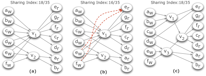
Figure 2 shows three overlays for our running example, and their sharing indexes. Figure 2(a) shows an overlay where there are multiple paths between some reader-writer pairs. As we discussed earlier, such an overlay cannot be used for a duplicate-sensitive aggregate function (like Sum, Count, etc.), but for duplicate-insensitive aggregate functions like Max, it typically leads to better sharing index as well as better overall throughput. The second overlay uses negative edges to bring down sharing index. This should only be done for aggregate functions where the subtraction operation is incrementally computable (e.g., Sum, or Count). Finally, third overlay is an example of a multi-level overlay, and has the lowest sharing index for our running example (without use of negative edges or duplicate paths). In most cases, such multi-level overlays exhibit the best sharing index. Note that multi-level overlays can also be duplicate insensitive or contain negative edges.

The problem of maximizing the sharing index is closely related to the minimum order bi-clique partition problem [23], where the goal is to cover all the edges in a bipartite graph using fewest edge-disjoint bicliques. In essence, a biclique in the bipartite graph $A_{\mathcal{G}}$ corresponds to a set of readers that all share a common set of writers. Such a biclique can thus be replaced by a partial aggregation node that aggregates the values from the common set of writers, and feeds them to the readers. In Figure 1(d), node $PA_{1}$ corresponds to such a biclique (between writers $a_{w},b_{w},c_{w}$ and readers $c_{r},d_{r},e_{r},f_{r},g_{r}$). Finding bicliques is known to be NP-Hard. Sharing index (SI) is also closely related to the compression ratio (CR) metric used in many of the works in representational graph compression  [14] ; specifically, $CR=1/(1-SI)$. However, given the context of aggregation and the possibility of having negative and duplicate-insensitive edges in the overlay, we differentiate it from compression ratio. The problem of finding a good overlay is also closely related to the problem of frequent pattern mining [30, 27] as we discuss in the next section.

3.2 Overlay Construction Algorithms

In this section, we present our algorithms for constructing different types of overlays as outlined in the previous section. Given the NP-Hardness of the basic problem, and further the requirement to scale the algorithms to graphs containing tens of millions of nodes, we develop a set of efficient heuristics to achieve our goal. Our first set of proposed algorithms (called Vnm_A, Vnm_N, and Vnm_D) builds upon a prior algorithm (called Vnm) for bipartite graph compression by Buehrer et al. [14], which itself is a adaptation of the well-known FP-Tree algorithm for frequent pattern mining [30, 27]. In our exploratory evaluation, we found that algorithm to offer the best blend of scalability and adaptability for our purposes. Our second algorithm (called Iob) is an incremental algorithm that builds the overlay one reader at a time.

3.2.1 Background: FP-Tree and VNM Algorithms

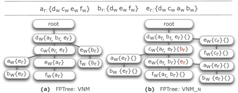
We begin with a brief recap of the FP-Tree algorithm for frequent pattern mining, considered to be one of the most efficient and scalable algorithms for finding frequent patterns. We briefly outline the algorithm using the terminology of readers and writers rather than transactions and items. First, the writers are sorted in the increasing order by their overall frequency of occurrence in the reader input sets, i.e., their out-degree in $A_{\mathcal{G}}$. In our running example, the sort order (breaking ties arbitrarily) would be $\{d_{w},c_{w},e_{w},f_{w},a_{w},b_{w}\}$. Then all the reader input lists are rewritten according to that sort order; e.g., we would write the input list of $a_{r}$ as $\{d_{w},c_{w},e_{w},f_{w}\}$. Next, the FP-Tree is built incrementally by adding one reader at a time, starting with an empty tree. For the reader under consideration, the goal is to find its longest prefix that matches with a path from the root in the FP-Tree constructed so far. As an example, Figure 3 shows the FP-Tree built after addition of readers $a_{r}$, $b_{r}$, and $e_{r}$. A node in the FP-Tree is represented by: $x_{w}\{S(x_{w})\}$ where $x_{w}$ is a writer and $S(x_{w})$ is a list of readers that contain $x_{w}$ in their input lists (called support set). Now, for reader $c_{r}$, the longest prefix of it that matches a path from root is $d_{w},c_{w},e_{w},f_{w}$. That reader would then be added to the tree nodes in that path (i.e., to the support sets along that path). If the reader input list contains any additional writers, then a new branch is created in the tree (for $e_{r}$ a new branch will be created with nodes $a_{w}\{e_{r}\}$ and $b_{w}\{e_{r}\})$.

Once the tree is built, in the mining phase, the tree is searched to find bicliques. A path $P$ in the tree from the root to the node $x_{w}\{S(x_{w})\}$ corresponds to a biclique between the writers corresponding to the nodes in $P$ and the readers in $S(x_{w})$. Since our goal is to maximize the number of edges removed from the overlay graph, we search for the biclique that maximizes:
         $benefit(P)=L(P)*|S(P)|-L(P)-|S(P)|,$
where $L(P)$ denotes the length of the path $P$ and $S(P)$ denotes the support for the last node in the path. Such a biclique can be found in time linear to the size of the FP-Tree. After finding each such biclique, ideally we should remove the corresponding edges (called the mined edges) and reconstruct the FP-Tree to find the next biclique with best benefit. Mining the same FP-Tree would still find bicliques but with lower benefit (since the next biclique we find cannot use any of the edges in the previously-output biclique).

We now briefly describe the Vnm algorithm [14], which is a highly scalable adaptation of the basic FP-Tree mining approach described above; Vnm was developed for compressing very large (web-scale) graphs, and in essence, replaces each biclique with a virtual node to reduce the total number of edges. The main optimization of Vnm relies on limiting the search space by creating small groups of readers, and looking for bicliques that only involve the readers in one of the groups. This approach is much more scalable than building an FP-Tree on the entire data graph. Vnm uses a heuristic based on shingles [18, 19] to group the readers. Shingle of a reader is effectively a signature of its input writers. If two readers have very similar adjacency lists, then with high probability, their shingle values will also be the same. In a sense, grouping readers by shingles increases the chance of finding big bicliques (with higher benefit) within the groups. The algorithm starts by computing multiple shingles for each reader, and then doing a lexicographical sort of the readers based on the shingles. The sorted list is then chunked into equal-sized groups of readers, each of which is passed to the FP-Tree algorithm separately. Mining all the reader groups once completes one iteration of the algorithm. The process is then repeated with the modified bipartite graph (where each biclique is replaced with a virtual node) to further compress the graph. Since the virtual nodes are treated as normal nodes in such subsequent iterations, a biclique containing virtual nodes may be replaced with another virtual node, resulting in connections between virtual nodes; in our context, this gives rise to multi-level overlays where partial aggregation nodes feed into other partial aggregators.

Figure 3: An example of FP-Tree construction for VNM and VNM_N: (a) Basic version, (b) FP-Tree with negative edges.

3.2.2 $VNM_{A}$: VNM Adaptive

Our first adaptation of the basic Vnm algorithm is aimed at addressing a major deficiency of that algorithm, namely lack of a systematic way to choose the chunk size. Our initial experiments with Vnm suggested that the effect of the chunk size on the final compression achieved is highly non-uniform across various graphs like web graphs and social graphs. We noticed that a bigger chunk size typically finds bigger bicliques, but it can’t find all big bicliques, especially when there is big overlap in the reader sets of two potential bicliques. This is because the reader sets of two subsequent mining phases in Vnm are mutually exclusive. Second, a bigger chunk size makes it harder to find small bicliques, which is especially a problem with later iterations; since many of the original edges have been deleted in the first few iterations, only small bicliques remain in the graph. On the other hand, using a small chunk size from the beginning ignores large bicliques that can deliver huge savings.

To address this problem, we develop an adaptive variation of Vnm that uses different chunk sizes for different iterations. For the first iteration, we use a large chunk size (100 in our experiments) and dynamically reduce it for future iterations. For the $i^{th}$ iteration, let $c_{i}$ denote the chunk size, and let $B_{i}^{s}$ denote the sum total of the benefits (defined in Section 3.2.1) for all the bicliques found in that iteration with reader set size $=s$ (note that, $s\leq c_{i}$). We choose $c_{i+1}\leq c_{i}$ to be the smallest $c$ such that: $\sum_{s\leq c}B_{i}^{s}>0.9\sum_{s\leq c_{i}}B_{i}^{s}$. Although our algorithm also requires setting two parameter values, our extensive experimental evaluation on many real-world graphs showed that the algorithm is not sensitive to the initial chunk size to within an order of magnitude, and to the second parameter between 0.8 and 1.

3.2.3 $VNM_{N}$: VNM with Negative Edges

Next, we present our adaptation to Vnm that considers adding negative edges to reduce the overlay size. In essence, we look for quasi-bicliques that may be a few edges short of being complete bicliques (this problem is also known to be NP-Hard [37]). For scalability, our algorithm employs the same basic structure as the Vnm_A algorithm discussed above (with grouping of readers using shingles); however, we modify the FP-Tree construction and mining algorithms to support negative edges.

Recall that a node in an FP-Tree is represented by $x_{w}\{S(x_{w})\}$ where $x_{w}$ is a writer and $S(x_{w})$ contains the readers that contain $x_{w}$ in their input lists. To accommodate negative edges, we now represent a node by $x_{w}\{S(x_{w})\}\{S^{\prime}(x_{w})\}$, where $S^{\prime}(x_{w})$ contains readers that do not contain $x_{w}$ in their input list, but may contain the writers corresponding to the nodes below this node in the FP-Tree. Benefit of a path $P$ in the FP-Tree is now given by:
    $benefit(P)=L(P)*|S(P)|-L(P)-|S(P)|-\sum_{P}|S^{\prime}(x_{w})|$,
where the last term captures the number of negative edges along $P$.

In our proposed algorithm, when an FP-Tree is augmented to include a new reader $r$, we add $r$ along up to $k_{1}$ paths in the FP-Tree that maximize the benefit given the FP-Tree constructed so far. More specifically, we exhaustively explore the FP-Tree in a breadth-first manner, and for each node visited, we compute the benefit of adding $r$ along the path. We then choose up to $k_{1}$ paths with the highest benefit and add the reader along those paths. As with the original FP-Tree algorithm, additional branches may have to be created for the remaining writer nodes in $r$.

Figure 3(b) shows an example where upto two paths can be added for a reader (i.e., $k_{1}=2$). Both readers $b_{r}$ and $e_{r}$ create two paths in the overlay, one of which uses a negative edge. Note that $e_{r}$ creates a new branch in the tree (apart from the one similar to in the basic version); after the introduction of negative edge for $e_{r}$ at $a_{w}$, there are still nodes remaining in $e_{r}$’s input list. During the mining phase the new FP-Tree finds a biclique of size 3x3. On the other hand, the basic version can only find a biclique of size 2x2.

Although our algorithm finds the best paths to add the reader along, it runs in time linear to the size of the FP-Tree constructed so far. However, since the FP-Tree, in essence, now encodes information about $k_{1}$ times as many readers as it did before, the size of the FP-Tree itself is expected to be larger by about the same factor. To improve efficiency, we stop the breadth-first exploration down a path if more than $k_{2}$ negative edges are needed to add $r$ along that path (we set $k_{2}=5$ in our experiments). This optimization has little impact on performance since it is unlikely that quasi-bicliques requiring a large number of negative edges will be beneficial.

3.2.4 $VNM_{D}$: Duplicate-insensitive VNM

Next, we discuss our proposed algorithm for finding overlays that exploit the duplicate-insensitive nature of some aggregates and allow for multiple paths between a writer and a reader. There are two natural ways to extend the Vnm algorithm for reusing edges in this fashion. First, we can keep the basic structure of the Vnm algorithm and modify the FP-Tree algorithm itself to find multiple bicliques in each mining phase, while ignoring the overlap between bicliques. However, by construction, the bicliques mined from a single FP-Tree tend to have very high overlap, and the benefits for additional bicliques found can be very low. It is also not clear how many aggregate nodes to add in a single mining phase; adding all bicliques for which the benefit is non-zero is likely to lead to many partial aggregate nodes, each providing low benefit.

Instead, in our proposed algorithm Vnm_D, we modify the reader grouping phase itself. In Vnm, in each iteration, the readers are grouped into disjoint groups before passing to the FP-Tree construction and mining phase. Instead, we allow the groups of readers to overlap. Specifically, given an overlap percentage $p$ (an algorithm parameter), we allow two consecutive groups of readers to have $p\%$ readers in common. The FP-Tree construction and mining phases themselves are unchanged with the following exceptions. First, instead of representing an FP-Tree node as $x_{w}\{S(x_{w})\}$, we represent it as $x_{w}\{S^{{notmined}}(x_{w})\}\{S^{{mined}}(x_{w})\}$, where $S^{{mined}}$ $(x_{w})$ contains the readers $r$ such that the edge from $x_{w}$ to $r$ was present in a previously used biclique. Second, we modify the formula for computing the benefit of a path as follows:
$benefit(P)=L(P)*|S(P)|-L(P)-|S(P)|-\sum_{P}|S^{mined}(x_{w})|$;
the last term captures the number of reused edges in the biclique.

3.2.5 IOB: Incremental Overlay Building

The overlay constructions algorithms that we have developed so far are all based on identifying sharing opportunities by looking for bicliques in $A_{\mathcal{G}}$. However, to make those algorithms scalable, two heuristics have to be used: one to partition the readers into small groups, and one to mine the bicliques themselves. In essence, both of these focus the search for sharing opportunities to small groups of readers and writers, and never consider the entire $A_{\mathcal{G}}$ at once. Next, we present an incremental algorithm for building the overlay that starts with an empty overlay, and adds one reader at a time to the overlay. For each reader, we examine the entire overlay constructed till that point which, as our experimental evaluation demonstrates, leads to more compact overlays.

We begin with ordering the readers using the shingle order as before, and add the readers one at a time in that order. In the beginning, the overlay graph simply contains the (singleton) writer nodes. Let $\langle r,\mathcal{N}(r)\rangle$ denote the next reader to be added. Let $\langle ovl_{n},\mathcal{I}(ovl_{n})\rangle$ denote a node in the overlay constructed so far, where $\mathcal{I}(ovl_{n})$ is the set of writers whose partial aggregate $ovl_{n}$ is computing. For reader $r$, our goal is to reuse as much of the partial aggregation as possible in the overlay constructed so far. In other words, we would like to find the smallest set of overlay nodes whose aggregates can be used to compute the aggregate for $r$. This problem is essentially the minimum exact set cover problem, which is known to be NP-Complete.

We use a standard greedy heuristic commonly used for solving the set cover problem. We start by finding the overlay node that has maximum overlap with $\mathcal{N}(r)$, and restructure the overlay to make use of that overlap. We keep on repeating the same process until all nodes in $\mathcal{N}(r)$ are covered (since the singleton writer nodes are also considered part of the overlay, we can always cover all the nodes in $\mathcal{N}(r)$). Let $\langle v_{1},B\rangle$ denote the overlay node that was found to have the highest overlap with the uncovered part, denoted $A$, of $\mathcal{N}(r)$. If $B\subseteq A$, then we add an edge from $v_{1}$ to $r$, and repeat the process with $A-B$. Otherwise, we restructure the overlay to add a new node $\langle v_{1}^{\prime},A\cap B\rangle$, reroute the appropriate incoming edges (i.e., the incoming edges corresponding to the writers in $A\cap B$) from $v_{1}$ to $v_{1}^{\prime}$, and add a directed edge from $v_{1}^{\prime}$ to $v_{1}$. We then also add an edge from $v_{1}^{\prime}$ to $r$. If $A-A\cap B$ is non-empty, then we repeat the process to cover the remaining inputs to $r$.

As with the Vnm-based algorithms, we use multiple iterations to improve the overlay. In each iteration (except the 1st iteration), we revisit the decisions made for each of the partial aggregator nodes, and do local restructuring of the overlay if better decisions are found for any of the partial aggregator nodes (using the same set cover-based algorithm as above).

Figure 4: An example execution of Iob algorithm for the data graph in Figure 1(a).

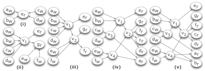
Example: Figure 4 shows an overlay built by Iob for our running example, with the readers added in order: $\{e_{r},g_{r},f_{r},c_{r},d_{r},a_{r},b_{r}\}$. Figure 4(i) shows the overlay after adding the $\langle e_{r},\{a_{w},b_{w},c_{w},d_{w}\}\rangle$. While adding the second reader, i.e., $\langle g_{r},\{a_{w},b_{w},c_{w},d_{w},e_{w},f_{w}\}\rangle$, $\mathcal{I}(e_{r})$ is found to have maximum overlap with $\mathcal{N}{(g_{r})}$. Hence, a new aggregator node $v_{1}$ (aggregating $a_{w},b_{w},c_{w},d_{w}$) is added and shared by $e_{r}$ and $g_{r}$ (Figure 4(ii)). Also direct edges are added from $e_{w}$ and $f_{w}$ to $g_{r}$ (for the inputs that were not covered). For $f_{r}$: $\mathcal{I}(g_{r})$ is found to have the maximum overlap with $\mathcal{N}(f_{r})$, leading to the construction of a new aggregator node $v_{2}$, and so on. We omit a detailed discussion of the rest of the construction due to space constraints.

For efficient execution of the algorithm we maintain both a reverse index and a forward index. For a writer node $w$, the reverse index tells us which are the overlay nodes that are aggregating $w$. For example, $a_{w}$’s reverse index entry will have both $v_{1}$ and $v_{2}$. Note that even though there is no direct edge from $a_{w}$ to $v_{2}$, $a_{w}$’s reverse index entry has $v_{2}$ because $v_{2}$ is effectively aggregating $a_{w}$. This index helps us to find the overlay node that provides maximum cover to a set of input nodes using one single scan of the input list. On the other hand, for any node $n$ in the overlay, the forward index tells us the input list of $n$. For example, $v_{2}$’s forward index entry will have $v_{1}$ and $v_{3}$ in it.

Although the above algorithm could be extended to allow for negative edges and/or duplicate paths, we do not discuss those extensions here. This is because, although Iob finds significantly smaller overlays, the overlays tend to be deep (with many levels) and in our experimental evaluation, the end-to-end throughput for the overlays was lower than for the overlays found with the Vnm_A algorithm. Thus, although the Iob algorithm is a better algorithm for finding compact overlays and for compressing bipartite graphs, Vnm-based algorithms are better suited for our purpose.

3.3 Handling Dynamic Changes

We briefly sketch our techniques to incrementally update the overlay in response to structural changes to the underlying data graph.

Addition of Edges: When a new edge is added to the data graph, we explore the neighborhoods of both the endpoints to construct a list: $\{\langle r_{1},\Delta(\mathcal{I}(r_{1}))\rangle,\langle r_{2},\Delta(\mathcal{I}(r_{2}))\rangle,...\}$, where $r_{i}$ denotes a reader whose input list has changed, and $\Delta(\mathcal{I}(r_{i}))$ denotes the new writer nodes that are added to $\mathcal{I}(r_{i})$ (for queries defined over 2-hop neighborhoods or larger, the changes to the input lists can be substantial). We process the change for each of the readers separately. If $|\Delta(\mathcal{I}(r_{i}))|$ is larger than a prespecified threshold, we use the Iob algorithm to add a new aggregate node that computes a partial aggregate over the writers in $\Delta(\mathcal{I}(r_{i}))$ (in the best case scenario, an existing overlay node may already compute exactly this aggregate); we then add an edge from that node to $r_{i}$. Otherwise, we add direct edges from the writer nodes in $\Delta(\mathcal{I}(r_{i}))$ to $r_{i}$. At the same time, for each reader in the overlay $r$, we also keep a count of direct edges from writers to that reader; this count is updated in the latter case, and if the count is larger than the threshold, we use the Iob algorithm to restructure the overlay as above.

Deletion of Edges: Edge deletions are trickier to handle because significant restructuring of the overlay may be needed, especially for multi-level overlays and complex ego-centric queries. As above, we explore the neighborhoods of the endpoints of the deleted edge to construct a list: $\{\langle r_{1},\Delta(\mathcal{I}(r_{1}))\rangle,\langle r_{2},\Delta(\mathcal{I}(r_{2}))\rangle,...\}$, and we process each reader independently. For each of the readers, we make a pre-processing pass over the overlay to identify how many of the overlay nodes would need to be modified to accommodate the change. In other words, for reader $r_{i}$, we count the number of overlay nodes $ovl$ that are upstream of $r_{i}$ and $\mathcal{I}(ovl)\cap\Delta(\mathcal{I}(r_{i}))\neq\phi$. If this number is small ($\leq 5$), we modify the overlay by splitting the overlay nodes and removing edges appropriately (we omit the details here for brevity). Otherwise, we simply remove all incoming edges to $r_{i}$ (and any partial aggregate nodes that only send values to $r_{i}$), and use the Iob algorithm to add $r_{i}$ back in with the modified input list.

Addition or Deletion of Nodes: Addition of a new node, $u$, to the data graph is easy to handle. First, we add a new writer node $u_{w}$ to the overlay, and then add direct edges from $u_{w}$ to some of the existing reader nodes as dictated by the new edges added between $u$ and the existing nodes (in most cases, a new node is added with one edge to an existing node). Second, we construct an input list for $u$, and we use the Iob algorithm to add a new reader node $u_{r}$ with that input list. On the other hand, when a node $u$ is deleted from the data graph, we simply remove $u_{w}$ and $u_{r}$ and all their incident edges from the overlay graph. We also remove $u$ from the data structures used for incremental maintenance (i.e., the forward and the reverse indexes).

Figure 5: (i) An example overlay annotated with read/write frequencies; (ii) Computing (pull, push) frequencies; (iii) Construction of the s-t augmented graph (with the annotations denoting the edge weights).

4 Making Dataflow Decisions

Next, we discuss how to make the dataflow (i.e., precomputation) decisions to maximize the total throughput given an overlay network, and the expected read/write frequencies for the nodes. Surprisingly, the problem can be solved optimally in polynomial time. We begin with the preliminaries related to the cost of a dataflow decisions and then provide the formal problem definition and present the analysis along with the algorithms that we propose.

4.1 Preliminaries

For each node $v\in V$ in the data graph, let $r(v)$ denote its read frequency (i.e., the number of times a query is issued at node $v$), let $w(v)$ denote its write frequency (i.e., the number of times $v$ is updated). Given these, with each node $u\in V^{\prime\prime}$ in the overlay graph $O_{\mathcal{G}}(V^{\prime\prime},E^{\prime\prime})$, we associate two numbers, $f_{l}(u)$ and $f_{h}(u)$, called pull frequency and push frequency, respectively. $f_{h}(u)$ captures the number of times data values would be pushed to $u$ if all nodes in the overlay are assigned push decisions. Similarly, $f_{l}(u)$ indicates the number of times data values would be pulled from $u$ if all nodes in the overlay are assigned pull decisions.

The push and pull frequencies are computed as follows. For computing push frequencies, we start by assigning $f_{h}(a_{w})=w(a_{w})$ for all writer nodes $a_{w}$, and then propagate the push frequencies from left to right (downstream). For an aggregation node or a reader node $u$, $f_{h}(u)$ is computed by summing up the push frequencies for all nodes that are immediately upstream of $u$. Similarly, the pull frequencies are computed by starting with the reader nodes, then recursively computing the pull frequencies for the rest of the nodes. Figure 5(i)-(iii) illustrates this with an example that we also use to show how our algorithm makes the dataflow decisions.

4.2 Push and Pull Costs

As discussed before, a push decision on a node implies that the aggregate corresponding to that node will be (incrementally) precomputed and will be available for immediate consumption. On the other hand, a pull decision on a node implies that the aggregate will be computed on demand when the node is read. In order to reason about the tradeoff between push and pull, we need to be able to compute the cost of a push or a pull. This cost typically depends on the nature of the aggregate, and the type and the size of the sliding window [8]. We capture these costs as two functions: $H(k)$ denotes the average cost of one push for an aggregation node with $k$ inputs, and $L(k)$ denotes the average cost of one pull for that node. For example, for a Sum aggregate node, we expect $H(k)\propto 1$ and $L(k)\propto k$, whereas for a Max aggregate node, if we use a priority queue for handling incremental updates, then $H(k)\propto\log_{2}(k)$ and $L(k)\propto k$. To handle sliding windows, we implicitly assign $w$ inputs to each writer where $w$ is the average number of values in the sliding window at a writer – thus if the sliding window is of size 10, then $PUSH$ and $PULL$ costs of the writer node will be $H(10)$ and $L(10)$ respectively. We assume $H()$ and $L()$ are either provided, or are computed through a calibration process where we invoke the aggregation function for a range of different inputs and learn the $H()$ and $L()$ functions.

4.3 Problem Definition

The dataflow decisions made by a solution induce a node partition, denoted $(X,Y),X\cap Y=\phi$, on the overlay graph, where $X$ contains nodes that are designated push, $Y$ contains nodes designated pull (Figure 5(ii)). Since all nodes upstream of a push node must also be designated push (and similarly all nodes downstream of a pull node must also be pull), the partition induced by any consistent set of dataflow decisions must satisfy the constraint that there is no edge from a node in $Y$ to a node in $X$.

For an overlay node $v$, let $PUSH(v)$ $=f_{h}(v)*H(deg(v))$ denote the cost incurred if it is designated a push node, let $PULL(v)$ $=f_{l}(v)*L(deg(v))$ denote the cost if it is a pull node. Although the push/pull decisions cannot be made for the nodes independently (because of the aforementioned constraint), $PUSH()$ and $PULL()$ costs can be computed independently; this is because the computations that happen at a node when it is invoked, do not depend on the dataflow decisions at its input or output nodes. Thus, to minimize the total computational cost, our goal reduces to finding an ($X$, $Y$) partition of the overlay (with no edges going from $Y$ to $X$) that minimizes: $\sum_{v\in X}PUSH(v)+\sum_{v\in Y}PULL(v)$.

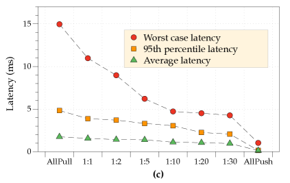
Query Latencies: Another consideration in making dataflow decision is the impact on query latencies. Throughput maximization may lead to higher use of pull decisions, especially if reads are less frequent than writes, that may result in high query latencies. As we show in Section 5, because our system is entirely in-memory and does not need to do distributed network traversals, the query latencies are quite low even in the worst-case. In future work, we plan to investigate latency-constrained optimization as well as understand the interplay between throughput and latency better.

4.4 Algorithm

We design an algorithm for a slightly more general problem that we call difference-maximizing partition problem, that we describe first.

Difference-Maximizing Partition (DMP) Problem: We are given a directed acyclic graph $H(H_{V},H_{E})$, where each vertex $v\in H_{V}$ is associated with a weight $w(v)$; $w(v)$ may be negative. For ease of exposition, we assume that $\forall v,w(v)\neq 0$. We are asked to find a graph partition $(X,Y)$, such that there are no edges from $Y$ to $X$, that maximizes: $\sum_{v\in X}w(v)-\sum_{v\in Y}w(v)$. Note that, the solution is trivially $(X=H_{V},Y=\phi)$ if all node weights are positive. We also note that, the metric has the maximum possible value if all nodes with $w(v)<0$ are assigned to $Y$, all nodes with $w(v)>0$ to $X$. However, that particular assignment may not guarantee that there are no edges from a vertex in $Y$ to a vertex in $X$.

Reducing Dataflow Decisions Problem to DMP: To reduce our problem to this problem, we set:

$w(v)=f_{l}(v)L(deg(v))-f_{h}(v)H(deg(v))$ = $PULL(v)-PUSH(v)$

That is, the weight of node $v$ is the “benefit” of assigning it a push decision (which is negative if $PULL(v)<PUSH(v)$). Then:

$$\sum_{v\in X}w(v)-\sum_{v\in Y}w(v)$$

$$=\sum_{v\in X}(PULL(V)-PUSH(v))-\sum_{v\in Y}(PULL(V)-PUSH(v))$$

$$=\underline{\sum_{v\in H_{V}}(PULL(v)+PUSH(v))}-2(\sum_{v\in X}PUSH(v)+\sum_{v\in Y}PULL(v))$$

Since the underlined term is a constant, maximizing this is equivalent to minimizing $\sum_{v\in X}PUSH(v)+\sum_{v\in Y}PULL(v)$.

Algorithm for Solving DMP: To solve this more general problem, we construct an edge-weighted graph $H^{\prime}(H^{\prime}_{V},H^{\prime}_{E})$ from $H(H_{V},H_{E})$ (in practice, we do not make a copy but rather augment $H$ in place). $H^{\prime}_{V}$ contains all the vertices in $H_{V}$ and in addition, it contains a source node $s$ and a sink node $t$ (nodes in $H^{\prime}$ are unweighted). Similarly, $H^{\prime}_{E}$ contains all the edges in $H_{E}$, with edge weights set to $\infty$. Further, for each $v\in H_{V}$ such that $w(v)<0$, we add a directed edge in $H^{\prime}$ from $s$ to $v$ with weight $w^{\prime}(s,v)=-w(v)$. Similarly for $v\in H_{V},s.t.\ w(v)>0$, we add a directed edge in $H^{\prime}$ from $v$ to $t$ with weight $w^{\prime}(v,t)=w(v)$ (see Figure 5(iii) for an example).

We note that, this construction may seem highly counter-intuitive, since a lot of nodes in $H^{\prime}$ have either no outgoing or no incoming edges and there are few, if any, directed paths from $s$ to $t$. In fact, the best case scenario for the algorithm is that: there is no directed path from $s$ to $t$. This is because, a path from $s$ to $t$ indicates a conflict between two or more nodes. The highlighted path form $s$ to $t$ in Figure 5(iii) provides an example. The best decision for node $i_{3}$ in isolation would be pull ($PULL(i_{3})=6,PUSH(i_{3})=10$), but that for $s_{r}$ is push because of its high in-degree and because $L(k)=k$ ($PULL(s_{r})=2*60=120,PUSH(s_{r})=70$). However, a pull on $i_{3}$ would force a pull on $s_{r}$, hence both of them cannot be assigned the optimal decision in isolation.

After constructing $H^{\prime}$, we find an $s$-$t$ directed min-cut in this directed graph, i.e., a set of edges $C\in H^{\prime}_{E}$ with minimum total edge-weight, such that removing those edges leaves no directed path from $s$ to $t$. Let $Y$ denote the set of nodes in $H^{\prime}$ reachable from $s$ after removing the edges in $C$ (excluding $s$), let $X$ denote the set of remaining nodes in $H^{\prime}$ (excluding $t$).

Theorem 4.1

$(X,Y)$ is a node partition of $H$ such that there are no edges from $Y$ to $X$, and $\sum_{v\in X}w(v)-\sum_{v\in Y}w(v)$ is maximized.

Proof: We prove that the original problem of finding an $(X,Y)$ partition of $H$ with the desired properties is equivalent to finding a $s$-$t$ min-cut in $H^{\prime}$.

Let $(X,Y)$ denote an optimal solution to our original problem, i.e., a partition of $H(H_{V},H_{E})$ such that the edges are directed from $X$ to $Y$ and $\sum_{v\in X}w(v)-\sum_{v\in Y}w(v)$ is maximized. Let $B=\{v\in H_{V}|w(v)<0\}$ denote the vertices that have an edge from $s$ in $H^{\prime}$, and let $A=\{v\in H_{V}|w(v)>0\}$ denote the vertices that have an edge to $t$ in $H^{\prime}$. Figure 6 shows the structure of the optimal solution, where we define $A_{1}=A\cap X,B_{1}=B\cap X,A_{2}=A\cap Y,$ and $B_{2}=B\cap Y$.

Figure 6: (i) Structure of an optimal solution, (ii) Removing C leaves no path between s and t.

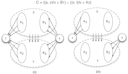
Let $C=\{(s,v)|v\in B_{1}\}\cup\{(v,t)|v\in A_{2}\}$. Since $(X,Y)$ is a partition of $H$ such that there are no (directed) edges from $Y$ to $X$, removing $C$ from $H^{\prime}$ leaves no path from $s$ to $t$ (although there are edges from $s$ to nodes in $B_{2}$ and from nodes in $A_{1}$ to $t$, there can be no path from a node in $B_{2}$ to a node in $A_{1}$ since $B_{2}\subseteq Y$ and $A_{1}\subseteq X$). In other words, $C$ is an $s$-$t$ directed cut. Now:

$$\sum_{v\in X} w(v)-\sum_{v\in Y}w(v)$$

$$=\sum_{v\in A_{1}}w(v)+\sum_{v\in B_{1}}w(v)-\sum_{v\in A_{2}}w(v)-\sum_{v\in B_{2}}w(v)$$

$$=\underline{\sum_{v\in A}w(v)-\sum_{v\in B}w(v)}-2(\sum_{v\in B_{1}}(-w(v))+\sum_{v\in A_{2}}w(v))$$

$$=\underline{\sum_{v\in A}w(v)-\sum_{v\in B}w(v)}-2(\sum_{e\in C}w^{\prime}(e))$$

Since the underlined term is a constant, the optimal solution is such that $\sum_{e\in C}w^{\prime}(e)$ is minimized, i.e., $C$ is an $s$-$t$ directed min-cut with the constraint that there is no edge from $Y$ to $X$.

Thus the last thing we need to prove is that: if $C$ is an $s$-$t$ directed min-cut of $H^{\prime}$, then the corresponding partition $(X,Y)$ of $H_{V}$ satisfies this constraint.

First we note two things. First, $C$ cannot contain any of the edges from the original edges $H_{E}$ (that all have weight $\infty$). This is because, the set of all outgoing edges from $s$ is a valid $s$-$t$ cut that has a finite value, so a min-cut must have finite value. Second, given any $s$-$t$ cut $C$ that does not include any of the original edges in $H_{E}$, we can define a corresponding partition $(X,Y)$ uniquely, where $Y$ contains nodes that are reachable from $s$ (excluding $s$), and $X$ contains the remaining nodes in $H^{\prime}_{V}$ (excluding $t$).

Assume to the contrary that, in the $(X,Y)$ partition defined by the min-cut $C$, there is a directed edge $(u,v)$ such that $u\in Y$ and $v\in X$. Since the weight of this edge is $\infty$, it will not be part of the cut. There are four cases:

• $u\in B_{2},v\in A_{1}$: Since $(s,u)$ and $(v,t)$ are $\notin C$, we get a path from $s$ to $t$, contradicting the assumption that $C$ is a cut.

• $u\in B_{2},v\in B_{1}$: This means there is a path from $s$ to $v$ (through $u$) even after deleting the edges in $C$, and thus $(s,v)$ can be removed from $C$ without compromising the property that $C$ is an $s$-$t$ cut. In other words, $C$ is not a min-cut.

• $u\in A_{2},v\in B_{1}$: Note that there must be a path from $s$ to $u$ after removing $C$, otherwise we wouldn’t need to include $(u,t)$ in the cut. Then, as above, we have a path from $s$ to $v$, and $C$ is not a min-cut.

• $u\in A_{2},v\in A_{1}$: As above, there is a path from $s$ to $u$ after removing $C$, and combined with $(v,t)$, we get a path from $s$ to $t$ contradicting the assumption that $C$ is a cut.

We thus conclude that, finding an optimal $(X,Y)$ partition of $H$ that minimizes the objective function is equivalent to finding a $s$-$t$ directed min-cut in $H^{\prime}$.

$\square$

We use the Ford-Fulkerson algorithm to construct an $s$-$t$ max-flow in $H^{\prime}$, and use it to find the optimal $(X,Y)$ partition of $H$. Specifically, after the max-flow solution has been obtained, we perform a breadth-first search from $s$ to find all nodes reachable from it in the residual graph of the max-flow, assign those nodes to $Y$, and assign the rest of the nodes to $X$.

4.5 Pre-processing

Although the above algorithm runs in polynomial time, it is not feasible to run max-flow computations on the graphs we expect to see in practice. However, a simple pre-processing pruning step, run on $H$ before augmenting it, typically results in massive reduction in the size of the graph on which the max-flow computation must be run.

Consider node $a_{w}$ in the example graph in Figure 5(ii). The best decision for that node by itself is a push decision (since $PUSH(a_{w})$ $=$ $3<PULL(a_{w})=10$). Since there is no node upstream of $a_{w}$ (which is a writer node), we can assign this node a push decision without affecting decisions at any other node (any node downstream of $a_{w}$ can still be assigned either decision), and remove it from the graph. Similarly we can assign push decision to node $b_{w}$ and remove it from $H$. After that, we can see that node $i_{1}$ can also now be assigned a push decision (optimal for it in isolation) without affecting any other node. Similarly, we can assign pull decisions to nodes $m_{r},n_{r},p_{r}$, $q_{r}$ and remove them by an analogous reasoning.

We now state the pruning rules, which are applied directly to $H$ (i.e., before constructing the augmented graph):
(P1) recursively remove all nodes $v$ such that $w(v)>0$ and $v$ has no incoming edges, and assign them push decisions,
(P2) recursively remove all nodes $v$ such that $w(v)<0$ and $v$ has no outgoing edges, and assign them pull decisions.
This pruning step can be applied in linear time over the overlay graph. We show in Section 5.3 that the graphs after pruning is much smaller than the original graph, and is usually disconnected with a large number of small connected components. We apply the above max-flow-based algorithm to each of the connected components separately.

Theorem 4.2

Use of pruning rules P1 and P2 does not compromise optimality.

Proof: Let $H$ denote the original overlay graph, and let $H^{p}$ denote the pruned graph after applying rules P1 and P2. Let $H^{\prime}$ denote the augmented graph constructed from $H$. Let $v$ denote a node that was pruned using rule P1, and thus assigned a push decision. Let $UPSTREAM(v)$ denote the set of all nodes upstream of $v$ in $H$ (including $v$). According to P1, node $v$ being pruned and assigned a push decision implies that all nodes in $UPSTREAM(v)$ must also been pruned and assigned a push decision. It follows from definition of $UPSTREAM(v)$ that there are no directed edges into $UPSTREAM(v)$ from any of the remaining nodes in $H$. Further, for any node $u\in UPSTREAM(v)$, $w(v)>0$ (for P1 to apply), and thus there is an edge $(u,t)$ in $H^{\prime}$ but no edge from $s$ to $u$. Thus, even in $H^{\prime}$, there is no edge to a node in $UPSTREAM(v)$ from one of the remaining nodes $H^{\prime}$.

Putting these together, we have that the nodes in $UPSTREAM$ $(v)$ are not reachable from $s$ in $H^{\prime}$. Thus in any network flow that originates at $s$, no flow can reach the nodes in $UPSTREAM(v)$ and those nodes do not participate in the network flow. As a result, the nodes in $UPSTREAM(v)$ will remain unreachable from $s$ in the residual graph at the end of max-flow algorithm, and hence, they will all be assigned a push decision in the end (i.e., same decision as assigned by the pruning step). By an analogous reasoning, we can show that the nodes that are pruned by the pruning rule P2 and assigned a pull decision will remain unreachable from $s$ in the residual graph of max-flow as well (this is because there is no path from those nodes to $t$, and hence they do not participate in the max-flow solution either).

Further, since the pruned nodes do not participate in the max-flow in any way, removing them does not change the max-flow solution found either. Hence, the decisions made on the pruned graph $H^{p}$ will be identical to the ones made on the original graph $H$.

$\square$

4.6 Greedy Alternative to the Max-flow-based Algorithm

Although we found the pruning step to be highly effective in reducing the complexity of the max-flow-based algorithm, we also sketch a simpler greedy algorithm for making dataflow decisions in case the pruning step results in a very large connected component (we note that we did not encounter such a scenario in our extensive experimental evaluation). We traverse the overlay graph starting from the writers in a breadth-first manner. After processing a node, it may be assigned one of three decisions: (1) push, (2) pull, (3) tentative pull. A tentative pull decision may be changed to a pull or push decision, but a pull or a push decision, once made, is final. We maintain two invariants at all times: (1) a node that is assigned a tentative pull decision is never downstream of a node assigned a pull or tentative pull decision, (2) a node assigned a push decision is never downstream of a node assigned a pull or a tentative pull decision. When processing a node $v$:

• If one of the input nodes to $v$ has been assigned a pull decision, we assign a pull decision to $v$.

• If $PUSH(v)>PULL(v)$ (i.e., the node should be assigned a pull decision) and at least one of $v$’s input nodes is assigned a tentative pull decision, then we assign a pull decision to $v$. We also change the tentative pull decisions assigned to any of its input nodes to pull.

• If $PUSH(v)>PULL(v)$ (i.e., the node should be assigned a pull decision) and none of its input nodes are assigned pull or tentative pull decisions, we assign a tentative pull decision to $v$.

• If $PUSH(v)<PULL(v)$ (i.e., the node should be assigned a push decision) and all of its input nodes are assigned a push decision: we assign a push decision to $v$.

• Finally, if $PUSH(v)<PULL(v)$ and some of its input nodes are assigned a tentative pull decision, then we make a greedy local decision for all of those nodes together. That is, we check the total cost of assigning all of those nodes a push decision and the total cost of assigning all of them a pull decision, and pick the best among the two.

It is easy to see that the algorithm maintain the two invariants at all times, and thus produces a valid set of dataflow decisions at the end (at the end, tentative pull decisions, if any, are treated as pull decisions). This greedy algorithm runs in time linear in the number of edges (each edge is processed at most twice), and is thus highly efficient.

4.7 Partial Precomputations by Splitting Nodes

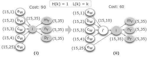
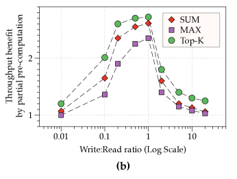
Making decisions on a per-node basis can lose out on a significant optimization opportunity – based on the push and pull frequencies, it may be beneficial to partially aggregate a subset of the inputs to an aggregate node. Figure 7 shows an example. Here, because of the low write frequencies for inputs $a_{w},b_{w},c_{w},$ and $d_{w}$ for aggregator node $i$, it is better to compute a partial aggregate over them, but compute the full aggregate (including $e_{w}$) only when needed (i.e., on a read).

One option would be to make the pre-computation decisions on a per-edge basis. However, that optimization problem is much more challenging because the cost of an incremental update for an aggregate node depends on how many of the inputs are being incrementally aggregated, and how many on demand; thus the decisions made for different edges are not independent of each other. Next we propose an algorithm that achieves the same goal, but in a much more scalable manner.

For every node $v$ in the overlay graph, we consider splitting its inputs into two groups. Let $f$ denote the pull frequency for $v$, and let $f_{1},...,f_{k}$ denote the push frequencies of its input nodes, sorted in the increasing order. For every prefix $f_{1},...,f_{l}$, of this sequence, we compute: $\sum_{i\leq l}f_{i}H(l)+f\times L(l)$. We find the value of $l$ that minimizes this cost; if $l\neq 0$ and $l\neq k$, we construct a new node $v^{\prime}$ that aggregates the inputs corresponding to frequencies $f_{1},...,f_{l}$, remove all those inputs from $v$, add $v^{\prime}$ as an input to $v$. As we show in our experimental evaluation, this optimization results in significant savings in practice.

Figure 7: Splitting a node based on push-pull frequencies.

4.8 Adapting the Dataflow Decisions

Most real-world data streams, including graph data streams, show significant variations in read/write frequencies over time. We propose and empirically evaluate, a simple adaptive scheme to handle such variations. For a subset of the overlay nodes (specified below), we monitor the observed push/pull frequencies over recent past (the window size being a system parameter). If the observed push/pull frequencies at a node are significantly different than the estimated frequencies, then we reconsider the dataflow decision just for that node and change it if deemed beneficial. Dataflow decisions can be unilaterally changed in such a manner only for: pull nodes all of whose upstream nodes are designated push, and push nodes all of whose downstream nodes are designated pull (we call this the push/pull frontier). Hence, these are the only nodes for which we monitor push/pull frequencies (it is also easier to maintain the push/pull frequencies at these nodes compared to other nodes). Techniques for more sophisticated adaptive schemes is a rich area which we plan to pursue in future.

5 Evaluation

In this section, we present a comprehensive experimental evaluation using our prototype system using several real-world information networks. Our results show that overall our approach results in significant improvements, in many cases order of magnitude improvements, in the end-to-end throughputs overall baselines, and that our overlay construction algorithms are effective at finding compact overlays.

Figure 8: Comparing overlay construction algorithms on real networks; (Iob should not be directly compared against Vnm_N or Vnm_D since it does not use negative edges or duplicate paths)

5.1 Experimental Setup

We ran our experiments on a 2.2GHz, 24-core Intel Xeon server with 64GB of memory, running 64-bit Linux. Our prototype system is implemented in Java. We use a set of dedicated threads to play back the write and read traces (i.e., to send updates and queries to the system), and a thread pool to serve the read and write queries.

Datasets and Query Workload: We evaluated our approach on several real-world information networks including :
(1) LiveJournal social network (soc-LiveJournal1: 4.8M nodes/69M edges),
(2) social circles from Google+ (ego-Gplus:107k/13M),
(3) Web graph of Berkeley and Stanford (web-BerkStan: 685k/7.6M),
(4) Hollywood-2009 Social Graph (1.1M/114M),
(5) EU2005 Web Graph (862k /19M), and
(6) UK2002 Web Graph (18.5M /298M).
In this paper, we report results for the first two, and the last two.

We report results for three ego-centric aggregate queries: Sum, Max, and Top-K, all specified over 1-hop neighborhoods. Sum and Max queries ask us to compute the total sum and the max over the input values respectively. Top-K asks for the $k$ most frequent values among the input values, and is a holistic aggregate [38].

Since the user activity patterns (i.e., read/write frequencies) are not available for any real-world network that we are aware of, we generate those synthetically using a Zipfian distribution; event rates in many applications like tweets in Twitter, page views in Yahoo!’s social platform have been shown to follow a Zipfian distribution [49, 13]. Further, we assume that the read frequency of a node is linearly related to its write frequency; we vary the write-to-read ratio itself to understand its impact on the overall performance. For some of the experiments, we used real network packet traces to simulate user activity : (1) EPA-HTTP, and (2) UCB Home IP Web Traces.

Evaluation Metric: Our main evaluation metric is the end-to-end throughput of the system, i.e., the total number of read and write queries served per second. This metric accounts for the side effects of all potentially unknown system parameters whose impact might not show up for a specifically designed metric, and thereby reveals the overall efficacy of the system. When comparing the overlay construction algorithms, we also use the following metrics: sharing index (SI), memory consumption, and running time.

Comparison Systems or Algorithms: For overlay construction, we compare five algorithms: Vnm, Vnm_A, Vnm_N, Vnm_D, and Iob. For overall throughput comparison, we compare three approaches: (1) all-pull, where all queries are evaluated on demand (i.e., no sharing of aggregates and no pre-computation), (2) all-push, where all aggregates are pre-computed, but there is no sharing of partial aggregates, and (3) dataflow-based overlay, i.e., our approach with sharing of aggregates and selective pre-computation. We chose the baselines based on industry standards: all pull is typically seen in social networks, whereas all push is more prevalent in data streams and complex event processing (CEP) systems.

5.2 Overlay Construction

Sharing Index: First we compare the overlay construction algorithms with respect to the average sharing index achieved per iteration, over 5 runs (Figure 8). As we can see, Iob finds more compact overlays (we observed this consistently for all graphs that we tried). The key reason is that: Iob considers the entire graph when looking for sharing opportunities, whereas the Vnm variations consider small groups of readers and writers based on heuristical ordering of readers and writers. Note that, Iob should only be compared against Vnm_A, and not Vnm_N or Vnm_D, since it does not use negative edges or duplicate paths. We also note that, for Iob, most of the benefit is obtained in first few iterations, whereas the VNM-based algorithms require many iterations before converging. Further, the overlays found by Vnm_N and Vnm_D are significantly better than those found by Vnm_A. This validates our hypothesis that using negative edges and reusing mined edges, if possible, results in better overlays. Another important trend that we see here is that the sharing indexes for web graphs are typically much higher those for the social graphs. Kumar et al. also notice similar difficulties in achieving good structural compression in social networks [18].

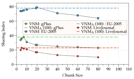
Comparing Vnm and Vnm_A: Figure 9 shows SI achieved by our adaptive Vnm_A algorithm and by Vnm_A as the chunk size is varied. As we can see, Vnm is highly sensitive to this parameter, whose optimal value is quite different for different data graphs. On the other hand, Vnm_A is able to achieve as compact an overlay (in some cases, slightly better) as the best obtained by Vnm.

Figure 9: Effect of chunk size on Vnm

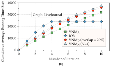
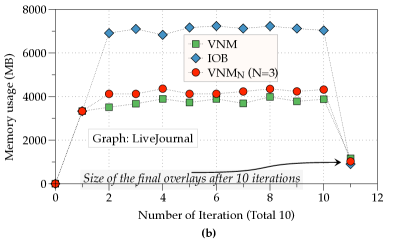
Running Time and Memory Consumption: Figure 10(a) shows the running time for the different construction algorithms with the increasing number of iterations for the LiveJournal graph. As we can see Iob takes more time for first few iterations, but is overall faster than the Vnm_A and its variations since it converges faster. As expected, both Vnm_N and Vnm_D take more time per iteration than Vnm_A. We also compared ( Figure 10(b)) the total memory consumption of the overlay construction algorithms . For LiveJournal, Vnm_A and its variations used approximated 4GB of memory, whereas Iob used 8GB at its peak; this is not surprising considering that Iob needs to maintain additional global data structures.

Figure 10: (a) Running time comparison of the overlay construction algorithms; (b) Memory consumption comparison of the overlay construction algorithms.

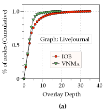
Overlay Depth: Figure 11(a) compares the depths of the overlays created by Vnm_A and Iob algorithms for one run over the LiveJournal graph. The overlay depth for a reader is defined to be the length of the longest path from one of its input writers to the reader. In the figure, we plot the cumulative distribution of the number of readers at each overlay depth. As we can see, Iob creates a significantly deeper overlay with average depth of 4.66 (vs 3.44 for Vnm_A); as we will see later, this results in lower end-to-end throughput, even though Iob creates a more compact overlay.

Figure 11: (a) Comparison of overlay depth for different overlay construction algorithms. (b) Effect of increasing parallelism on throughput.

Figure 12: (a) Benefits of pruning before running maxflow for various graphs with 1:1 write-to-read ratio; (b) Benefits of pruning before running maxflow for different write-to-read ratios on uk-2002 graph.

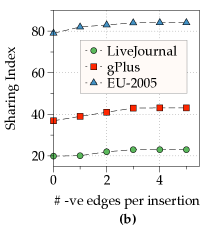
Microbenchmarking Vnm_N: Next we examine the Vnm_N algorithm and the impact of the number of negative edges allowed per transaction on the sharing index and running time. We varied the number of allowed negative edges from 1 to 5. As we can see in Figure 11(b), allowing for negative edges has a significant impact on the sharing index, and as expected, we do not see much benefit beyond 3 or 4 negative edges. The running time of Vnm_N increases rapidly as we increase the number of negative edges allowed, and almost doubles when we allow 5 negative edges vs none (not plotted). However, we note that overlay construction is a one-time process, and the benefits in terms of increased throughput outweigh the higher initial overlay construction cost.

Figure 13: (a) Effect of workload variations on different approaches; (b) Baseline to motivate dataflow decisions; (c) Read latency for different push:pull cost; (d) Effect of increasing parallelism on throughput.

Figure 14: (a) End-to-end throughput comparison for different aggregate functions for the LiveJournal graph, with 24 threads; (b) Benefits of partial pre-computation through node splitting; (c) Throughput comparison for 2-hop aggregates.

5.3 Dataflow Decisions

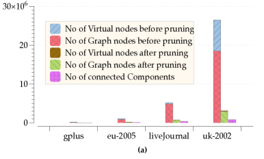
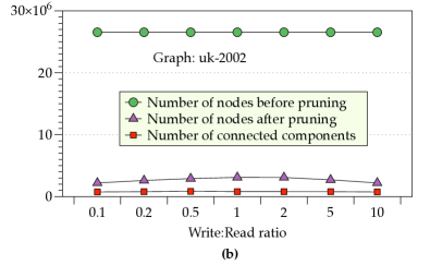
Effectiveness of Pruning: Figure 12 shows the effectiveness of our pruning strategy to reduce the input to the max-flow algorithm. In the first part, we have plotted the result for a read/write ratio of 1:1 for different data graphs. Each vertical bar in the figure has been divided to show the composition of intermediate overlay nodes and original graph nodes, before and after pruning the overlay that we got using Vnm_A. We get similar results for other overlay construction algorithms. The pruning step not only reduces the size of the graph (to below 14% in all cases), but the resulting graph is also highly disconnected with many small connected components, leading to very low running times for the max-flow computations. In Figure 12(b), we show the same results but for different write:read ratios for the uk-2002 data graph. As we can see, the benefits of pruning are lowest at write-to-read ratio of 1, which is to be expected since the possibility of conflicts is highest then. We saw similar results for the other graphs as well, demonstrating the effectiveness of pruning as well as the scalability of max-flow-based dataflow decision making under various scenarios.

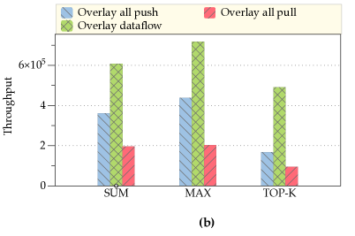
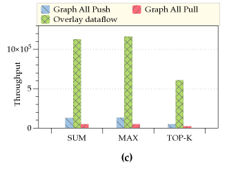
Baseline for Dataflow Decisions: Figure 13(b) shows the effectiveness of the dataflow decisions on the overlay. In this experiment we kept the number of threads (12) and read/write ratio (1:1) of the queries fixed and computed the average throughput for: (a) overlay with all push, (b) overlay with dataflow decisions, and (c) overlay with all pull. As we can see, for all aggregate functions, overlay with optimal dataflow performs much better than overlay with all pull and all push thereby justifying our hypothesis. We observed similar results for other read/write ratios as well.

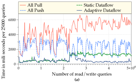
Adaptive Dataflow Decisions on a Real Trace: Figure 13(a) shows the ability of our proposed adaptive scheme to adapt to varying read/write frequencies. We used the EPA-HTTP network packet trace to simulate read/write activity for nodes. We used average read/write frequencies of the nodes to make static dataflow decisions. At a half-way point, we modified the read/write frequencies by increasing the read frequencies of a set of nodes with the highest read latencies till that point. As we can see, the static dataflow decisions turn out to be significantly suboptimal once this change is introduced. However, our simple adaptive approach is able to quickly adapt to the new set of read/write frequencies.

5.4 Throughput Comparison

Varying Read-Write Ratio: Figure 14(a) shows the results of our main end-to-end throughput comparison experiments for the three ego-centric aggregate queries. We plot the throughputs for the two baselines as well as for the overlays constructed by the different algorithms, as the write/read ratio changes from 0.05 (i.e., the workload contains mostly reads) to 20. As we can see, the overlay-based approaches consistently outperform the baselines in all scenarios. For the more realistic write/read ratios (i.e., around 1), the throughput improvement over the best of the two baselines is about a factor of 5 or 6. For read-heavy workloads, the overlay-based approach is multiple orders of magnitude better than the all-pull approach, and about a factor of 2 better than the all-push approach, whereas the reverse is true for the write-heavy workloads.

Comparing the different aggregate functions, we note that the performance improvements are much higher for the more computationally expensive Top-K aggregate function. In some sense, simple aggregates like Sum and Max represent a worst case for our approach; the total time spent in aggregate computation (which our approach aims to reduce through sharing) forms a smaller fraction of the overall running time.

Comparing the different overlay construction algorithms, we note that Vnm_N shows significant performance improvements over the rest of the overlay construction algorithms, whereas Iob is typically the worst; the higher depth of the overlay increases the total amount of work that needs to be done for both writes and reads.

Effect of Splitting Aggregate Nodes: Figure 14(b) shows the effect of our optimization of splitting an overlay aggregate node based on the push frequencies of its inputs (Section  4.5) on the LiveJournal graph. As we can see, for all the aggregate functions, this optimization increases the throughput by more than a factor of 2 when write-to-read ratio is around 1. In the two extreme cases (i.e., very low or very high write-to-read ratios) where the decisions are either all push or all pull, this optimization has less impact.

Two-hop Aggregates: Figure 14(c) shows the throughput comparison for different aggregates specified over 2-hop neighborhoods for Vnm_A overlay compared to all pull and all push; we used the write-to-read ratio of 1 over the LiveJournal graph. The relative performance of the overlay approach compared to all push or all pull is better for 2-hop aggregates than 1-hop aggregate, which can be attributed to better sharing opportunities in such queries.

Latency: Figure 13(c) shows the worst case, 95th percentile, and average latency for the read queries for Top-K as the push cost to pull cost ratio is varied. Here we used the network packet trace EPA-HTTP to simulate read/write activity. Since the number of distinct IP addresses in the trace is much smaller than the number of nodes in the (LiveJournal) graph, we randomly split the trace for each IP address among a set of nodes in the graph. We eliminated contention by ensuring that each query or update runs in isolation. As we can see, increasing the pull cost bring down the read latencies, as pushes get favored while making dataflow decision. We also note that the worst-case latencies in our system are quite low.

Parallelism: Figure 13(d) shows how the throughput varies as we increase the number of threads serving the read and write requests for the three approaches; we use the Top-K query over the LiveJournal graph, with write-to-read ratio of 1. Because of the synchronization overheads, we do not see perfect scaleup (note that the $y$-axis is in log-scale); for all three approaches, the throughput increases steadily till about 24 threads, and then plateaus out (our machine has 24 cores with hyperthreading enabled).

6 Related Work

Of the prior work on data stream management, the work on evaluating continuous aggregate queries over data streams is most closely related to our work  [7, 5, 34, 53, 9]. Arasu et al. present an SQL-based continuous query language that supports user defined aggregates and rely on mapping between streams and relations for efficient implementation [7]. Krishnamurthy et al. [34] and Wang et al. [53] present techniques for sharing work across different queries with different sliding windows. Al Moakar et al. [5] generalize that and propose a 3-level aggregation overlay. However, the sharing opportunities in ego-centric aggregate computation over graphs are fundamentally different and have not been studied in that prior work. Further, most of the prior work on evaluating continuous aggregates has only considered the all-push model of query evaluation.

There has also been much work on aggregate computation in sensor networks and distributed databases, some of which has considered sharing of partial aggregates (e.g., [51, 50, 38]). However the primary optimization goal in that work has been minimizing communication cost during distributed execution, and hence the techniques developed are quite different. There is another line of work that deals with aggregation over multiple streams mainly to support monitoring style queries [29, 46, 59]. Most of those systems either support distributed monitoring queries by aggregating over multiple streams, or provide efficient techniques to evaluate multiple aggregate queries on a single stream [34, 53, 39, 9]. Almost all of the works discussed so far either focus on static analysis of graphs or aim to do efficient distribution of data items in order to perform distributed monitoring, hence not really suitable for answering on-demand neighborhood based aggregation queries for large dynamic graphs. Several lines of work have considered the problems in deciding when to push vs pull based on monitoring read/write frequencies, in the context of replication in distributed data management systems (e.g., [55, 42]), and publish-subscribe systems (e.g., [49]). That work has typically focused on minimizing communication cost in distributed settings rather that the CPU cost of computation.

Recently, several researchers have looked at the problem of executing subgraph pattern matching queries over streaming graph data (e.g., [52]). Two extensions to SPARQL have also been proposed in recent work for specifying continuous queries over streaming RDF data [10, 6]. There is also much work on streaming algorithms for specific problems (e.g., counting triangles [32, 11], PageRank computation [20], sketching [60, 2], etc.), and on theoretical models and approximation algorithms [24, 25, 21]. However, we are not aware of any work on supporting continuous queries specified in a high-level declarative query language. Two very recent works, Kineograph [17] and GraphInc [16], also address continuous analytics over graphs. However, none of that prior work considers execution of a large number of ego-centric aggregate queries, further they do not exploit many of the optimization opportunities (e.g., aggressive sharing, pre-computations, adaptivity, etc.) that are crucial to handle very high data-rate.

Our approach to overlay construction is closely related to the prior work on compressing graphs through identifying structures such as cliques and bicliques [18, 14, 44]. As discussed in Section 3.2, the most closely related work is by Buehrer et al. [14] who propose an algorithm to find bicliques and use them to compress graphs. However, they do not consider exploiting quasi-bicliques, further, their algorithm cannot handle incremental changes to the graph. Our overlay construction algorithms can be directly applied to the bipartite graph compression problem, as we show, our algorithms produce better compression than that prior work. As a theoretical counterpart, the graph compression work by Feder and Motwani  [23] presents clique partitioning technique to compress the base graph in order to achieve better performance for some well studied graph algorithms.

Network analysis, sometimes called network science, has been a very active area of research over the last decade, with much work on network evolution and information diffusion models, community detection, centrality computation, so on. We refer the reader to well-known surveys and textbooks on that topic (see, e.g., [3, 45, 48, 12]). Increasing availability of temporally annotated network data has led many researchers to focus on designing analytical models that capture how a network evolves, with a primary focus on social networks and the Web (see, e.g., [3, 36, 35, 41]). There is also much work on understanding how communities evolve, identifying key individuals, locating hidden groups, identifying changes, visualizing the temporal evolution, in dynamic networks. Graph data mining is another well researched area where the goal is to find relevant structural patterns present in the graph  [54, 56, 30, 31]. Most of that prior work, however, focuses on off-line analysis of static datasets.

Ego-centric analysis of information networks has been getting increasing attention in recent years in network science community; here the main focus is on structural analysis of a node’s neighborhood [15, 33] as well as on answering specialized pattern matching queries [43]. In a recent work, Yan et al. [57] investigate neighborhood aggregation queries aimed at finding top-$k$ nodes (w.r.t. their aggregate values over their $h$-hop neighborhood) in the entire graph. They develop pruning techniques by noting that the aggregate values of two adjacent nodes are similar. However, they focus on static graphs and they do not consider continuous evaluation of a large number of ego-centric queries simultaneously.

7 Conclusions

In this paper, we presented the design of a continuous query processing system to efficiently process large numbers of ego-centric aggregation queries over highly dynamic, large-scale graphs. Our definition of an ego-centric aggregation query is very general, and captures a range of querying and analytics tasks including personalized trend detection, anomaly or event detection, and even complex real-time analytics over neighborhoods in the graph. We proposed a general framework that supports user-defined aggregate queries and enables efficient evaluation of such queries over highly dynamic graphs; we also developed novel scalable algorithms for exploiting sharing opportunities and for making dataflow decisions based on expected activity patterns. Our system is able to handle graphs containing 320M nodes and edges on a single machine with 64GB of memory, achieving update and query throughputs over 500k/s. With the large-memory, many-core machines that are available today, we expect such a centralized approach to be sufficient in most application domains. However, our approach is also naturally parallelizable through use of standard graph partitioning-based techniques. The readers can be partitioned in a disjoint fashion over a set of machines, and for each machine, an overlay can be constructed for the readers assigned to that machine; the writes for each writer would be sent to all the machines where they are needed.

Acknowledgments: This work was supported by NSF under grant IIS-1319432, by Air Force Research Lab (AFRL) under contract FA8750-10-C-0191 and by an IBM Faculty Award.

References

- [1] F. Abel, Q. Gao, G.-J. Houben, and K. Tao. Analyzing user modeling on twitter for personalized news recommendations. In User Modeling, Adaption and Personalization. Springer, 2011.
- [2] C. C. Aggarwal, Y. Li, P. S. Yu, and R. Jin. On dense pattern mining in graph streams. Proc. VLDB Endow., 3(1-2), 2010.
- [3] C. C. Aggarwal and H. Wang, editors. Managing and mining graph data. Springer, 2010.
- [4] L. Akoglu, M. McGlohon, and C. Faloutsos. Oddball: Spotting anomalies in weighted graphs. In KDD. Springer, 2010.
- [5] L. Al Moakar. Class-Based Continuous Query Scheduling in Data Stream Management Systems. PhD thesis, Univ. of Pittsburgh, 2013.
- [6] D. Anicic, P. Fodor, S. Rudolph, and N. Stojanovic. EP-SPARQL: a unified language for event processing and stream reasoning. In WWW, 2011.
- [7] A. Arasu, S. Babu, and J. Widom. The CQL continuous query language: semantic foundations and query execution. VLDB, 2006.
- [8] A. Arasu and J. Widom. Resource sharing in continuous sliding-window aggregates. In VLDB, 2004.
- [9] B. Babcock, M. Datar, and R. Motwani. Load Shedding for Aggregation Queries over Data Streams. In ICDE, 2004.
- [10] D. F. Barbieri, D. Braga, S. Ceri, and M. Grossniklaus. An execution environment for C-SPARQL queries. In EDBT, 2010.
- [11] L. Becchetti, P. Boldi, C. Castillo, and A. Gionis. Efficient semi-streaming algorithms for local triangle counting in massive graphs. In Proceedings of the 14th ACM SIGKDD international conference on Knowledge discovery and data mining, pages 16–24, 2008.
- [12] S. Boccaletti, V. Latora, Y. Moreno, M. Chavez, and D.-U. Hwang. Complex networks: Structure and dynamics. Physics reports, 2006.
- [13] L. Breslau, P. Cao, L. Fan, G. Phillips, and S. Shenker. Web caching and Zipf-like distributions: Evidence and implications. In INFOCOM, 1999.
- [14] G. Buehrer and K. Chellapilla. A scalable pattern mining approach to web graph compression with communities. In WSDM, 2008.
- [15] R. S. Burt. Structural holes: the social structure of competition. Harvard University Press, 1992.
- [16] Z. Cai, D. Logothetis, and G. Siganos. Facilitating real-time graph mining. In CloudDB, 2012.
- [17] R. Cheng, J. Hong, A. Kyrola, Y. Miao, X. Weng, M. Wu, F. Yang, L. Zhou, F. Zhao, and E. Chen. Kineograph: taking the pulse of a fast-changing and connected world. In EUROSYS, 2012.
- [18] F. Chierichetti, R. Kumar, S. Lattanzi, M. Mitzenmacher, A. Panconesi, and P. Raghavan. On compressing social networks. In SIGKDD, 2009.
- [19] E. Cohen, M. Datar, S. Fujiwara, A. Gionis, P. Indyk, R. Motwani, J. D. Ullman, and C. Yang. Finding Interesting Associations without Support Pruning. In ICDE, 2000.
- [20] A. Das Sarma, S. Gollapudi, and R. Panigrahy. Estimating pagerank on graph streams. In Proceedings of the twenty-seventh ACM SIGMOD-SIGACT-SIGART symposium on Principles of database systems, PODS ’08, pages 69–78, 2008.
- [21] C. Demetrescu, I. Finocchi, and A. Ribichini. Trading off space for passes in graph streaming problems. ACM Trans. Algorithms, 6:6:1–6:17, December 2009.
- [22] M. Everett and S. Borgatti. Ego network betweenness. Social networks, 2005.
- [23] T. Feder and R. Motwani. Clique partitions, graph compression and speeding-up algorithms. In STOC, 1991.
- [24] J. Feigenbaum, S. Kannan, A. McGregor, S. Suri, and J. Zhang. On graph problems in a semi-streaming model. In In proceedings of the ICALP Conference, pages 17–44, 2004.
- [25] J. Feigenbaum, S. Kannan, A. McGregor, S. Suri, and J. Zhang. Graph distances in the streaming model: the value of space. In Proceedings of the sixteenth annual ACM-SIAM symposium on Discrete algorithms, pages 745–754, 2005.
- [26] I. Guy, N. Zwerdling, I. Ronen, D. Carmel, and E. Uziel. Social media recommendation based on people and tags. In SIGIR, 2010.
- [27] J. Han, J. Pei, and Y. Yin. Mining frequent patterns without candidate generation. In SIGMOD, 2000.
- [28] J. M. Hellerstein, C. Ré, F. Schoppmann, D. Z. Wang, E. Fratkin, A. Gorajek, K. S. Ng, C. Welton, X. Feng, K. Li, et al. The MADlib analytics library: or MAD skills, the SQL. VLDB, 2012.
- [29] R. Huebsch, M. N. Garofalakis, J. M. Hellerstein, and I. Stoica. Sharing aggregate computation for distributed queries. In SIGMOD, 2007.
- [30] A. Inokuchi, T. Washio, and H. Motoda. An Apriori-Based Algorithm for Mining Frequent Substructures from Graph Data. In PKDD, 2000.
- [31] A. Inokuchi, T. Washio, and H. Motoda. Complete Mining of Frequent Patterns from Graphs: Mining Graph Data. JMLR, 2003.
- [32] H. Jowhari and M. Ghodsi. New streaming algorithms for counting triangles in graphs. In L. Wang, editor, Computing and Combinatorics, volume 3595 of Lecture Notes in Computer Science, pages 710–716. Springer Berlin / Heidelberg, 2005.
- [33] J. M. Kleinberg, S. Suri, E. Tardos, and T. Wexler. Strategic network formation with structural holes. SIGecom, 2008.
- [34] S. Krishnamurthy, C. Wu, and M. J. Franklin. On-the-fly sharing for streamed aggregation. In SIGMOD, 2006.
- [35] R. Kumar, J. Novak, and A. Tomkins. Structure and evolution of online social networks. In Link Mining: Models, Algorithms, and Applications. Springer, 2010.
- [36] J. Leskovec, L. Backstrom, R. Kumar, and A. Tomkins. Microscopic evolution of social networks. In SIGKDD, 2008.
- [37] X. Liu, J. Li, and L. Wang. Quasi-bicliques: Complexity and binding pairs. In Computing and Combinatorics. Springer, 2008.
- [38] S. Madden, M. J. Franklin, J. M. Hellerstein, and W. Hong. TAG: a Tiny Aggregation service for Ad-Hoc sensor networks. In OSDI, 2002.
- [39] S. Madden, R. Szewczyk, M. J. Franklin, and D. E. Culler. Supporting Aggregate Queries Over Ad-Hoc Wireless Sensor Networks. In WMSCA, 2002.
- [40] J. J. McAuley and J. Leskovec. Learning to discover social circles in ego networks. In NIPS, 2012.
- [41] A. Mislove, M. Marcon, K. P. Gummadi, P. Druschel, and B. Bhattacharjee. Measurement and analysis of online social networks. In SIGCOMM, 2007.
- [42] J. Mondal and A. Deshpande. Managing large dynamic graphs efficiently. In SIGMOD, 2012.
- [43] W. E. Moustafa, A. Deshpande, and L. Getoor. Ego-centric graph pattern census. In ICDE, 2012.
- [44] S. Navlakha, R. Rastogi, and N. Shrivastava. Graph summarization with bounded error. In SIGMOD, 2008.
- [45] M. E. Newman. The structure and function of complex networks. SIAM review, 2003.
- [46] C. Olston, J. Jiang, and J. Widom. Adaptive filters for continuous queries over distributed data streams. In SIGMOD, 2003.
- [47] B. A. Prakash, N. Valler, D. Andersen, M. Faloutsos, and C. Faloutsos. Bgp-lens: Patterns and anomalies in internet routing updates. In SIGKDD, 2009.
- [48] J. Scott and P. J. Carrington. The SAGE handbook of social network analysis. SAGE publications, 2011.
- [49] A. Silberstein, J. Terrace, B. F. Cooper, and R. Ramakrishnan. Feeding frenzy: selectively materializing users’ event feeds. In SIGMOD, 2010.
- [50] A. Silberstein and J. Yang. Many-to-Many Aggregation for Sensor Networks. In ICDE, 2007.
- [51] N. Trigoni, Y. Yao, A. J. Demers, J. Gehrke, and R. Rajaraman. Multi-query Optimization for Sensor Networks. In DCOSS, 2005.
- [52] C. Wang and L. Chen. Continuous subgraph pattern search over graph streams. In ICDE, 2009.
- [53] S. Wang, E. A. Rundensteiner, S. Ganguly, and S. Bhatnagar. State-Slice: New Paradigm of Multi-query Optimization of Window-based Stream Queries. In VLDB, 2006.
- [54] T. Washio and H. Motoda. State of the art of graph-based data mining. SIGKDD, 2003.
- [55] O. Wolfson, S. Jajodia, and Y. Huang. An adaptive data replication algorithm. TODS, 1997.
- [56] X. Yan and J. Han. gSpan: Graph-Based Substructure Pattern Mining. In ICDE, 2002.
- [57] X. Yan, B. He, F. Zhu, and J. Han. Top-K aggregation queries over large networks. In ICDE, 2010.
- [58] Y. Yu, P. K. Gunda, and M. Isard. Distributed aggregation for data-pa- rallel computing: interfaces and implementations. In SIGOPS, 2009.
- [59] R. Zhang, N. Koudas, B. C. Ooi, and D. Srivastava. Multiple aggregations over data streams. In SIGMOD, 2005.
- [60] P. Zhao, C. C. Aggarwal, and M. Wang. gsketch: on query estimation in graph streams. Proc. VLDB Endow., 5(3), 2011.