Pricing and clearing combinatorial markets with singleton and swap orders

Abstract

In this article we consider combinatorial markets with valuations only for singletons and pairs of buy/sell-orders for swapping two items in equal quantity. We provide an algorithm that permits polynomial time market-clearing and -pricing. The results are presented in the context of our main application: the futures opening auction problem. Futures contracts are an important tool to mitigate market risk and counterparty credit risk. In futures markets these contracts can be traded with varying expiration dates and underlyings. A common hedging strategy is to roll positions forward into the next expiration date, however this strategy comes with significant operational risk. To address this risk, exchanges started to offer so-called futures contract combinations, which allow the traders for swapping two futures contracts with different expiration dates or for swapping two futures contracts with different underlyings. In theory, the price is in both cases the difference of the two involved futures contracts. However, in particular in the opening auctions price inefficiencies often occur due to suboptimal clearing, leading to potential arbitrage opportunities. We present a minimum cost flow formulation of the futures opening auction problem that guarantees consistent prices. The core ideas are to model orders as arcs in a network, to enforce the equilibrium conditions with the help of two hierarchical objectives, and to combine these objectives into a single weighted objective while preserving the price information of dual optimal solutions. The resulting optimization problem can be solved in polynomial time and computational tests establish an empirical performance suitable for production environments.

Introduction

Futures contracts are some of the most liquid derivatives and, among other purposes, are an integral component of many hedging and risk mitigation strategies. For example, airlines regularly use futures to hedge against volatile crude prices and lock-in the current price level. These hedging strategies usually involve a rollover of the contracts from one expiration date (also called maturity) into the next when approaching the expiration date of the first. However, rolling the contracts forwards is not without risk, the so-called rollover risk. This risk consists of basically two components. The first component is the time spread risk (also called calendar spread risk), which is affected by whether the price difference between the maturing contract and the replacement contract with the extended expiration date matches the theoretical fair value. The other component, the slippage, is of an operational risk type. It is the risk of loss arising from selling off the old contracts and buying the new contracts being not perfectly simultaneous allowing for adversarial intermediate price moves or in an opening auction only one of the two orders being executed; we refer the interested reader e.g., to (Hull, 2006; Cooper, 2015) for a discussion. While the time spread risk is market inherent and hence exchange unspecific, slippage can be mitigated by the exchange by offering futures swap products, so-called combinations and various futures exchanges, such as e.g., http://www.eurexchange.comEUREX (European Exchange AG) offer such products. However, offering such products improves market transparency and liquidity only if those products are consistently priced and while this is ensured by arbitrageurs intraday, this is not necessarily the case for the opening auction when the market opens. In fact, it has been observed that in the opening auctions in some cases prices across products are inconsistent, creating potential arbitrage opportunities.

We present an efficient optimization model that guarantees consistent prices at the end of the opening auction while maximizing economic surplus. We further demonstrate that the model can be solved extremely fast in practice for large amounts of orders and contract types making it a prime candidate for production environments. The presented model is motivated by the product offering of EUREX, however it applies readily to various other futures exchanges.

Related work

The futures opening auction is a combinatorial auction and there exists a large body of work studying this type of auctions; we refer the interested reader to the very nice surveys of de Vries and Vohra (2003) and Blumrosen and Nisan (2007) for an introduction. It is well-known that various combinatorial auctions can be solved in polynomial time provided, e.g., if the constraint matrix is totally unimodular and the right-hand side of the clearing program is integral. As we will see later, our setup admits such an efficient formulation via a network flow formulation.

Closely related to our work is the work of Winter et al (2011), which is based on the master’s thesis of M. Rudel. The authors developed a pure linear integer program to solve the problem for at most three futures contract types. The approach heavily relies on preprocessing techniques to reduce the problem size for the three contracts case and while the underlying formulation is based on a network flow problem with orders modeled as arcs this structure is not exploited. In fact, the employed model is heavily driven by price conditions that involve binary variables. These binary variables render the underlying structure inaccessible and the properties of equilibrium conditions cannot be exploited. Our approach is highly superior as we naturally observe market equilibria conditions from the dual linear program as well as ensure volume maximization by appropriate objective function regularization. We provide a comparison of both approaches in Section 5.2.

There is also a significant amount of literature on so-called linear prices, which are also referred to as uniform prices. In the absence of integer variables the dual variables of the clearing conditions provide us with linear prices if we maximize the economic surplus. In previous work (Martin, Müller, and Pokutta, 2014) we used this property to ensure the existence of linear prices in European day-ahead electricity auctions. In this work, however, we exploit this property in order to get a computationally advantageous model formulation.

Contribution

We provide a natural formulation for the real-world problem of clearing, pricing, and maximizing the execution volume of a certain combinatorial exchange. We show that one can compute a solution to that problem by solving a single min cost flow problem. More precisely, we decompose the problem into a primal min cost flow problem with a weighted objective and a dual pricing problem that is closely related to the primal one. An optimal extreme point of the weighted problem is a welfare maximizing and volume maximizing clearing solution. Moreover we show that we can scale and round a dual optimal extreme point of the weighted problem to obtain the corresponding competitive equilibrium prices. In other words, the weighted problem is chosen in such a way that a primal optimal extreme point maximizes the executed volume while the desired equilibrium conditions are satisfied automatically: completely satisfied participants, positive bid-ask spreads, uncrossed order books, and the absence of combinatorial matching cycles.

This new formulation has three major advantages. First, the model is solvable in polynomial time with a standard solver and the numerical results indicate that the computing times are sufficiently fast for the use in production environments. In particular, the algorithm is significantly faster (two orders of magnitude) than the approach presented in Winter et al (2011). Second, the model is very flexible: in contrast to previous models it is not restricted to a limited number of different underlyings (e.g., one) or expiration dates (e.g., three). It is capable to handle all kinds of singleton and swap orders simultaneously, regardless of their underlyings or expirations dates. In particular, it can handle so-called time spread combinations and inter-product spread combinations in one single auction (see Def. 3). Third, the obtained prices are of high quality, that is, the prices for contracts are consistent with the prices for combinations.

Another important advantage of our integrated model is that the total economic surplus of all participants is maximized, i.e., it is not possible to find a solution with a higher economic surplus. In particular, our algorithm is superior to the current algorithm at EUREX which does not guarantee maximum economic surplus. In fact, the currently employed algorithm first determines prices for each contract separately, without taking combination orders into account. At that time the prices can therefore be inconsistent with respect to the crossed order books of combination orders. Nevertheless, the combination orders get triggered according to the prices of the underlying contracts and thus the market is not necessarily in a maximized surplus situation.

Electronic futures exchanges

Futures contracts are standardized financial products that are traded at futures exchanges. These exchanges provide electronic interfaces such that any trader around the world can advise his or her broker to route a buy or sell order directly to a futures exchange. The exchange collects those orders and stores them in order books [see Gould et al (2013) for a survey on limit order books]. There is one order book for each financial product. During the trading-hours (intraday), the exchange will execute all incoming orders that can be matched and immediately determine and publish the market clearing price at which these orders where executed. However, at the beginning of the trading day, the order books are not empty. On the one hand, there are the non-executed orders of the previous day, on the other hand, some participants already submit their orders before the trading day has started. For that reason, the exchange performs a so-called opening auction immediately before the trading day begins. In practice, the exchange determines a separate market clearing price for each financial product and only matches orders within an order book; dependencies between books are ignored. Our new approach performs a single computation that takes all order books into account and correctly models the relationships between all financial products.

The available financial products are futures contracts as well as futures contract combinations. We briefly recall the formal definition of these financial products. More detailed information on futures can be found in Chapter 2 in Hull (2006).

Definition 1

A futures contract is an agreement between two parties to

1. Buy or sell an asset (the underlying)

2. At an agreed-upon time in the future (the expiration date)

3. For an agreed-upon price (the current market clearing price of the futures contract, also called futures price).

Each (underlying, expiration date)-tuple is a financial product of the futures contract type, in particular it is an exchange tradable good with its own order book. In the following, for brevity we will also refer to futures contracts simply as contracts.

Example 1

On January 4 a trader in Frankfurt wants to buy 100 troy ounces gold with delivery in June of the same year. A single gold futures contract at EUREX has the value of 100 troy ounces. The trading day starts at 8:00 in the morning. At 7:30, he submits a buy order via his online broker to the futures exchange. The order contains the information that he wants to buy one gold futures contract, with delivery in June and that he is willing to pay at most $1069.40\text{\,}\mathrm{U}\mathrm{S}\mathrm{D}$. On the same day, another trader in Darmstadt wants to sell a gold futures contract with delivery in June of the same year. At 7:45 she submits her sell order via her online broker to the exchange. The lowest price she is willing to accept amounts to $1069.20\text{\,}\mathrm{U}\mathrm{S}\mathrm{D}$. At the opening auction at 8:00 the order book only contains these two orders. The exchange executes both orders at the market clearing price of $1069.30\text{\,}\mathrm{U}\mathrm{S}\mathrm{D}$ and publishes that price.

The previous example illustrates that during an auction two contracts are equal if the underlying and the expiration date coincide. As long as the auction is not terminated the contracts are not yet binding and the final price is not yet agreed-upon. In the moment when the auction terminates the contracts of the executed orders become binding and the agreed-upon price for the underlying at the expiration date is the market clearing price that was determined by the exchange.

Beside plain futures contracts, the participants can also trade contract combinations:

Definition 2

A futures contract combination (short: combination) allows for swapping one futures contract for another futures contract.

There are two different kinds of futures contract combinations:

Definition 3

A time spread combination allows for swapping two futures contracts with the same underlying but with different expiration dates. An inter-product spread combination allows for swapping two futures contracts with different underlyings but not necessarily different expiration dates.

Each 2-element set of (underlying, expiration date)-tuples is a financial product of the contract combination type, in particular it is an exchange tradable good with its own order book. It is a question of definition, which contract will be bought and which one will be sold if someone buys (or sells) a combination.

Our opening auction model follows the one that is currently employed by EUREX and many other exchanges follow a similar setup, so that our setup can be readily applied. In the opening auction there are two different order types: limit orders and market orders. If a participant submits a http://www.sec.gov/answers/limit.htmlimit order, then the exchange receives the following information: the ID of the financial product, whether it should be bought or sold, the maximum quantity to be bought or sold, and the limit price. The limit price specifies the highest price per unit a buyer is willing to pay or the lowest price per unit a seller is willing to accept. If a participant submits a http://www.sec.gov/answers/mktord.htmmarket order, the exchange only receives the ID of the financial product, whether it should be bought or sold, and the maximum quantity. Market orders have a higher priority than limit orders and the trader is accepting all prices. In an opening auction a market order can be treated as a limit order with the highest feasible limit price (defined by the exchange) if it is a buy order, or the lowest feasible limit price if it is a sell order; therefore, we do not need to model them explicitly and in the following all orders are of limit type.

A partial execution of limit orders or market orders is only feasible if the limit price coincides with the market clearing price. Fractional partial executions are infeasible, as contracts are indivisible; therefore, a partial execution must trade an integral number of contracts. For the sake of completeness, we want to mention that the fill-or-kill order type, which must either be executed entirely or not executed at all, is not available in the opening auction.

Modeling orders as directed arcs

In the opening auction, the participants express their preferences by submitting limit orders to the exchange. In order to model these limit orders we define several sets, input parameters, and variables.

Let $T$ be the set of the different contracts the participants can bid for. Hereinafter $T$ is also referred to as the contract set. Remember that a contract is characterized by its underlying asset and its expiration date. Two contracts are equal if they have the same underlying asset and the same expiration date. Let the contract set be a totally ordered set sorted in ascending order, where the first sort criterion is the underlying asset ID and the second criterion is the expiration date.

The main idea of the model is to treat the contracts as nodes in a graph and the orders as directed arcs connecting the nodes. To be able to model all orders as arcs, we introduce a super node $\circ$ that represents the source or sink of orders that only involve a single futures contract. The super node can be interpreted as cash. Let $T^{\prime}=T\cup\{\circ\}$ be the extended node set (contract set) so that $\circ$ becomes the new maximum. Then all orders can be modeled as arcs in $T^{\prime}\times T^{\prime}$.

Definition 4

A directed arc $(r,s)\in T^{\prime}\times T^{\prime}$ models an order for demanding $r$ and offering $s$. The case $r=s$ is not allowed. The arc represents a buy order if $r<s$. Otherwise, it represents a sell order. Per definition $r<\circ$ for all $r\in T$.

Examples for contracts $r\neq s\in T$:

Arc Buy/Sell Product Meaning

$$(r,\circ) \text{contract }r \text{demand contract }r$$ buy

$$(\circ,s) \text{contract }s \text{offer contract }s$$ sell

$$(r,s)\text{ with }r<s \text{combination }\{r,s\} r s$$ buy demand contract and offer contract

$$(s,r)\text{ with }r<s \text{combination }\{r,s\} \text{demand contract $s$ and offer contract $r$}.$$ sell

Note that the arcs $(r,s)$ and $(s,r)$ refer to the same financial product: the futures contract combination $\{r,s\}$.

Remark 1

The super node $\circ$ is only used to visualize orders in a graph. We will omit it in the LP representation of the network flow model, as the flow conservation equation of the super node is a redundant equation and is a source of degeneracy in the dual LP.

The set of limit orders (and market orders) is denoted by $I$ and hereinafter also referred to as the order book. To model an order ${i\in I}$ we use the parameters $\overline{\delta}_{i}$, $p_{i,t}$, and $Q_{i,t}$ with $t\in T$. The first parameter $\overline{\delta}_{i}\in\mathbb{N}_{+}$ models the demanded/offered quantity. The second parameter $p_{i,t}$ is the $t$-th entry of a price vector $p_{i}\in\mathbb{Z}^{T}$ that represents the limit price of order $i$. And $Q_{i,t}$ is the $t$-th entry of the characteristic vector $Q_{i}\in\{-1,0,1\}^{T}$ of the arc associated with order $i$. If $(r,s)$ is the arc associated with $i$ and $t=\min\{r,s\}$ is the smallest index, then the price vector $p_{i}$ vanishes at the entries $T\setminus\{t\}$ and the entry $p_{i,t}$ is the limit price of order $i$. The execution state of order $i$ is represented by a non-negative integer variable $\delta_{i}$.

In other words, let $(r,s)$ be the arc associated with order ${i\in I}$, then the input parameters are filled as follows: for all $t\in T$

$$Q_{i,t} \in\{-1,0,1\} Q_{i,t}=\begin{cases}+1&\text{ if }t=r\text{ (demand contract $r$)}\\ -1&\text{ if }t=s\text{ (offer contract $s$)}\\ 0&\text{ otherwise}\end{cases}$$

$$p_{i,t} \in\mathbb{Z} p_{i,t}=\begin{cases}\text{limit price of order $i$}&\text{ if }t=\min\{r,s\}\\ 0&\text{ otherwise}\end{cases}$$

$$\overline{\delta}_{i} \in\mathbb{N}_{+} \overline{\delta}_{i}=\text{ maximal demanded/offered quantity of order $i$}.$$

And the solution variables are interpreted as follows:

$$\delta_{i} \in[0,\overline{\delta}_{i}]\cap\mathbb{Z} \delta_{i}=\begin{cases}\overline{\delta}_{i}&\text{$i$\ is completely executed}\\ \text{otherwise}&\text{$i$\ is partially executed}\\ 0&\text{$i$\ is not executed}\end{cases}$$

$$\pi_{t} \in\mathbb{Z} \pi_{t}=\text{market clearing price per unit for contract {$t\in T$}}.$$

Note that the market clearing price for combinations is given by the difference of the prices of the two underlying contracts: The price of combination $\{r,s\}$ with $r<s$ is given by $\pi_{r}-\pi_{s}$. Therefore, it is not necessary to model them explicitly. The market clearing prices determine the amount of money a participant has to pay or receive for the execution of his or her order. For an order $i$ the net amount of money to be paid or received is given by

$$\sum_{t\in T}\pi_{t}Q_{i,t}\delta_{i}.$$ (1)

If this amount is positive one has to pay money, otherwise one will receive money. Similarly, we can determine the net amount a participant is willing to pay for the execution of his or her order:

$$\sum_{t\in T}p_{i,t}Q_{i,t}\delta_{i}.$$ (2)

If this amount is negative the participant wants to receive money for the execution of his or her order. The difference of the two terms is the surplus:

$$\sum_{t\in T}p_{i,t}Q_{i,t}\delta_{i}-\sum_{t\in T}\pi_{t}Q_{i,t}\delta_{i}.$$ (3)

The participant incurs a loss if this term is negative.

Example 2

Assume that there are three different contracts $T=\{1,2,3\}$. An order ${i\in I}$ for buying contract $1$ with limit price $40$ is represented by the arc $(1,\circ)$ and modeled as follows:

$$Q_{i}=\begin{pmatrix}1&0&0\end{pmatrix}^{\top}\qquad p_{i}=\begin{pmatrix}40&0&0\end{pmatrix}^{\top}.$$

And an order $j\in I$ for selling contract $2$ with limit price $53$ is represented by the arc $(\circ,2)$ and modeled by

$$Q_{j}=\begin{pmatrix}0&-1&0\end{pmatrix}^{\top}\qquad p_{j}=\begin{pmatrix}0&53&0\end{pmatrix}^{\top}.$$

Whereas an order $k\in I$ for buying contract $1$ and selling contract $2$ with a minimal spread (the limit price) of at least $13$ currency units is represented by the arc $(1,2)$ and modeled by directly involving the minimal spread:

$$Q_{k}=\begin{pmatrix}1&-1&0\end{pmatrix}^{\top}\qquad p_{k}=\begin{pmatrix}-13&0&0\end{pmatrix}^{\top}.$$

Alternatively we can also use reference prices for the two underlying contracts:

$$Q_{k}=\begin{pmatrix}1&-1&0\end{pmatrix}^{\top}\qquad p_{k}=\begin{pmatrix}40&53&0\end{pmatrix}^{\top}.$$

The negative limit price indicates that the buyer wants to receive at least 13 currency units. In practice, we use the first encoding since it only involves one price: the limit price of the combination order.

Observe that if we model a single buy or sell order, then the quantity vector and the price vector vanish at all but one entry. If we model a combination order, being a linear combination of a single buy and a single sell order, then the quantity vector vanishes at all but two entries. As order $k$ is a linear combination of order $i$ and $j$, we can write $Q_{i}+Q_{j}=Q_{k}$ and $p_{i}+p_{j}=p_{k}$.

Derivation of an hierarchical min cost flow model to be solved by the exchange

In the opening auction, the exchange determines the orders that will be executed and the prices at which those orders are executed. The employed algorithm that performs this task implements the market rules of the exchange. These rules include quantity constraints as well as price constraints. We propose an algorithm which solves an optimization problem that couples interdependent market products, guarantees consistent prices, and covers all given market rules. The objective is to maximize the executed volume subject to the quantity and price constraints:

$$\max\quad \sum_{i\in I}\delta_{i}$$ (MIP)

$$\mathop{\rm s.t.}\quad \forall{t\in T} \sum_{i\in I}Q_{i,t}\delta_{i}=0$$ clearing constraint (4)

$$\forall{i\in I} \delta_{i}>0\quad\Rightarrow\quad\sum_{t\in T}(p_{i,t}-\pi_{t})Q_{i,t}\geq 0$$ price condition (5)

$$\forall{i\in I} \delta_{i}<\overline{\delta}_{i}\quad\Rightarrow\quad\sum_{t\in T}(p_{i,t}-\pi_{t})Q_{i,t}\leq 0$$ price condition (6)

$$\forall{i\in I} 0\leq\delta_{i}\leq\overline{\delta}_{i}$$ quantity restriction (7)

$$\forall{i\in I} \delta_{i}\in\mathbb{Z}$$ integrality constraint (8)

$$\forall{t\in T} \pi_{t}\in\mathbb{Z}$$ price variable (9)

The price conditions (5) and (6) are so-called indicator constraints, which can be modeled with linear constraints by using big-M formulations. The first price constraint ensures that no participant incurs a loss if his or her order is executed. If, for example, the order is an executed buy order, then the products market price must be smaller than or equal to the limit price of the order. The second price constraint ensures that if a buy order (sell order) is not executed entirely, then the products market price must be greater than (smaller than) or equal to the limit price. Later we will see that both price conditions together actually ensure that a solution is feasible if and only if it maximizes the economic surplus of all participants. This model property will allow us to enforce the price conditions implicitly such that we do not have to model them explicitly.

An example that illustrates the outcome of the above presented model is provided in Sect. 6.

Consider the following relaxation of (MIP). The integrality of the execution variables $\delta$ is relaxed, as well as the price conditions are relaxed. We also replace the objective function so that we maximize the economic surplus of all participants instead of the execution volume. The model is a so-called surplus maximization problem.

$$\max\qquad \sum_{i\in I}\sum_{t\in T}p_{i,t}Q_{i,t}\delta_{i}\hskip-20.00003pt$$ (LP1)

$$\mathop{\rm s.t.}\qquad \forall{t\in T} \hskip-20.00003pt\sum_{i\in I}Q_{i,t}\delta_{i}=0 [\pi_{t}]$$ clearing constraint

$$\forall{i\in I} \hskip-20.00003pt\delta_{i}\leq\overline{\delta}_{i} [\overline{v}_{i}]$$ quantity restriction

$$\forall{i\in I} \hskip-20.00003pt-\delta_{i}\leq 0 [\underline{v}_{i}]$$ quantity restriction

The terms in square brackets denote the dual variables of the corresponding primal constraints. In the following, we see that if (LP1) is feasible, there exists an integral primal optimal solution $\delta^{*}$ and a dual optimal solution $(\pi^{*},\overline{v}^{*},\underline{v}^{*})$ to (LP1). The vector $\pi^{*}$ is called a uniform price vector and the tuple $(\delta^{*},\pi^{*})$ is called a competitive equilibrium (cf. Arrow and Debreu (1954); Mas-Colell et al (1995) or Müller (2014, Thm. 2.17)). Furthermore, we will see that an integral primal-dual feasible solution pair to (LP1) is optimal if and only if it is feasible for (MIP).

Recall that a matrix $A$ of integers is totally unimodular if and only if for all vectors $b,b^{\prime},c,c^{\prime}$, whose components are integers or $\pm\infty$, every minimal face of the polyhedron $\{x|b\leq Ax\leq b^{\prime}\text{ and }c\leq x\leq c^{\prime}\}$ contains an integral point (Hoffman and Kruskal, 1956). By construction the matrix $Q$ is a node-arc incidence matrix of a directed graph and it is known that such matrices are totally unimodular. As the polyhedron of (LP1) is bounded, every minimal face is an extreme point of the polyhedron, and thus all extreme points are integral. In particular all extreme points of (LP1) that maximize the objective are integral.

Now we analyze the properties of such an optimal extreme point $\delta^{*}$. For that purpose we apply the Karush-Kuhn-Tucker optimality conditions [see e.g., Boyd and Vandenberghe (2004)]. Let $\delta^{*}$ be integral and primal optimal to (LP1). Then there exist dual variables $\pi,\overline{v}$, and $\underline{v}$ that satisfy equations (10) to (13).

$$\forall{i\in I} -\sum_{t\in T}p_{i,t}Q_{i,t}+\sum_{t\in T}Q_{i,t}\pi_{t}+(\overline{v}_{i}-\underline{v}_{i}) =0$$ (10)

$$\forall{i\in I} \overline{v}_{i},\underline{v}_{i} \geq 0$$ (11)

$$\forall{i\in I} (\delta^{*}_{i}-\overline{\delta}_{i})\overline{v}_{i} =0$$ (12)

$$\forall{i\in I} (-\delta^{*}_{i})\underline{v}_{i} =0$$ (13)

Proposition 1

The previous condition holds if and only if there exist prices $\pi$ such that equations (14) and (15) hold.

$$\forall{i\in I} \delta^{*}_{i}>0\quad\Rightarrow\quad\sum_{t\in T}(p_{i,t}-\pi_{t})Q_{i,t} \geq 0$$ (14)

$$\forall{i\in I} \delta^{*}_{i}<\overline{\delta}_{i}\quad\Rightarrow\quad\sum_{t\in T}(p_{i,t}-\pi_{t})Q_{i,t} \leq 0$$ (15)

These equations coincide with price conditions (5) and (6). This means that given an integral optimal solution $\delta^{*}$ to (LP1), there exist prices $\pi$ such that the price conditions hold and $(\delta^{*},\pi)$ is feasible for (MIP). Vice versa, a feasible solution for (MIP) is optimal for (LP1), as it satisfies the price condition and thereby maximizes the economic surplus of all participants.

Now we can characterize a feasible solution to (MIP) in the following way: Any integral point of (LP1) that maximizes the economic surplus is feasible to (MIP). As the polyhedron of (LP1) is integral, also the optimal face is integral. Hence, we can maximize the execution volume subject to the constraints of (MIP) by using a linear program where the economic surplus is fixed to its optimal value $\delta^{*}$ obtained from (LP1):

$$\max\qquad \sum_{i\in I}\delta_{i}$$ (LP2)

$$\mathop{\rm s.t.}\qquad \forall{t\in T}\qquad\sum_{i\in I}Q_{i,t}\delta_{i}=0$$ clearing constraint

$$\forall{i\in I}\qquad\delta_{i}\leq\overline{\delta}_{i}$$ quantity restriction

$$\forall{i\in I}\qquad-\delta_{i}\leq 0$$ quantity restriction

$$\sum_{i\in I}\sum_{t\in T}p_{i,t}Q_{i,t}\delta_{i}=\sum_{i\in I}\sum_{t\in T}p_{i,t}Q_{i,t}\delta^{*}_{i}$$ optimality of economic surplus

Now we can construct an optimal solution to (MIP) by finding at first an optimal solution $\delta^{*}$ to the linear program (LP1). Then we solve (LP2) using $\delta^{*}$ as input to fix the economic surplus to the optimal value. An optimal extreme point of (LP2) is feasible and optimal to (MIP).

Combining both hierarchy levels in one model

In this section, we show that it is not necessary to solve the two LPs successively. Both LPs can be incorporated into just one LP. At first we describe an intuitive scaling technique based on an upper bound of the executed volume. Then we improve the scaling technique by using a smaller scaling factor which exploits the network flow structure of the model.

We know that each component of $p$ and $Q$ is integral. If a solution $\delta^{*}$ is integral, then the objective of (LP1) is also integral. The objective of (LP2) (volume maximization) is strictly bounded from above by $V:=1+\sum_{i\in I}\overline{\delta}_{i}$. We define a new objective function that is given by $V$ times the objective of (LP1) (surplus maximization) plus the objective function of (LP2):

$$\max\quad V\sum_{i\in I}\sum_{t\in T}p_{i,t}Q_{i,t}\delta_{i}+\sum_{i\in I}\delta_{i}.$$ (16)

Now we replace the objective in (LP1) by objective (16). An optimal solution to the resulting LP will be optimal to both (LP1) and (LP2). Thus, it is optimal to (MIP).

In practice the scaling factor $V$ might be too large, causing numerical difficulties. We will now argue that we can choose a much smaller factor that is independent of the number of orders. This becomes evident from the following proposition.

Proposition 2

(Price rounding; Müller, 2014, Proposition 1.12 Let $c\in\mathbb{Z}^{n}$, $d,u\in\mathbb{R}^{n}$, $b\in\mathbb{R}^{m}$, $A\in\mathbb{Z}^{m\times n}$ totally unimodular with $\mathop{\rm rank}(A)=m\geq 1$, and $G{}>2m\overline{d}$ with $\overline{d}=\max_{i}|d_{i}|$. If $x^{*}$ and $\pi^{*}$ are primal and dual optimal extreme points of

$$\max\quad G{}c^{\top}x+d^{\top}x,$$ (17)

$$\mathop{\rm s.t.}\quad Ax=b,\qquad\quad\ [\pi]$$

$$0\leq x\leq u,$$

then $x^{*}$ and $\pi^{\prime}$ with $\pi^{\prime}_{i}=\left\lfloor\pi^{*}_{i}/G{}+\frac{1}{2}\right\rfloor$ for $i=1,\dots,m$ are primal and dual optimal extreme points of

$$\max\quad c^{\top}x,$$ (18)

$$\mathop{\rm s.t.}\quad Ax=b,\qquad\quad\ [\pi]$$

$$0\leq x\leq u.$$

Proof

Let $(B,{N_{L}},{N_{U}})$ be an optimal basis for the optimal solution $(x^{*},\pi^{*})$ to (17). Corollary 1.9 (resp. Theorem 1.8) in Müller (2014) yields that the basis is also optimal for (18), because $G{}>2m\overline{d}\geq\overline{d}(1+m)$.

Recall that $(A_{\cdot B})^{-1}$ is totally unimodular, as $A_{\cdot B}$ is totally unimodular. In particular, all of its components are $\pm 1$ or $0$. The following equations reflect the relation between the dual variables of (18) and (17) and the basis.

$${\pi^{\prime}}^{\top} =\underbrace{c_{B}^{\top}}_{\text{integral}}\underbrace{(A_{\cdot B})^{-1}}_{\text{integral}}\in\mathbb{Z}^{m}$$

$${\pi^{*}}^{\top} =(G{}c+d)_{B}^{\top}(A_{\cdot B})^{-1}=(G{}c_{B}+d_{B})^{\top}(A_{\cdot B})^{-1}=G{}\underbrace{c_{B}^{\top}(A_{\cdot B})^{-1}}_{{\pi^{\prime}}^{\top}}+d_{B}^{\top}(A_{\cdot B})^{-1}$$

$$=G{}{\pi^{\prime}}^{\top}+d_{B}^{\top}(A_{\cdot B})^{-1}$$

We will now determine the maximal absolute distance between $\pi^{*}_{i}/G{}$ and $\pi^{\prime}_{i}$.

$$\pi^{*}_{i}=G{}\pi^{\prime}_{i}+\left(d_{B}^{\top}(A_{\cdot B})^{-1}\right)_{i}=G{}\pi^{\prime}_{i}+d_{B}^{\top}\left((A_{\cdot B})^{-1}\right)_{\cdot,i}$$ (19)

$$\left|\pi^{*}_{i}-G{}\pi^{\prime}_{i}\right|=\bigl{|}d_{B}^{\top}\underbrace{\left((A_{\cdot B})^{-1}\right)_{\cdot,i}}_{\in\{-1,0,1\}^{m}}\bigr{|}\leq(\overline{d},\dots,\overline{d})\mathds{1}_{m,1}=\overline{d}m<\frac{G{}}{2}$$ (20)

$$\left|\frac{\pi^{*}_{i}}{G{}}-\pi^{\prime}_{i}\right|<\frac{1}{2}$$ (21)

Equation (21) and $\pi^{\prime}_{i}\in\mathbb{Z}$ yield the desired result.

Note that in Proposition 2 we omit the dual variables of the lower and upper bounds, as we are only interested in the $\pi$-part of a dual solution. For this reason, we call $\pi^{\prime}$ dual optimal, if it is the $\pi$-part of a dual optimal solution including all dual variables, in particular those of the bounds.

Without loss of generality, let the rank of the constraint matrix of (LP1) be equal to the number of contracts $|T|$. According to Proposition 2 we can use the scaling factor $G{}:=2|T|+1$ in objective (16) instead of $V$. In futures opening auctions, $G{}$ is typically much smaller than $V$, because the number of contracts (e.g., $4$) is typically much smaller than the number of orders (e.g., $1500$). For this reason, the scaling factor $G{}$ causes less numerical problems than the scaling factor $V$.

Putting all together we obtain the linear program (LP3).

$$\max\qquad \sum_{i\in I}\left(1+G{}\sum_{t\in T}p_{i,t}Q_{i,t}\right)\delta_{i}$$ (LP3)

$$\mathop{\rm s.t.}\qquad \forall{t\in T}\qquad\sum_{i\in I}Q_{i,t}\delta_{i}=0\qquad[\pi]$$

$$\forall{i\in I}\qquad\ \ 0\leq\delta_{i}\leq\overline{\delta}_{i}$$

An optimal primal solution to (LP3) provides us with the $\delta$-part of an optimal solution to (MIP). In the next section, we present techniques for computing the $\pi$-part, the prices, of an optimal solution to (MIP).

Market clearing prices and bid and ask prices

We will now explain how market clearing prices and the bid-ask prices can be recovered. For the former we present two implicit methods, both arising from the special structure of optimal solutions.

Let $\delta^{*}$ be an optimal solution to (LP3). We want to compute market clearing prices $\pi$ for all contracts such that all participants are completely satisfied, that is, if their individual surplus maximization problems

$$\forall{i\in I} \delta^{*}_{i}\in\mathop{\rm argmax}_{\delta_{i}\in\{0,\dots,\overline{\delta}_{i}\}}\left(\sum_{t\in T}p_{i,t}Q_{i,t}\delta_{i}-\sum_{t\in T}\pi_{t}Q_{i,t}\delta_{i}\right)$$ (22)

get maximized. These individual problems are also called oracles (de Vries and Vohra, 2003). Each oracle determines the amount a participant wants to trade at the given market clearing prices. The most straightforward explicit method to compute market clearing prices $\pi$ is to solve the $\delta^{*}$-parameterized linear feasibility problem

$$\forall{i\in I}\enskip\text{ with }\enskip\delta^{*}_{i}>0 \sum_{t\in T}(p_{i,t}-\pi_{t})Q_{i,t} \geq 0,$$ (LP4)

$$\forall{i\in I}\enskip\text{ with }\enskip\delta^{*}_{i}<\overline{\delta}_{i} \sum_{t\in T}(p_{i,t}-\pi_{t})Q_{i,t} \leq 0.$$

The model is motivated by the optimality conditions of (22), however it comes at the cost of solving yet another linear program, which is undesirable. Instead, using Proposition 2, we can directly read-off the prices as follows: If $\pi^{*}$ is the $\pi$-part of a dual optimal extreme point of (LP3) and $G>2|T|$, then the market clearing prices $\pi$ are given by

$$\pi_{i}=\left\lfloor\frac{\pi^{*}_{t}}{G{}}+\frac{1}{2}\right\rfloor\text{ for all }t\in T.$$ (23)

Such a dual optimal extreme point is a by-product of the simplex method if we use it for solving (LP3).

Alternatively, we can use the following theorem, which shows how the optimal base of (LP3) can be used to obtain market clearing prices. The theorem forms the basis for the proof of the previous proposition and provides a stronger result as its scaling factor is smaller.

Theorem 4.1

(Weighted objective theorem; Müller, 2014, Theorem 1.10) Let $c\in\mathbb{Z}^{n}$, $d,u\in\mathbb{R}^{n}$, $A\in\mathbb{Z}^{m\times n}$ unimodular with $\mathop{\rm rank}(A)=m$, $b\in\mathbb{R}^{m}$, and $G{}>\overline{d}(1+m)$, where $\overline{d}=\max_{i}|d_{i}|$. If $(B,N)$ is an optimal basis to (17) and $x^{*}$ is an optimal solution to (17), then $(x^{*},\pi^{*})$ with ${\pi^{*}}^{\top}=c_{B}^{\top}(A_{\cdot B})^{-1}$ is an optimal solution to

$$\max\quad d^{\top}x\quad\mathop{\rm s.t.}\quad x\text{ maximizes }\eqref{eq bilevel thm 2}\quad\text{ and }\quad\pi\text{ minimizes the dual of }\eqref{eq bilevel thm 2}.$$ (24)

The lower bound of $\overline{d}(1+m)$ for $G$ is as small as possible: if $G{}\leq\overline{d}(1+m)$, the theorem becomes false in general. As in Proposition 2 above, we omit the dual variables of lower and upper bounds.

If $(B,N)$ is an optimal basis to (LP3) and $G{}>1+|T|$, then the market clearing prices $\pi$, which satisfy (22), are given by

$${\pi}^{\top}=c_{B}^{\top}(A_{\cdot B})^{-1},$$ (25)

where $c$ is the objective vector of (LP1) and $A$ is the constraint matrix of the clearing condition of (LP1). If we use the simplex method for solving (LP3), then the method computes the matrix $(A_{\cdot B})^{-1}$ in its final iteration and hence the required additional computation for the prices is simply a vector-matrix multiplication.

Finally, the bid and ask prices for each product are given by the limit prices of the best non-executed buy and sell orders of the respective product. The search for the best non-executed buy and sell orders can be done in linear time by iterating only once through all orders.

Numerical results

We will now present numerical results for various versions of our algorithms and compare them to previously employed algorithms.

Algorithms and variants

In this section, we provide five different algorithms that are based on primal optimal and dual optimal extreme points of linear programs. The first two algorithms (Algorithms 1 and 2) solve the linear program (LP3) with the weighted objective and then apply Proposition 2 to compute market clearing prices via scaling and rounding the dual variables. The only difference is the scaling factor for combining the objective functions, $2|T|+1$ in the former and the naive one in latter case; we will see that the size of the scaling factor influences the computing times. Note that we could also compute the prices using a primal dual optimal basis as described in (25) [see also Alg. 1.3.1 in Müller (2014)]. This method might slightly outperform price rounding as it uses a smaller scaling factor ($|T|+2$ versus $2|T|+1$), however the actual price computation is slightly more expensive: matrix-vector multiplication versus rounding. Regardless, both scaling factors have the same order of magnitude $O(|T|)$ and we expect that their running times also have the same order of magnitude. We will only focus on price rounding in this comparison, due to its simplicity.

Algorithm 3 solves two LPs successively: it solves (LP1) first to compute market clearing prices and reduced costs. Then it fixes all variables with positive reduced costs to the upper bound, and variables with negative reduced costs to the lower bound. The remaining free variables are used to maximize the execution volume; see Müller (2014, Section 1.4) for a discussion of this approach.

Algorithm 4 also solves two LPs successively: it solves (LP1) first to compute the market clearing prices and then (LP2) to maximize the executed volume subject to the maximized economic surplus of the first LP.

Finally, Algorithm 5 represents our initial approach proposed in Winter et al (2014): it scales the objective with the naive scaling factor, solves (LP3), and then recovers the prices using (LP4).

  $G{}\leftarrow 2|T|+1$

  $(\delta^{*},\pi^{*})\leftarrow$ Compute a pair of primal and dual optimal extreme points of (LP3).

  for $t\in T$ do $\pi_{t}^{\prime}\leftarrow\left\lfloor\pi^{*}_{t}/G{}+\frac{1}{2}\right\rfloor$

  Return  $(\delta^{*},\pi^{\prime})$.

Algorithm 1 Weighted objective, see Müller (2014, Alg. 1.3.2)

  $G{}\leftarrow\max\left\{\,1+\sum_{i\in I}\overline{\delta}_{i},\enskip 2|T|+1\,\right\}$

  $(\delta^{*},\pi^{*})\leftarrow$ Compute a pair of primal and dual optimal extreme points of (LP3).

  for $t\in T$ do $\pi_{t}^{\prime}\leftarrow\left\lfloor\pi^{*}_{t}/G{}+\frac{1}{2}\right\rfloor$

  Return  $(\delta^{*},\pi^{\prime})$.

Algorithm 2 Naive weighted objective

  $(\pi^{*},\overline{v}^{*},\underline{v}^{*})\leftarrow$ Compute a dual optimal extreme point of (LP1).

  $P\leftarrow\{{i\in I}\mid(\overline{v}^{*}_{i}-\underline{v}^{*}_{i})>0\}$

  $Z\leftarrow\{{i\in I}\mid(\overline{v}^{*}_{i}-\underline{v}^{*}_{i})=0\}$

  $N\leftarrow\{{i\in I}\mid(\overline{v}^{*}_{i}-\underline{v}^{*}_{i})<0\}$

  $\delta^{*}_{P}\leftarrow\overline{\delta}_{P}$  // Fix variables with positive reduced costs to upper bound.

  $\delta^{*}_{N}\leftarrow 0$    // Fix variables with negative reduced costs to lower bound.

  $\delta^{*}_{Z}\leftarrow$ Compute a primal optimal extreme point of

  

$$\max\left\{\sum_{i\in Z}\delta_{i}\mid\sum_{i\in Z}Q_{i}\delta_{i}=-\sum_{i\in P}Q_{i}\overline{\delta}_{i},\ 0\leq\delta_{Z}\leq\overline{\delta}_{Z}\right\}.$$

  Return  $(\delta^{*},\pi^{*})$.

Algorithm 3 Reduced costs, see Müller (2014, Alg. 1.4.1)

  $(\delta^{\prime},\pi^{*})\leftarrow$ Compute a pair of primal and dual optimal extreme points of (LP1).

  $\delta^{*}\leftarrow$ Compute a primal optimal extreme point of (LP2) using $\delta^{\prime}$ as input.

  Return  $(\delta^{*},\pi^{*})$.

Algorithm 4 Fixed objective

  $G{}\leftarrow 1+\sum_{i\in I}\overline{\delta}_{i}$

  $\delta^{*}\leftarrow$ Compute a primal optimal extreme point of (LP3).

  $\pi^{*}\leftarrow$ Compute a primal optimal extreme point of (LP4) using $\delta^{*}$ as input.

  Return  $(\delta^{*},\pi^{*})$.

Algorithm 5 Explicit prices

In the following we will provide numerical results for the previously introduced algorithms.

Comparison of Algorithm 1 using varying subroutines

In each algorithm up to two linear programs need to be solved by a subroutine. In Algorithm 1, for instance, the subproblem (LP3) must be solved. In general, we can use the simplex method for solving these subproblems. In the case of (LP3), we can also use special purpose solvers as it is a min cost flow problem. The chosen subroutine for solving the LPs can have a huge impact on the overall running time.

We will now compare the running time of four different variants of Algorithm 1 using four different subroutines for solving (LP3). For this purpose, we solved 3000 random instances, each having 20 contracts and up to 10,000 orders. Note that (LP3) is a min cost flow problem with a large number of parallel arcs and a small number of nodes. Ahuja et al. propose to solve such problems with algorithms which handle the parallel arcs implicitly (Ahuja et al, 1993, Chapter 14.4 and 14.5) and the authors describe such a polynomial time algorithm. In order to be able to apply this algorithm to (LP3), one must transform it into a convex cost flow problem with separable piecewise linear cost functions, which can be done in polynomial time.

For our comparison here we will focus on utilizing available state-of-the-art software libraries. We compare the Lemon network simplex and the Lemon cost scaling algorithm [both from COIN-OR Lemon Graph Library (Lemon, 2014)] with CPLEX’s network simplex and Gurobi’s dual simplex; Gurobi and CPLEX are the leading mixed-integer programming solvers. The COIN-OR Lemon Graph Library (Lemon, 2014) provides several efficient implementations of min cost flow algorithms (Király and Kovács, 2012), for instance, the network simplex and the cost-scaling algorithm of Goldberg and Tarjan (Bünnagel et al, 1998).

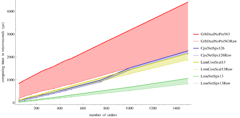
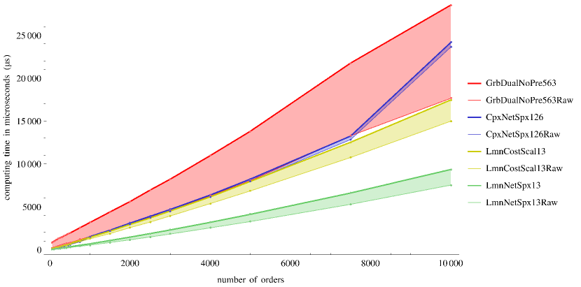
Figure 1: Computing times for $3000$ random instances with $20$ contracts/nodes and a varying number of orders/arcs. The wide bars represent the model creation times. The thick marked upper borders of these bars represent the total computing times and the thin marked lower borders represent the raw computing times.

The two graphs in Figure 1 display the average computing time for instances with 20 contracts/nodes and a varying number of orders/parallel arcs. Each data point represents the average computing time of 50 random-instances. The instances are solved as follows: At first we load the raw instance parameters into the memory (RAM). Then, in the model creation phase, we create and load an instance of (LP3) with scaling factor $G:=2|T|+1$ into the memory of the respective solver via its application programming interface (API). Next, in the raw computing phase, we call the solver routine that starts the computations, we import the results via the API, and finally compute the prices as described in equation (23).

Figure 1 shows that in our test cases, the Lemon network simplex clearly outperforms the other three algorithms. For example, its average computing time for instances with $1000\text{\,}$ orders amounts to only $678\text{\,}\text{$\upmu$s}$, whereas Gurobi’s dual simplex requires $3168\text{\,}\text{$\upmu$s}$; on average, instances with 10,000 orders are solved in $9.3\text{\,}\mathrm{ms}$, whereas Gurobi requires $28.5\text{\,}\mathrm{ms}$. The long total computing times of Gurobi are basically due to the fact that the creation of the LP model requires a lot of time. In contrast to Gurobi, CPLEX provides a network API that allows for a fast model creation. Due to this fast API, the CPLEX network simplex easily outperforms Gurobi’s dual simplex. Nevertheless, the Lemon cost scaling is still slightly faster than the CPLEX network simplex. We would like to stress, though, that the cost scaling algorithm is actually not a valid subroutine for Algorithm 1, as it provides arbitrary optimal solutions and does not provide the required optimal extreme points. We included this algorithm mainly for the sake of comparison.

Apart from the significantly shorter computing times, the Lemon network simplex has further advantages in comparison to CPLEX and Gurobi: as it is open source the source code can be readily modified. Moreover, it uses exact arithmetic without any numerical errors, whereas CPLEX and Gurobi use floating point operations, which are exposed to small numerical errors. These numerical errors though are of secondary importance as they can be safely ignored: due to optimal solutions being integral, rounding a flawed fractional basic solution yields the correct integral basic solution.

Comparison of Algorithms 1 to 5 on real-world instances

We will now compare the running times of Algorithms 1 to 5. For each algorithm we present numerical results of the algorithm variant that uses the CPLEX network simplex as a subroutine. In the previous section, we used different standard solvers as subroutines for Algorithm 1 (weighted objective) and observed that the Lemon network simplex is in all likelihood the best solver for this task (see Figure 1). However, in this section, Algorithms 4 and 5 require an LP solver as subroutine. For this reason, we decided to use the CPLEX network simplex for all five algorithms in our comparison.

In this test, we solved 40 real-world instances with each algorithm. The instances were generated from historical order books of EUREX and were initially studied by Winter et al (2011). The proposed solution approach therein is an integer programming model solving the futures opening auction problem. For completeness, we would like to mention that the original data set has 55 instances, however only for 40 instances the order books could be fully reconstructed, which is necessary for a comparison.

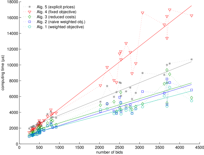
Figure 2: Comparison of five different algorithms.

Figure 2 shows the computing times of Algorithm 1 to 5. The figure suggests that the computing time is roughly linear in the number of orders, which is also consistent with the results in Section 5.2. Furthermore, we can see that Algorithm 4 (fixed objective) is the slowest one. The second slowest algorithm is Algorithm 5 (explicit prices) as its price computation via (LP4) is very time consuming. The computing times of the other three algorithms are the shortest ones and are more or less similar.

Table 1: Computing times for 40 real instances

		Computing time in $\text{\,}\text{$\upmu$s}$ (average of 10 runs per instance)
		Weighted	Naive	Reduced	Fixed	Explicit
		objective	weighted obj.	costs	objective	prices
		1 LP	1 LP	2 LPs	2 LPs	2 LPs	IP model
#	Bids	Alg. 1	Alg. 2	Alg. 3	Alg. 4	Alg. 5	Winter et al (2011)
1	246	937	931	1120	1464	1947	270000
2	300	1115	1095	1307	1729	2121	80000
3	324	1037	1060	1231	1666	2112	70000
4	334	1161	1101	1629	1841	2157	750000
5	336	1170	1106	1386	1947	2140	970000
6	342	1102	1139	1290	1757	2251	90000
7	361	1184	1148	1449	1909	2273	530000
8	393	1192	1180	1387	1880	2167	500000
9	443	1186	1193	1387	1904	2360	210000
10	445	1511	1442	1894	2305	2520	340000
11	478	1821	1744	2056	2621	2477	120000
12	491	1473	1512	1661	2488	2786	140000
13	496	1807	1736	2227	2956	2829	250000
14	505	1355	1364	1555	2137	2468	110000
15	516	1441	1437	1871	2322	2665	630000
16	518	1695	1637	2215	2690	2608	700000
17	555	1774	1809	2076	2645	2327	130000
18	614	1747	1685	1941	2997	2871	220000
19	701	2277	2303	2640	3530	3769	80000
20	787	2454	2643	3117	4336	4071	480000
21	794	2363	2457	2821	3705	3360	110000
22	833	2132	2063	2943	3885	3399	110000
23	917	2155	2113	2416	3934	3307	8220000
24	2023	4354	4105	4906	7404	5340	30000
25	2190	4470	5089	5066	9720	7328	90000
26	2361	3828	4154	5345	8046	5957	100000
27	2424	3925	3869	4112	7788	6557	1270000
28	2502	4271	5907	4612	11424	7782	110000
29	2530	5180	5250	6536	11706	7710	220000
30	2537	3787	4089	4311	10686	6083	120000
31	2663	4244	4522	4806	12753	6650	5330000
32	2767	4286	4947	4656	11623	7130	450000
33	2812	3877	3853	4358	8922	5678	50000
34	2906	4446	4449	4734	10205	6465	150000
35	3074	4693	6626	5067	16617	8976	11970000
36	3616	6072	6431	7611	15096	8746	1200000
37	3683	7731	8211	9356	16172	10004	350000
38	3684	4764	4960	5172	13393	7731	40000
39	3751	7156	7785	8831	16996	10173	70000
40	4298	5458	6829	5844	16254	10701	70000
avg.	1539	2966	3174	3474	6586	4750	918250

Table 1 presents the average computing times of the five algorithms and the one of Winter et al (2011). Note that the computing times of Winter et al (2011) are not directly comparable as the computations where performed on a slower machine and with a different solver. However, the table shows that this method is the slowest one by a huge margin so that the difference in hard- and software is negligible. The fastest method is Algorithm 1 (weighted objective). Its average computing time amounts to only $2966\text{\,}\text{$\upmu$s}$. Furthermore, we see that Algorithm 3 (reduced costs) is a reasonable alternative to Algorithm 1, since its average computing time of $3474\text{\,}\text{$\upmu$s}$ is only slightly longer but it is numerically more robust, as it does not scale the objective.

Furthermore, we can observe that the running time of the CPLEX network simplex depends on the size of the scaling factor: the smaller the factor, the shorter the running time (see Table 1). The polynomial network simplex variant of Orlin (1997) behaves in a qualitatively similar way. It runs in

$$O\left(\min\{|T|^{2}|I|\log|T|C,\ |T|^{2}|I|^{2}\log|T|\}\right)$$

time, where $C$ is the largest absolute objective coefficient.

Arbitrage example

We now provide an example where the new model yields a higher surplus, a higher liquidity, and a better price quality than the old one. Moreover, we show how an arbitrage trader can make a risk free profit in this situation.

Example 3

Assume that there are three orders in the order books:

1. Buy 1 gold contract with delivery in June; Limit price: $1072\text{\,}\mathrm{U}\mathrm{S}\mathrm{D}$.
   $\quad Q_{1}=(1,0)^{\top}\quad p_{1}=(1072,0)$

2. Sell 1 gold contract with delivery in August; Limit price: $1068\text{\,}\mathrm{U}\mathrm{S}\mathrm{D}$.
   $\quad Q_{2}=(0,-1)^{\top}\quad p_{2}=(0,1068)$

3. Sell 1 gold combination $\{\text{June, August}\}$; Limit price: $1\text{\,}\mathrm{U}\mathrm{S}\mathrm{D}$.
   $\quad Q_{3}=(-1,1)^{\top}\quad p_{3}=(1,0)$

The old auction model would not match any contracts as it would perform a separate auction for each product. The total surplus would amount to $0\text{\,}\mathrm{U}\mathrm{S}\mathrm{D}$ and the exchange would not publish any market clearing price because no order was executed. In the new model, all three orders can be matched. The total surplus amounts to $3\text{\,}\mathrm{U}\mathrm{S}\mathrm{D}$ and the exchange would, for example, publish the following market clearing prices:

• June: $\pi_{\text{Jun}}=$1069\text{\,}\mathrm{U}\mathrm{S}\mathrm{D}$$,

• August: $\pi_{\text{Aug}}=$1068\text{\,}\mathrm{U}\mathrm{S}\mathrm{D}$$,

• $\{\text{June, August}\}$: $\pi_{\text{Jun}}-\pi_{\text{Aug}}=$1\text{\,}\mathrm{U}\mathrm{S}\mathrm{D}$$.

This solution is preferred to the zero solution since it increases the liquidity and price quality. Now assume that an arbitrage trader looks at the order books and submits the following three additional orders immediately before the auction starts:

1. Sell 1 gold contract with delivery in June; Limit price: $1072\text{\,}\mathrm{U}\mathrm{S}\mathrm{D}$.
   $\quad Q_{1}=(-1,0)^{\top}\quad p_{1}=(1072,0)$

2. Buy 1 gold contract with delivery in August; Limit price: $1068\text{\,}\mathrm{U}\mathrm{S}\mathrm{D}$.
   $\quad Q_{2}=(0,1)^{\top}\quad p_{2}=(0,1068)$

3. Buy 1 gold combination $\{\text{June, August}\}$; Limit price: $1\text{\,}\mathrm{U}\mathrm{S}\mathrm{D}$.
   $\quad Q_{3}=(1,-1)^{\top}\quad p_{3}=(1,0)$

In the old model, all 6 orders would be executed and the surplus of each product auction would be zero, but the arbitrage trader would end up with a risk free profit of $3\text{\,}\mathrm{U}\mathrm{S}\mathrm{D}$ (minus trading fees, e.g.: $3\cdot$0.7\text{\,}\mathrm{U}\mathrm{S}\mathrm{D}$$). The exchange would publish the following inconsistent prices:

• June: $\pi_{\text{Jun}}=$1072\text{\,}\mathrm{U}\mathrm{S}\mathrm{D}$$,

• August: $\pi_{\text{Aug}}=$1068\text{\,}\mathrm{U}\mathrm{S}\mathrm{D}$$,

• $\{\text{June, August}\}$: $1\text{\,}\mathrm{U}\mathrm{S}\mathrm{D}$, which differs from $\pi_{\text{Jun}}-\pi_{\text{Aug}}=$4\text{\,}\mathrm{U}\mathrm{S}\mathrm{D}$$.

In the new model, the additional orders of the arbitrage trader would not be executed and would not affect the outcome of the auction.

Summary

We introduced several new methods for solving the futures opening auction problem. We showed that the problem can be modeled as a min cost flow problem with two hierarchical objectives. The primary objective is the surplus maximization and the secondary one is the volume maximization. This kind of problem can be solved efficiently by exploiting the properties of extreme point solutions, as it is done in Proposition 2 and Theorem 4.1. The resulting algorithm is very simple as it just computes a pair of primal dual optimal extreme points of a min cost flow problem with a weighted objective and then scales and rounds the dual solution. However, it is not only the simplest algorithm but also turned out to be the fastest one in our numerical tests. In those tests we also compared different standard solvers for solving the underlying optimization problems. The results suggest that the Lemon network simplex is the fastest one for this task. Due to the short computing times, our algorithm (with Lemon as a subroutine) is well suited for real-world applications.