Improved Moving Puncture Gauge Conditions for Compact Binary Evolutions

Abstract

Robust gauge conditions are critically important to the stability and accuracy of numerical relativity (NR) simulations involving compact objects. Most of the NR community use the highly robust—though decade-old—moving-puncture (MP) gauge conditions for such simulations. It has been argued that in binary black hole (BBH) evolutions adopting this gauge, noise generated near adaptive-mesh-refinement (AMR) boundaries does not converge away cleanly with increasing resolution, severely limiting gravitational waveform accuracy at computationally feasible resolutions. We link this noise to a sharp (short-wavelength), initial outgoing gauge wave crossing into progressively lower resolution AMR grids, and present improvements to the standard MP gauge conditions that focus on stretching, smoothing, and more rapidly settling this outgoing wave. Our best gauge choice greatly reduces gravitational waveform noise during inspiral, yielding less fluctuation in convergence order and $\sim 40\%$ lower waveform phase and amplitude errors at typical resolutions. Noise in other physical quantities of interest is also reduced, and constraint violations drop by more than an order of magnitude. We expect these improvements will carry over to simulations of all types of compact binary systems, as well as other $N$+1 formulations of gravity for which MP-like gauge conditions can be chosen.

I Introduction

With the first direct observations of incident gravitational waves (GWs) expected in only a few years, an exciting new window on the Universe is about to be opened. But our interpretation of these observations will be limited by our understanding of how information about the GW sources is encoded within the waves themselves. The parameter space of likely sources is large, and compact binary systems consisting of two black holes (BHs), two neutron stars, and one of each are likely to be the most promising sources. However, filling this parameter space with the corresponding theoretical gravitational waveforms through merger—when GWs are strongest and many binary parameters are most distinguishable—will require a large number of computationally expensive numerical relativity (NR) simulations.

At the heart of the computational challenge lies an arguably even greater theoretical one, which seeks to find an optimal approach for solving Einstein’s equations on the computer. These approaches generally decompose the intrinsically four-dimensional set of Einstein’s field equations into time-evolution and constraint equations—similar to Maxwell’s equations Baumgarte and Shapiro (2010). Once the data on the initial 3D spatial hypersurface are specified, the time-evolution equations are repeatedly evaluated, gradually building the four-dimensional spacetime one 3D hypersurface at a time. Einstein’s equations guarantee the freedom to choose coordinates in the 4D spacetime, and these are specified via a set of gauge evolution equations. Devising robust gauge conditions, particularly when black holes inhabit the spacetime, has been a problem at the forefront of NR for decades. In fact, discovery of gauge conditions leading to stable evolutions in the presence of moving black holes played a large role in the 2005 numerical relativity revolution, culminating in the first successful binary black hole (BBH) inspiral and merger calculations Pretorius (2005); Campanelli et al. (2006); Baker et al. (2006a).

The most widely adopted formulation for compact binary evolutions is the highly robust “BSSN/moving puncture” (hereafter BSSN/MP) formulation Campanelli et al. (2006); Baker et al. (2006a), which combines the Baumgarte-Shapiro-Shibata-Nakamura (BSSN) 3+1 decomposition of Einstein’s equations Nakamura et al. (1987); Shibata and Nakamura (1995); Baumgarte and Shapiro (1999) with the “moving puncture” (MP) gauge conditions that implement the 1+log/$\Gamma$-freezing gauge evolution equations Alcubierre et al. (2003); van Meter et al. (2006). It has been about a decade since BSSN/MP was first developed, and it remains in use by much of the NR community, largely unmodified. This is a testament to the robustness of the MP gauge choice, as well as the difficulties associated with devising stable techniques for evolving spacetimes containing BHs.

The BSSN/MP equations are typically solved on the computer with high-order finite-difference approaches on adaptive-mesh refinement (AMR) numerical grids Zlochower et al. (2005); Baker et al. (2006b); Brügmann et al. (2008); Campanelli et al. (2007); Herrmann et al. (2007); Sperhake (2007); Etienne et al. (2008); Pollney et al. (2007, 2011). Such grids are essential for computational efficiency, as the simulation domain must be hundreds to thousands of times larger than the initial binary separation to causally disconnect the outer boundary from the physical domain of interest for the duration of the simulation. This effectively prevents errors linked to the enforcement of approximate outer boundary conditions from propagating inward and lowering the convergence order of our gravitational waveforms. In addition, very high resolution must be used in the strongly curved spacetime near the BHs, while resolution requirements are much lower far from the binary, where GWs with wavelengths of order $10M$ must be accurately propagated ($M$ is the total ADM mass of the system). Thus, AMR grids in MP calculations typically resolve the strong-field region best, with progressively lower resolutions away from this region to the outer boundary. Typical gridspacings at the outer boundary can be $\sim 1000$ times larger than in the strong-field region.

The BSSN/MP+AMR paradigm has been most thoroughly tested in the context of BBH evolutions, and a large number of theoretical BBH GWs have been produced with this paradigm that widely sample parameter space (e.g., Lousto and Zlochower (2014); Pekowsky et al. (2013); Hinder et al. (2013)). However, when the BSSN/MP+AMR paradigm is pushed to very high accuracies or to difficult regions of BBH parameter space, it has been found (e.g., Zlochower et al. (2012)) to yield inconsistent gravitational waveform convergence with increasing resolution, making error estimates difficult, and effectively limiting waveform accuracy. In Zlochower et al. (2012) it was hypothesized that these convergence issues might be linked to noise from high-frequency waves generated at grid refinement boundaries.

This is a compelling hypothesis, especially in light of Fig. 1, which shows regularly-spaced spikes in L2 norm Hamiltonian constraint violations on a logarithmic time scale. Interestingly, the onset of each spike in this BBH evolution is timed almost perfectly to grid refinement crossings of a wave that starts from the strong-field region at the onset of the calculation and propagates outward superluminally at speed $\sqrt{2}c$ (vertical lines). This propagation speed is a smoking gun, as linearized analyses Alcubierre (2003) indicate only one propagation mode with that speed in the standard BSSN/MP formulation. This mode primarily involves the lapse and is governed by the lapse evolution gauge condition. The connection between spikes in Hamiltonian constraint violations and the initial outgoing lapse wave has been noted previously Baker et al. (2006b).

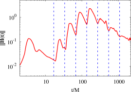
Figure 1: L2 norm of Hamiltonian constraint violation $||\mathcal{H}(t)||$ outside black hole horizons (Eq. 18), versus time (solid red curve), for “standard” BSSN/MP+AMR BBH calculation. Dashed blue vertical lines denote the times at which an outgoing wave traveling at $\sqrt{2}c$—starting from the origin at the onset of the calculation—encounters a grid refinement boundary.

Expanding on this idea, we note that all BSSN evolution equations are coupled to the lapse and its derivatives, so noise from reflections in this gauge quantity can be easily converted into noise in physical modes (e.g., noise in GWs) and even constraint violations. Further, differencing errors from the part of the wave that is transmitted into the coarser grid are converted into constraint violations and errors in non-gauge waves as well. We expect improved resolution would mitigate this problem, but even a factor of two increase—the typical range in most BSSN/MP convergence studies—would enable evolution of a sharp (short-wavelength) feature through only one additional coarser level before it succumbs to dissipation through under-resolution. Additionally, it is likely that zero- or low-speed modes in Hamiltonian constraint violations (see, e.g., Gundlach and Martín-García (2004)) may exacerbate any errors generated as the initial sharp lapse wave propagates into a coarse grid.

Since sharp features in the initial outgoing lapse wave are likely responsible for spikes in Hamiltonian constraint violations, as well as noise and other errors in physical quantities, we can conceive of at least two strategies for mitigating this effect: (1) adjusting the initial conditions to minimize gauge dynamics, in a similar vein to Hannam et al. (2009), or (2) modifying the standard MP lapse evolution equation so that the initial sharp outgoing lapse wave is stretched and smoothed as it propagates outward from the binary. We chose the latter strategy. Strikingly, we find our stretching and smoothing modifications to the lapse evolution equation are sufficient to reduce constraint violations by more than an order of magnitude, confirming our hypothesis, except near the beginning of our calculations, where early-time spikes in constraint violations remain.

We remove these stubborn spikes by initially reducing the timestep on the BSSN field equations by a factor of $\sim 10^{3}$, while the gauge evolution equations are evolved according to the original time coordinate. This time reparameterization technique increases the gauge wave speeds to about 30 times the coordinate speed of light, allowing the gauge evolution to very quickly relax near $t=0$ in response to the physical fields. As the gauge fields relax, evolution of the BSSN field variables is slowly accelerated so that their timestep matches that of the MP gauge evolution, after about $10M$ of evolution in the un-reparameterized time coordinate. We show this time reparameterization is, on an analytic level, equivalent to a time-dependent rescaling of the lapse and shift, leaving the BSSN field equations unmodified in the reparameterized time coordinate.

When combined, these gauge improvements significantly reduce constraint violations from the onset of the calculation through BBH merger. For example, the L2 norm Hamiltonian constraint violation outside the BHs is reduced on average by a factor of 20 at $t>0$ at lowest resolution. Hamiltonian constraint violations converge at a much higher order in the presence of our improved gauge conditions, so this factor increases to $\sim 50$ at the highest resolutions attempted.

Turning to gravitational waveforms, we find that in the “standard” BSSN/MP+AMR paradigm, noise appears to dominate GW power at wave periods $\sim 10M$, and this spike in power does not diminish with increasing resolution. Meanwhile, our “best” gauge choice appears to drop this noise-generated GW power spike by about an order of magnitude, and its power spectrum at short wave periods does drop with increasing resolution. In conjunction with this removal of waveform noise—and perhaps most significantly—we find that gravitational waveform convergence is far cleaner when using the new techniques, enabling more reliable Richardson extrapolations and possibly paving the way to higher accuracies than the standard BSSN/MP+AMR paradigm might allow. In fact, our “best” gauge choice reduces Richardson-extrapolation-based error estimates of GW phase and amplitude error during inspiral by about 40–50%. However, we observe in these waveforms that only the phase error is reduced significantly at merger.

Our gauge improvements are presented exclusively in the challenging context of an 11-orbit, equal-mass BBH calculation in which one BH is nonspinning and the other possesses a spin of dimensionless magnitude 0.3, aligned with the orbital angular momentum. Despite our focus on a single physical scenario, we expect these new techniques will improve the accuracy and reliability of simulations couple the MP+AMR paradigm to BSSN and other $N$+1 NR formulations (e.g., Bona et al. (2003); Gundlach et al. (2005); Bernuzzi and Hilditch (2010); Zilhão et al. (2011)), not only for BBH and single-BH evolutions, but also for binary systems with matter, such as neutron star–neutron star and black hole–neutron star binaries. Finally, we anticipate that careful reparameterization of the time coordinate when the gauge and physical quantities change most significantly—both at the beginning of evolutions and during merger—may help stabilize compact binary simulations, making it easier to cover difficult regions of parameter space.

The rest of the paper is organized as follows. Section II summarizes our basic equations and gauge improvements, Sec. III outlines numerical algorithms and techniques, Sec. IV details results from these improved gauge conditions, and Sec. V summarizes both our conclusions and plans for future improvements.

II Basic Equations

In the following sections, all quantities are given in geometrized units: $G=c=1$. Also, with the exception of Sec. III, we designate quantities in terms of $M$, the total initial ADM mass of our binary.

II.1 Initial Data

The Bowen-York initial data Bowen and York Jr. (1980); Brandt and Brügmann (1997) prescription is used to generate an equal-mass, low-eccentricity BBH system approximately 11 orbits prior to merger. One BH is nonspinning, and the other is spinning with initial spin parameter $0.3$ aligned with the orbital angular momentum. We choose this case because it (1) avoids many of the symmetries of an equal-mass, aligned-spin system (though is still symmetric about the orbital plane), (2) requires a significantly long inspiral calculation to merger, and (3) is one of the cases featured by the Numerical Relativity/Analytical Relativity (NRAR) NRA ; Hinder et al. (2013) collaboration (NRAR case label U1+30+00 in Hinder et al. (2013)).

We adopt standard initial values for the lapse and shift, choosing $\beta^{i}(t=0)=0$ and $\alpha(t=0)=\Psi^{-1}_{\text{BL}}$, where $\Psi_{\text{BL}}$ is the Brill-Lindquist conformal factor (Eq. 5 in Brügmann et al. (2008)). We devised other choices for initial lapse and shift that more closely approximate their final, relaxed values. These choices either had no effect or resulted in amplified constraint violations. We attribute this to the fact that in the process of settling, the gauge responds to early gravitational-field dynamics, and vice versa. Thus if one wishes to minimize early gauge dynamics, a different strategy for specifying the initial gauge that accounts for the early $t>0$ evolution of the spacetime might be more effective.

II.2 Evolution Equations and Diagnostics

II.2.1 Evolution Equations for Gravitational Fields

We employ the standard set of BSSN equations for gravitational field evolution Baumgarte and Shapiro (1999), except $W=e^{-2\phi}$ van Meter (2006); Marronetti et al. (2008) is chosen as the evolution variable instead of the original BSSN conformal variable $\phi$. Such a choice or variant thereof (e.g., $\chi=W^{2}$; see Hinder et al. (2013) for other possibilities) is motivated by the the fact that finite-difference techniques generally approximate functions by overlapping polynomials when taking derivatives, and $W$ (or $\chi$) is better approximated by polynomials than $\phi$, particularly in the strong-field region ($\phi\to\infty$ at black-hole punctures). Thus choosing $W$ or $\chi$ as an evolution variable results in less truncation error at a given resolution than using $\phi$.

II.2.2 Reparameterization of the Time Coordinate

We present a new modification of the BSSN/MP equations, originally aimed at reducing an early spike of constraint violations in our BBH evolutions. Understanding one source of these violations requires some insights into how our AMR driver Carpet Schnetter et al. (2004) works.

AMR drivers are generally faced with the problem of interpolating data between grids at different resolutions. Carpet solves this problem by interpolation (prolongation) in both space and time. Suppose we wish to evolve data on a fine (high-resolution) AMR grid with spatial resolution $\Delta x$ from time $t$ to $t+\Delta t$. Also suppose data already exist on the surrounding coarser grid with spatial resolution $2\Delta x$ at $t$ and $t\pm 2\Delta t$. After the fine grid has been updated, Carpet needs to fill the buffer cells between the fine and coarser levels. However, data do not exist on the coarser level at $t+\Delta t$, so coarse-grid data at $t$ and $t\pm 2\Delta t$ are interpolated in space and time to provide data at $t+\Delta t$.

At the start of the calculation, the initial data solver provides data at only a single time, $t=0$, but we have chosen second-order time interpolation to fill buffer zones at grid refinement boundaries. Thus we need data at three timesteps to proceed. Carpet offers two algorithms for filling in these two missing timesteps. The first is to simply copy the data from $t=0$, and the second evolves data at $t=0$ backward and forward in time to fill them in. The latter technique reduces truncation errors at a higher order of convergence than the former, but constraint violations in either case just after the evolution begins will generally be much larger than at $t=0$, as the initial data are extremely accurate and are usually generated on high-resolution spectral grids.

To mitigate the errors at the start of the calculation, we choose to copy the data from $t=0$ and reparameterize the time coordinate so that the timesteps near $t=0$ are incredibly small, compared to our original time coordinate. The coordinate timestep then very gradually and smoothly grows to the usual value. In particular, we find the following prescription works well.

All the BSSN/MP evolution equations can be written in the following form:

$$\partial_{t}\mathcal{E}={\rm RHS},$$ (1)

where $\mathcal{E}$ is any of the evolved variables, $\partial_{t}$ denotes the usual partial time-derivative and RHS the right-hand side of the evolution equation. Our first time reparameterization scheme, which we call “TR1”, simply multiplies every “RHS” by

$$f(t)=\operatorname{Erf}(t;10,5).$$ (2)

Here, we define $\operatorname{Erf}(x;x_{0},w)$ as follows

$$\operatorname{Erf}(x;x_{0},w)=\frac{1}{2}\left[\operatorname{erf}\left(\frac{x-x_{0}}{w}\right)+1\right],$$ (3)

where $\operatorname{erf}(x)$ is the standard, $C^{\infty}$ error function, $x_{0}$ marks the center of the error function distribution and $w$ the width.

Note that although $f(t)$ yields extremely small timesteps early in the evolution, the timesteps return to the fiducial value ($f(t)\to 1$) smoothly and rapidly. The net effect of TR1 is an increase in total wallclock time of only $0.5\%$ for our 11-orbit BBH calculations, equivalent in cost to evolving without time reparameterization an additional $11M$. Though our time reparameterization techniques do appear to modify the RHS of the BSSN field equations, we demonstrate in Appendix A that Einstein’s equations are still satisfied, as both of our time reparameterization techniques are in fact equivalent to gauge choices.

Using our “TR1” strategy, the initial timestep is $\sim 10^{-3}$ times the initial timestep without time reparameterization, and we observe a significant reduction in evolution errors when compared to copying the initial data alone without time reparameterization, particularly in the momentum constraint. This finding is demonstrated in Sec. IV.

Though our main objective in reparameterizing the time coordinate was to reduce errors induced by copying data from $t=0$ to earlier times, we find we can reduce errors at early times significantly more by choosing not to reparameterize time in the gauge evolution equations (i.e., the lapse and shift). We call this our “second” time reparameterization choice, or “TR2”. TR2 increases the characteristic speeds of the lapse evolution equation, of order 30 times the coordinate speed of light initially . The net effect is accelerated evolution of the gauge relative to the gravitational fields, causing the coordinates to relax much faster.

We apply two other major modifications to the gauge evolution equations, including one aimed at stretching outgoing gauge waves and another focused on adding dissipation terms that significantly reduce short-wavelength noise. These modifications are described in the next section.

II.2.3 Gauge Evolution Equations

The usual MP gauge-evolution equations consist of the “Gamma-driver” shift condition Alcubierre et al. (2003), of which we choose the first-order “nonshifting-shift” variant van Meter et al. (2006), and the 1+log slicing condition for the lapse Alcubierre et al. (2003).

$$\partial_{t}\beta^{i} = \frac{3}{4}\tilde{\Gamma}^{i}-\eta\beta^{i},\ \ \ \eta=1.375$$ (4)

$$\partial_{t}\alpha = \beta^{i}\partial_{i}\alpha-2\alpha K.$$ (5)

We refer to these gauge conditions as the “OldGauge”. The motivation behind this 1+log slicing condition becomes apparent when combined with the evolution equation for $K$, the trace of the extrinsic curvature,

$$\partial_{t}K=\beta^{i}\partial_{i}K-D^{i}D_{i}\alpha+\alpha\left(\tilde{A}_{ij}\tilde{A}^{ij}+\frac{1}{3}K^{2}\right).$$ (6)

Taking a time-derivative of Eq. (5), combining with Eq. (6), and keeping only the principal parts yields

$$\partial_{t}^{2}\alpha\simeq 2\alpha\gamma^{ij}\partial_{i}\partial_{j}\alpha,$$ (7)

a wave equation with wave speed $\sqrt{2\alpha}$ (see also Alcubierre (2003)).

As mentioned previously, our strategy is based on the observation that the sharp initial outgoing lapse wave appears to generate spikes in the time evolution of the L2 norm of the Hamiltonian constraint violations when it crosses coarser and coarser AMR grid-refinement boundaries. Thus we focus on modifying the 1+log slicing condition for the lapse to stretch this initial wave packet, as well as damp short-wavelength noise in $\alpha$ generated by grid refinement boundary crossings. Gauge freedom guarantees our ability to do this, and the job is made easier by its interpretation as a wave equation (Eq. 7). We review our improvements to the 1+log slicing condition below.

Our improved 1+log slicing condition is as follows

$$\partial_{t}\alpha={\underbrace{\textstyle f(t)\beta^{i}\partial_{i}\alpha}_{\text{Term (1)}}}-{\underbrace{\textstyle g(t,r)\alpha K}_{\text{Term (2)}}}+{\underbrace{\textstyle h(r)\nabla_{\rm flat}^{2}\alpha}_{\text{Term (3)}}}+\text{KO}.$$ (8)

Here $r=\sqrt{x^{2}+y^{2}+z^{2}}$. We now specify the unknown functions and explain each term.

Term (1): $f(t)=f_{0}(t)\equiv\operatorname{Erf}(t;10,5)$ (consistent with Eq. (2)). Note that this is the only term in the lapse condition that is multiplied by $f(t)$ in the TR2 time reparameterization, while all other RHS terms in Eq. 8 are multiplied by $f(t)$ as well in TR1.

Term (2): As in Eq. (7), $\sqrt{g(t,r)\alpha}$ provides the wave speed. We stretch outgoing lapse waves by making $g(t,r)$ a monotonically increasing function of coordinate radius $r$ (i.e., by accelerating the wave as it propagates outward). In so doing, one must be careful to avoid exceeding the maximum local speed allowed by the local Courant-Friedrichs-Lewy (CFL) condition on each AMR grid. In practice, however, this is not a highly restrictive constraint, as the shift evolution equation’s $\eta$ term (4) also sets a stringent upper bound on the timestep Schnetter (2010), forcing us to evolve the outermost AMR levels with a very small timestep anyway. So without significant modification of current techniques, we may already stably evolve waves in the outer regions of our grid that propagate much faster than the local coordinate speed of light. This enables us to choose the lapse acceleration function $g(t,r)$ to be a steeply increasing function of $r$, and we are careful to select a function that is easily extensible to arbitrary binary separations, choosing the following functional form:

$$g_{0}(r) \equiv v_{i}+(v_{o}-v_{i})\operatorname{Erf}(r;x_{1},w_{1})$$

$$+re^{-4.42}\operatorname{Erf}(r;x_{2},w_{2}),$$

where we set inner wave speed $v_{i}=2$, outer wave speed $v_{o}=8$, $x_{1}=30$, $w_{1}=10$, $x_{2}=130$, and $w_{2}=15$. The variable $x_{1}$ may be adjusted proportionally up (down) for binaries with larger (smaller) initial separations. Figure 2 shows how this function satisfies the CFL condition $\sqrt{g(t,r)}<\Delta x/\Delta t$ on all grids. Notice that this choice leads to a safety factor $\Delta x/\Delta t/\sqrt{g(t,r)}$ of $\sim 2-50$ that reduces errors in time and ensures that a moving AMR grid (tracking the trajectory of a BH) does not cross into a CFL-unstable region. Notice also that when the lapse wave hits the outer boundary, its coordinate speed is nearly $10$. In principle, outer boundary conditions should be adopted to accommodate this radially dependent superluminal speed, though our outer boundary conditions for the lapse were not adjusted for the runs presented here, with no apparent ill effects.

The left panel of Fig. 3 plots lapse along the $x$-axis at different times, demonstrating that choosing $g(r,t)=g_{0}(r)$ instead of the standard choice $g(r,t)=2$ stretches the initial outgoing lapse wave. The red-solid curve shows the initial lapse (the puncture is located at $x/M\approx 6$), and the cyan dash-dotted curve the final, settled lapse. The other curves demonstrate how the initial lapse wave settles as it propagates away from the strong-field region (direction of propagation shown by black arrow). In particular, we find the outgoing lapse wave indeed possesses sharp features. Also, in the OldGauge case, the wave front crosses $r=140M$ at $t\approx 100$, corresponding to a propagation speed of very nearly $\sqrt{2}$, consistent with the linear analysis of the lapse evolution equation. Notice that the choice $g(r,t)=g_{0}(r)$ does in fact accelerate and stretch the initial outgoing lapse pulse, leading the wavefront to the same location as the OldGauge case in about half the time.

We explore another realization of $g(t,r)$, which, independent of other terms in Eq. (8), introduces a time dependence:

$$g_{1}(t,r) \equiv [v_{i}(t)+(v_{o}-v_{i}(t))\operatorname{Erf}(r;x_{1},w_{1})]$$

$$+re^{-4.42}\operatorname{Erf}(r;x_{2},w_{2}).$$

Here, all parameters are as in $g_{0}(r)$, except the inner wave speed $v_{i}$ is chosen to be a function of time,

$$v_{i}(t)=0.5+1.5\operatorname{Erf}(t;40,10).$$ (11)

Notice that at early times, $v_{i}(t)\approx 0.5$, yielding sub-luminal lapse speeds in the inner region, providing a greater stretch, and at times $t\gtrsim 40$, $v_{i}(t)$ rapidly increases to $2.0$, which brings $g_{1}(t,r)\to g_{0}(r)$. We have attempted evolutions that maintain sub-luminal lapse speeds in the inner region, and Hamiltonian constraint violations are significantly reduced. However, maintaining sub-luminal lapse speeds also resulted in a large increase in the BHs’ irreducible masses as well as a very strong spike in constraint violations near merger, perhaps due to a gauge shock (see, e.g., Alcubierre (2003)).

We also attempted a much steeper function for $g(t,r)$ in the outer regions, keeping a more constant safety factor, leading to wave speeds $\sim 100$ at the outer boundary. This greatly reduced constraint violations (Hamiltonian constraint in particular) through much of the inspiral, but the constraints spiked after the lapse wave returned from the outer boundary and crossed into the strong-field region. No such reflection was observed with $g_{0}(r)$ or $g_{1}(t,r)$, as we anticipate that the much slower lapse wave speeds near the outer boundary enabled dissipation terms to act longer and more effectively, resulting in significantly less reflection.

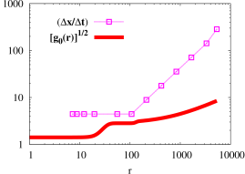
Figure 2: Local lapse speed parameter $\sqrt{g_{0}(r)}$ (solid red line), as compared to the maximum allowed speed by the CFL condition at each AMR level’s most distant point from the origin, at $t=0$ (magenta squares). Note that this curve is indistinguishable from $g_{1}(t\gtrsim 50,r)$, as $g_{1}(t,r)\to g_{0}(r)$ rapidly at $t>40$. Note also that in cases for which time reparameterization techniques are applied, $t$ refers to the reparameterized time coordinate.

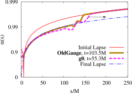
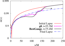
Figure 3: Effect of replacing the lapse speed factor of $2$ in the “standard” BSSN/MP 1+log slicing condition (OldGauge, Eq. 5) with other functions. Left panel: Evolved OldGauge lapse along $x$-axis after $\approx 100M$ of evolution (thick solid brown) is compared with the g0 lapse (thick dashed magenta) as it crosses the same position, at $t\approx 55M$. For comparison, initial lapse (thin solid red) is plotted alongside the settled lapse of the merged BH remnant (thin dot-dashed blue). The black arrow shows the direction of lapse wave propagation. Right panel: Same as left panel, except the g0 case (thick dashed magenta) is compared to our “best” gauge choice BestGauge (g1+TR2+h+d5d7); thick solid gray; see Table 1 for full details).

Term (3): The flat-space Laplacian acts as a dissipative filter that damps high-frequency oscillations. These oscillations include the sharp features in the problematic wave pulse, and may include noise resulting from reflections or interpolation errors at refinement boundaries. In constructing an $h(r)$ for our AMR grids, care must be taken so that the following numerical stability criterion for parabolic terms will be satisfied:

$$h(r)\lesssim\frac{1}{6}\frac{(\Delta x)^{2}}{\Delta t},$$ (12)

where $\Delta x=\Delta y=\Delta z$ is assumed, consistent with our numerical grids. This is not a strict inequality, as it was derived from a CFL analysis of the standard heat equation, using centered second-order finite-differencing and Euler time integration. Our numerical scheme is more sophisticated, so we reduce $h(r)$ so that the inequality is comfortably satisfied. In addition, $\Delta t/\Delta x$ is held fixed as we vary $\Delta x$ in our resolution studies, so with sufficiently high resolution and $h(r)>0$, the above inequality will always be violated for explicit time integration. To protect against this, $h(r)$ is reduced even more when higher resolution is deemed necessary. In general, we choose $h(r)$ such that it is roughly $1/100$ the right-hand side of the inequality (12) at all radii. Specifically, we choose the following functional form for $h(r)$:

$$h(r)=\exp\left(\sum_{n=0}^{8}a_{n}\log(r)^{n}\right),$$ (13)

where, in standard floating point notation:

$$a_{i} = \{\text{\tt-8.18859, -2.43507e-3, 8.19733e-2,}$$

2.05629e-2, 6.78098e-4, -2.97857e-4,

$$\text{\tt 1.69112e-5, 1.74269e-6, -1.23471e-7}\},$$

and $r=0$ is mapped to $r=0.01$. This function guarantees the above inequality is comfortably satisfied at all resolutions in our simulations. Figure 4 demonstrates how this function has been adapted to our chosen AMR grid structure to ensure inequality (12) is satisfied. The gap between the curves indicates the chosen safety factor of $\sim 100$. Note that this function can be adapted to other binary separations, though not as easily as $g_{0}(r)$ and $g_{1}(t,r)$.

Figure 4: Parabolic damping factor $h(r)$ (solid red line), as compared to the maximum factor allowed by the CFL condition (Eq. 13) at each AMR level’s most distant point from the origin, at $t=0$ (magenta squares). $\Delta x$ corresponding to the “hhr” resolution (see Table 1) for which the smallest grid spacing is $1/58.\bar{6}$, as the highest resolution provides the most stringent constraint on the parabolic damping strength.

KO: This refers to Kreiss-Oliger (KO) dissipation terms on the lapse, which are high-order derivatives that behave as an artificial viscosity, except unlike the parabolic term, the strength of these terms drops to zero as $\Delta x\to 0$. We choose the following form for the KO terms:

$$\text{KO terms}=d_{5}(t,r)\text{KO}_{5}+d_{7}(t,r)\text{KO}_{7}.$$ (14)

$\text{KO}_{5}$ and $\text{KO}_{7}$ are the standard fifth- and seventh-order KO derivative operators, respectively Kreiss and Oliger (1973). The strength factors $d_{5}(t,r)$ and $d_{7}(t,r)$ are normally set to values $<1$. In fact, when using $i^{\rm th}$-order finite differencing stencils for spatial derivatives, we typically choose $d_{i+1}=0.3$ and zero for all other $d_{j}$. We find that stronger, mixed-order KO dissipation on the lapse reduces errors in our BBH calculations beyond the typical choice. However, we find empirically that care must be taken to avoid very strong, mixed-order KO dissipation at the puncture or in the binary region. A significant reduction in constraint violations is observed when $d_{5}(t,r)$ and $d_{7}(t,r)$ are set as follows:

$$d_{5}(t,r) = 0.98\operatorname{Erf}(t;25,5)\operatorname{Erf}(r;15,5)$$ (15)

$$d_{7}(t,r) = 0.3A(\phi)+0.68\operatorname{Erf}(t;25,5)\operatorname{Erf}(r;15,5),$$ (16)

where $\phi$ is the BSSN conformal variable, and $A(\phi)=e^{-10(\phi/0.3)}$ for $\phi>0.3$ (the region just surrounding the apparent horizons) and 1 otherwise.

In the right panel of Fig. 3 we plot the initial outgoing wave pulse, comparing a case with all the new gauge features just described (BestGauge) to a case that only includes one new feature (g0); see Table 1 for details. The difference is dramatic, especially when compared to the original gauge choice (left plot).

We conclude this section with two comments. First, a note on well-posedness and hyperbolicity of the new terms. The introduction of terms (1), (2) and (3) modify the principal part of the BSSN system and in general a hyperbolicity analysis with terms (1) and (2) would be needed to demonstrate that the underlying system admits a well-posed initial value problem. Once strong hyperbolicity is established with terms (1) and (2), well-posedness of the Cauchy problem including term (3) can be studied using standard methods that apply to mixed hyperbolic–parabolic PDEs (see, e.g., Gustafsson et al. (1995); Gundlach and Martín-García (2006)), because performing a low-order reduction of Eq. 8 yields a second-order operator which has parabolic-like properties. However, a well-posedness analysis of this system goes beyond the scope of our paper. Nevertheless, we have indirect evidence to believe that mathematical well-posedness can be established because our simulations are stable, and convergent, and because the solutions obtained with our new gauge are close to the solutions obtained with the old gauge, for which the BSSN system becomes strongly hyperbolic and hence admits a well-posed Cauchy problem.

Second, we note that $g_{0}(r)$, $g_{1}(t,r)$, and $h(r)$ are $C^{\infty}$ for $r>0$, but all three functions possess a small kink at $r=0$. In addition, $A(\phi)$ has a significant kink just outside the apparent horizons. This lack of differentiability in the evolution equations could potentially translate to non-convergent errors in simulations. To determine if non-smoothness in $g_{1}(t,r)$ has any significant effect, we devised a “smoothed” version of $g_{1}(t,r)$,

$$g_{1s}(t,r) = g_{0}(t,r)-r\frac{\partial g_{1}}{\partial r}(t,0)$$ (17)

$$= g_{0}(r)-r\frac{v_{0}-v_{i}(t)}{w_{1}\sqrt{\pi}}\exp\left(-\frac{x_{1}^{2}}{w_{1}^{2}}\right)$$

nearly identical to the original function at $r/M\gg 1$ but differentiable at $r=0$, and performed a run at “lr” (low) resolution with this new function. Though our results were unchanged, we would generally recommend choosing functions that are at least once differentiable everywhere, including $r=0$.

III Numerical Algorithms and Techniques

To maintain round numbers in the following section, we specify all quantities in code units. For conversion to physically meaningful numbers, note that in code units the summed masses of the BH apparent horizons is 1.0 and the total ADM mass $M$ of the initial system is 0.99095, though we stress that these BBH calculations are scale-free in terms of mass.

III.1 Initial Data Parameters

To generate BBH initial data, we use the TwoPunctures code Ansorg et al. (2004), with spectral grids of resolution $(n_{A},n_{B},n_{\phi})=(64,64,44)$. These spectral data are then mapped onto our finite-difference grids via the new spectral interpolation scheme of Paschalidis et al. (2013). The full set of TwoPunctures/Bowen-York Bowen and York Jr. (1980) parameters used to generate these BBH initial data are as specified for case U1+30+00 in Table A2 of Hinder et al. (2013). Note that these parameters were first generated by the AEI group (cf. case A1+30+00 in the same table). With these parameters, the bare mass of the {spinning,nonspinning} BH is found to be {0.4698442439908046,0.48811120218500131}, and these bare masses yield ADM masses of {0.5,0.5} as measured at spatial infinity on the individual punctures’ interior worldsheets (see, e.g., Baker (2002); Tichy and Brügmann (2004) for how this is computed).

III.2 AMR Grid Parameters

To minimize computational expense, all grids impose symmetry across the orbital plane ($z=0$), and only the upper-half plane ($z>0$) is evolved. Evolution equations are evaluated on two nested sets of Carpet-generated AMR grids, with one set tracking the centroid of each apparent horizon with half-side-lengths $0.75\times 2^{n}$, where $n=\{0,\dots,3\},\{5,\dots,12\}$ ($n=4$ is skipped, so that the region around the binary is better resolved). The lowest-resolution grid (containing the outer boundary) has a half-side-length of 3072, which is out of causal contact from all gravitational wave extraction radii, for waves propagating at or below the speed of light, for the duration of the simulation.

To reduce errors due to our low-order time-evolution (fourth-order) and AMR time prolongation (second-order) below the level of higher-order spatial finite differencing and prolongation errors, the Courant-Friedrichs-Lewy (CFL) factor is set at most to 45% of its maximum value for BSSN evolutions (i.e., 0.225 instead of 0.5). Specifically, the Carpet parameter time_refinement_factors is set to "[1,1,1,1,1,1,1,2,4,8,16,32]", which corresponds to local CFL factors $\Delta t/\Delta x$ of 0.225 for the highest six levels of refinement, and $0.225/2^{n}$ for the $n$th level beyond that, where $n=\{1,...,6\}$.

For each gauge choice, we perform simulations with four different maximum grid resolutions, labeled {lr,mr,hr,hhr} in order of increasing resolution. For {lr,mr,hr,hhr} runs, the most refined AMR grid (at each BH) has resolution $\Delta x=\{1/42.\bar{6},1/48,1/53.\bar{3},1/58.\bar{6}\}$, corresponding to an average of $\{37.5,42.1,46.8,51.5\}$ gridpoints across the average diameter of the apparent horizons (at $t\approx 800$), respectively. (Note that the apparent horizon diameters of the two black holes differ by approximately 4%). These grids and resolutions have been carefully chosen so that at all resolutions, the physical extent of each grid-refinement level is the same. Unless grids and resolutions are carefully chosen, Carpet will not respect the desired physical extent of grid-refinement levels, instead rounding the physical size to the nearest gridpoint, which can potentially render a convergence study inconsistent.

Spatial and temporal prolongation (i.e., interpolation between AMR boundaries to fill buffer zones) are set to fifth- and second-order, respectively. Also, the standard technique for reducing AMR buffer zones as described in, e.g., Brügmann et al. (2008), is not applied here, as there are indications that reducing AMR buffer zones may result in inaccuracies Zlochower et al. (2012). Thus, we require the use of 16 spatial buffer zones at AMR boundaries (i.e., four ghostzones due to sixth-order upwinded finite-difference stencils and seventh-order Kreiss-Oliger dissipation, multiplied by four Runge-Kutta time evolution substeps).

III.3 Evolution Parameters

We use the Illinois group’s finite-difference (FD) BSSN sector of their AMR GRMHD code Etienne et al. (2008) for spacetime evolutions, with sixth-order-accurate upwinded FD stencils for all shift advection terms, and sixth-order centered FD stencils on all other spatial derivatives. Explicit fourth-order Runge-Kutta (RK4) timestepping is used for time-evolution, and the CFL factors on each refinement level are specified in Sec. III.2.

Seventh-order Kreiss-Oliger dissipation with strength parameter $\epsilon=0.3$ is applied to all BSSN gravitational field and shift evolution equations. Kreiss-Oliger dissipation on the lapse is applied on a case-by-case basis, as specified in Table 1.

III.4 Diagnostics

Apparent horizon tracking and diagnostics (including the monitoring of irreducible masses) are handled via the AHFinderDirect thorn Thornburg (2004) for all BHs in runs presented here. We also employ an isolated horizon formalism Ashtekar et al. (1999); Dreyer et al. (2003) diagnostic to monitor black hole spins and masses throughout the evolutions.

Hamiltonian and momentum constraint violations are monitored via the following L2-norms:

$$||\mathcal{H}|| = \sqrt{\int_{\mathcal{V}}\mathcal{H}^{2}\ d^{3}x},$$ (18)

$$||\mathcal{M}^{i}|| = \sqrt{\int_{\mathcal{V}}\left(\mathcal{M}^{i}\right)^{2}\ d^{3}x},$$ (19)

where $\mathcal{H}$ ($\mathcal{M}^{i}$) is the locally computed Hamiltonian (momentum) constraint violation (as defined in, e.g., Etienne et al. (2008)) and $\mathcal{V}$ includes the entire simulation volume, excluding spheres of radius $2.2M$ about each apparent horizon’s centroid. As a point of comparison, the maximum apparent horizon radius of all BHs in these calculations varies between $\approx 0.23M$ and $0.77M$. Thus in all cases this integral excludes a region both in and around each BH.

Gravitational waves are extracted at ten radii, equally spaced in $1/r$, from $r=45.19M$ to $r=192.7M$. In particular, we compute the spin-weight $-2$ spherical harmonic decomposition of the Newman-Penrose Weyl scalar $\psi^{4}_{l,m}$ for all $(l,m)$ modes up to $l=4$. This scalar is computed using our own heavily-modified version of the PsiKadelia thorn. In this paper, we focus primarily on results for waveforms measured at extraction radius $r=68.6M$, for the dominant ($l=m=2$) mode. We find that for this dominant mode, our qualitative results are unchanged at other extraction radii. The effect on other modes is discussed in Sec. IV.2.1.

The energy and angular-momentum ($z$-component) content of the non-radiative part of the spacetime is estimated through ADM surface integrals at finite radius

$$M(t) = \frac{1}{16\pi}\oint_{r}\left(\gamma_{ij,i}-\gamma_{ii,j}\right)dA^{j},$$ (20)

$$J(t) = \frac{1}{16\pi}\varepsilon_{ijk}\oint_{r}\left(x^{j}K^{k}_{m}-x^{k}K^{j}_{m}\right)dA^{m},$$ (21)

where $\gamma_{ij}$ and $K_{ij}$ are the three-metric and extrinsic curvature, respectively.

IV Results

Table 1 lists all runs presented in this paper, and this section is ordered as follows. First, Sec. IV.1 demonstrates how constraint violations are reduced as we add our gauge/evolution modifications, one step at a time, at the lowest (“lr”) resolution. Next, Sec. IV.2 shows how our improved gauge conditions reduce short-wavelength, high-frequency noise both in GWs extracted from these calculations, and in the ADM mass and angular momentum surface integral diagnostics. Finally, we perform convergence studies at four resolutions, primarily comparing results using the “standard” moving-puncture gauge conditions (OldGauge) to our most-improved gauge choice BestGauge (g1+TR2+h+d5d7). These studies, presented in Sec. IV.3, focus on convergence of BH irreducible masses, constraint violations, and waveform amplitude, phase, and noise.

Table 1: Summary of runs performed. See Eq. (8) and ensuing discussion for explanations of how functions $g(t,r)$, $h(r)$, $d_{5}(t,r)$, and $d_{7}(t,r)$ are generated in our extensions to the standard 1+log slicing condition. “TR Type” refers to the chosen time reparameterization, where TR Type 0 denotes no reparameterization, TR Type 1 implies that the RHS of all evolved variables is multiplied by $f(t)$ (Eq. (2)), and TR Type 2 indicates that all RHS are multiplied by $f(t)$ except for the shift RHS and most of the lapse RHS (as specified in Eq. (8)). Resolutions {lr,mr,hr,hhr} are as defined in Sec. (III.2).

Case Name	$g(t,r)$	TR Type	$h(r)$	$d_{5}(t,r)$	$d_{7}(t,r)$	Resolutions
OldGauge	2	0	0	0	0.3	lr,mr,hr,hhr
g0	$g_{0}(r)$; Eq. (II.2.3)					lr
g0+TR1		1				lr
g0+TR2		2				lr
g0+TR2+h			Eq. (13)			lr,mr,hr,hhr
g0+TR2+h+d5d7				Eq. (15)	Eq. (16)	lr,mr,hr
g1+TR2+h+d5d7	$g_{1}(t,r)$; Eq. (II.2.3)					lr,mr,hr,hhr
alias: BestGauge

IV.1 Step-by-Step Addition of New Features

This section adds our evolution and gauge changes step-by-step at lowest (“lr”) resolution, unfolding the benefits of each modification. Table 1 contains a complete reference of case names.

IV.1.1 Reduction of Constraint Violations

Figures 5 and 6 show how Hamiltonian and momentum ($x$-component; $y$- and $z$-components are similar) constraint violations are diminished as new gauge and evolution techniques are added one at a time, at resolution “lr”. Notice the most dramatic decrease in constraint violations occurs between cases OldGauge and g0, except at early times, where a very early spike in momentum constraint violations remains (note that $\mathcal{M}^{x}(t=0)\sim 10^{-5}$). The upper-left panel in Fig. 6 demonstrates that this spike in early-time momentum constraint violation is dramatically reduced when reparameterizing the time coordinate such that all BSSN and gauge variables are evolved very slowly at early times (i.e., all evolution equation RHSs are multiplied by the $f(t)$ of Eq. 2). Such a reduction demonstrates that this early spike in momentum constraint violation is likely due to copying data from $t=0$ as described in Sec. II.2.2. However, there still exists a significant spike slightly later, at $t/M\approx 4$, in both Hamiltonian and momentum constraint violations that was not reduced by multiplying all evolution equation RHSs by $f(t)$.

This remaining spike might be related to the initial settling of coordinates in the strong-field region, so we choose a time reparameterization such that the lapse and shift evolution is greatly accelerated initially (upper-right panels) with respect to the evolution of all other variables, again as described in Sec. II.2.2. In this way, the coordinates are able to settle significantly faster than otherwise. Notice that although this strategy significantly modifies the timestep only until about $t/M=10$ in these plots, the reduction in constraint violations is longer-lasting, until $t/M\approx 40$ (Fig. 6), when apparently other errors start to dominate and constraint violations match those of the g0 technique alone. With just these improvements, the momentum constraint violation maximum during inspiral is on par with the initial momentum constraint peak in OldGauge.

About $150M$ after merger, at $t/M\gtrsim 2000$, a large spike in momentum constraint violation appears, regardless of gauge choice. The cause of this spike may be similar to that of the initial spikes, which were significantly reduced by application of a time reparameterization such that the lapse and shift evolution was significantly accelerated relative to the BSSN field variables. So it is possible this late-time spike might be reduced via another time reparameterization at merger. Alternatively, this spike may be caused by under-resolution of outgoing, short-wavelength physical (i.e., non-gauge) waves generated in the strong-field region during merger, common horizon formation, and ringdown.

The upper-right panel of Figs. 5 and 6 demonstrate that addition of a parabolic damping term ($h(r)$ as defined in Eq. (13) reduces Hamiltonian constraint violations from mid-inspiral to merger by about 30%, and momentum constraint violations midway through evolutions up to 10%. We anticipate that stronger damping (corresponding to smaller safety factors for $h(r)$) may be possible in the outer, weak-field regions of the grid, resulting in further reductions of constraint violations.

The lower-left panel of Figs. 5 and 6 show that addition of stronger Kreiss-Oliger damping (as defined in Eqs. 15 & 16) reduces momentum constraint violations over time by another 10% at most, but Hamiltonian constraint violations are reduced by up to a factor of 2 early in the inspiral, and roughly 3% for late inspiral through merger ($t\gtrsim 1000M$). Finally, we attempt an alternative lapse acceleration function $g_{1}(t,r)$, which decreases the lapse propagation speed significantly in the strong-field region at early times. This change further reduces average constraint violations during the early inspiral ($t\lesssim 300M$). It is conceivable that residual constraint violations may be reduced beyond the levels we were able to attain with gauge improvements alone, either by parabolically smoothing the constraint-violating degrees of freedom as in Paschalidis (2008); Paschalidis et al. (2008), or by adopting a constraint-damping formalism such as Z4c Bernuzzi and Hilditch (2010); Hilditch et al. (2013) or CCZ4 Alic et al. (2012).

The overall reduction in constraint violations is shown in the lower-right panel of Figs. 5 and 6. Averaged over time, Hamiltonian constraint violations are reduced by about a factor of 20 and momentum constraint violations by about a factor of 13.

We conclude this section by stressing that despite nearly two orders of magnitude reduction in constraint violation, the addition of these new features has virtually no impact on computational expense. The next section describes how these gauge improvements affect noise in important quantities, such as gravitational waveforms and ADM (mass and angular momentum) surface integrals.

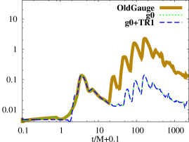
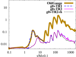
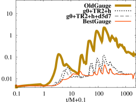
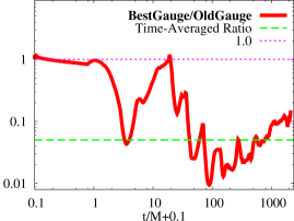
Figure 5: Excised L2 norm of Hamiltonian constraint violation vs time, $||\mathcal{H}||(t)$ (Eq. 18), as new techniques are added one-by-one at fixed “lr” resolution. Cases are as defined in Table 1. Upper-left panel: $||\mathcal{H}||(t)$ for cases OldGauge (thick brown), g0 (green dotted), and g0+TR1 (blue dashed). Upper-right panel: $||\mathcal{H}||(t)$ for cases OldGauge (thick brown), g0+TR1 (blue dashed), g0+TR2 (magenta solid), g0+TR2+h (black dotted). Lower-left panel: $||\mathcal{H}||(t)$ for cases OldGauge (thick brown), g0+TR2+h (black dotted), g0+TR2+h+d5d7 (gray dashed), and BestGauge (g1+TR2+h+d5d7; orange solid). Lower-right panel: $||\mathcal{H}||(t)$ for the BestGauge case, divided by $||\mathcal{H}||(t)$ for the OldGauge case (solid red). This ratio is compared to its time-averaged value ($\approx 0.05$, green dashed) and unity (magenta dotted). Values below unity indicate an improvement (reduction in $||\mathcal{H}||(t)$).

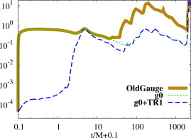
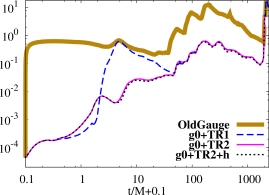
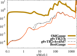
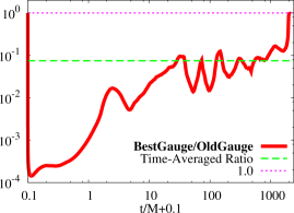
Figure 6: Excised L2 norm of $x$-component of Momentum constraint violation vs time, $||\mathcal{M}^{x}||(t)$ (Eq. 19), as new techniques are added one-by-one at fixed “lr” resolution. Cases are as defined in Table 1. Upper-left panel: $||\mathcal{M}^{x}||(t)$ for cases OldGauge (thick brown), g0 (green dotted), and g0+TR1 (blue dashed). Upper-right panel: $||\mathcal{M}^{x}||(t)$ for cases OldGauge (thick brown), g0+TR1 (blue dashed), g0+TR2 (magenta solid), g0+TR2+h (black dotted). Lower-left panel: $||\mathcal{M}^{x}||(t)$ for cases OldGauge (thick brown), g0+TR2+h (black dotted), g0+TR2+h+d5d7 (gray dashed), and BestGauge (g1+TR2+h+d5d7; orange solid). Lower-right panel: $||\mathcal{M}^{x}||(t)$ for the BestGauge case, divided by $||\mathcal{M}^{x}||(t)$ for the OldGauge case (solid red). This ratio is compared to its time-averaged value ($\approx 0.075$, green dashed) and unity (magenta dotted). Values below unity indicate an improvement (reduction in $||\mathcal{M}^{x}||(t)$).

IV.2 Noise Reduction Features of New Gauge Conditions

In addition to constraint-violation reductions, our new gauge conditions also act to reduce short-wavelength noise in the GWs ($\psi^{4}(t)$) as well as the surface-integral representations of ADM mass and angular momentum. We present these improvements here.

IV.2.1 Reduction of Noise in $\psi^{4}_{2,2}$

The left panel of Fig. 7 shows how short-period noise in $\psi^{4}_{2,2}(t-r)$ is significantly reduced when we choose a gauge in which the lapse speed is accelerated radially outward (g0), keeping all else identical to a standard moving-puncture gauge choice (OldGauge). Notice that the characteristic period for this noise is $P\sim 10M$, which is made clear in the right panel, which plots the power spectra of Re($\psi^{4}_{2,2}(t)$) for cases OldGauge, g0, and BestGauge (g1+TR2+h+d5d7) during early inspiral ($50\lesssim(t-r)/M\lesssim 1160$), when the signal-to-noise ratio of our numerical waveforms after junk radiation is lowest. Notice that accelerating the outgoing lapse wave speed has the largest impact on reducing high-frequency noise in Re($\psi^{4}_{2,2}(t)$), diminishing the noise by nearly an order of magnitude at the peak noise frequency (period of $\approx 10M$). Also, although additional tricks have some noticeable impact on constraint violations, they appear to contribute only a small amount to waveform noise at the shortest wavelengths.

Although we concentrate here on the dominant, ($l,m$)=(2,2), mode, we find significant noise reduction in sub-dominant modes as well. As an example, Fig. 8 demonstrates that in OldGauge, the amplitude of the ($l,m$)=(4,4) mode of $\psi^{4}$ is dominated by noise throughout a significant fraction of the inspiral. However, in BestGauge the noise is mostly non-dominant. Based on this and observations of other non-dominant modes, we conclude that these gauge improvements stand to improve the usefulness of sub-dominant modes from BSSN/MP evolutions.

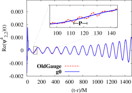
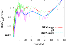
Figure 7: Inspiral waveform noise analysis. Left panel: Re($\psi^{4}_{2,2}$) versus retarded time, for cases OldGauge (dashed red) and g0 (solid blue). Inset magnifies noisiest part of waveform, demonstrating that the dominant noise frequency corresponds to a wave period of $P\approx 10M$ in the OldGauge case. Right panel: Power spectrum of Re($\psi^{4}_{2,2}$) versus wave period during inspiral, including data from $(t-r)/M\approx 58$ to $1160$, for cases OldGauge (thin green line: raw data, thick dashed red line: Bézier-smoothed data; i.e., fit to a degree-$n$ Bézier curve for $n$ data points), g0 (thin magenta line: raw data, thick solid blue line: Bézier-smoothed data), and BestGauge (g1+TR2+h+d5d7; thick dot-dashed cyan line: Bézier-smoothed data). All data plotted in this figure are from “lr” resolution runs, and Re($\psi^{4}_{2,2}$) data are from extraction radius $r=68.6M$. Re($\psi^{4}_{2,2}$) time series data were multiplied by the tapering function $\operatorname{Erf}(t;200,50)\times\operatorname{Erf}(-t;-1300,150)$ prior to the Fourier transform, to smoothly suppress junk radiation before $\sim 100M$ and the high-frequency late-inspiral/merger signals after $\sim 1500M$.

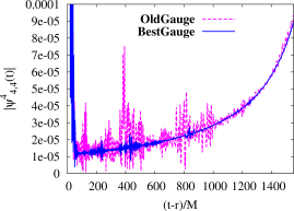
Figure 8: Amplitude of $\psi^{4}_{4,4}$ versus retarded time at “hhr” resolution, for cases OldGauge (dashed magenta) and BestGauge (solid blue).

IV.2.2 Reduction of Noise in ADM Surface Integrals

It has been found that surface integral representations of ADM mass $M(t)$ and angular momentum $J(t)$ (Eqs. 20 and 21) are noisy and suffer from large drifts in AMR moving-puncture BBH evolutions Marronetti et al. (2007). Though getting around the problem is usually a matter of recasting the distant surface integral into a sum of surface plus volume integrals, we find that this may be unnecessary with suitable gauge improvements. Figure 9 plots $M(t)$ and $J(t)$ surface integrals as measured at $r=114.2M$, comparing our original moving-puncture gauge choice (OldGauge) with our most sophisticated modification, g1+TR2+h+d5d7 (BestGauge), all at “hhr” resolution. The overall pattern is a drop in $M(t)$ and $J(t)$ as the GWs pass through the surface integral radius. However, our new gauge choices reduce noise in these surface integral diagnostics by a huge factor during inspiral, particularly $J(t)$. This demonstrates that noise in the region far from the BHs is not restricted to GWs, at least throughout the inspiral. However, after merger a large amount of noise in $J(t)$ remains, despite our gauge improvements.

We believe the lack of noise reduction in $J(t)$ at late times may be related to the spike in momentum constraint violation observed at roughly the same (retarded) time (see Sec. IV.1.1), which we hypothesized may have something to do with either the rapid settling of the gauge or the outgoing short-wavelength physical waves at and after merger.

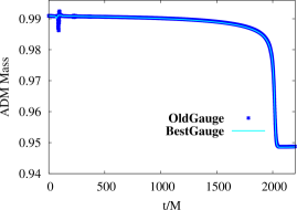
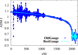
Figure 9: ADM surface integral noise analysis. Left panel: ADM mass $M(t)$ (Eq. 20), as measured by a surface integral at $r=114.2M$. Large blue points denote OldGauge case and thin cyan line BestGauge (g1+TR2+h+d5d7). Note that all data are taken from the “hhr” resolution runs. Right panel: Same as left plot, except ADM angular momentum $J(t)$ (Eq. 21) is plotted.

IV.3 Convergence Study

In a mixed-order finite-difference code such as ours, in which some components converge at different orders, we must be particularly careful about error estimates, as lower-order errors can sometimes be non-dominant, leading to higher-order convergence than otherwise expected. In such a scheme, numerical results for a quantity $Q_{\text{numerical}}$ at a given gridpoint, time, and grid spacing $\Delta x$, are related to the exact quantity $Q_{\text{exact}}$, via the following equation

$$Q_{\text{numerical}}(\Delta x)=Q_{\text{exact}}+C\Delta x^{n}+\mathcal{O}(\Delta x^{m})$$ (22)

where $C$ is a constant, $n$ is the dominant convergence order, $m\neq n$ is the next dominant convergence order, and $m<n$ is possible. Generally we would aim to have $C\Delta x^{n}\gg\mathcal{O}(\Delta x^{m})$, so the $\mathcal{O}(\Delta x^{m})$ term can be neglected. When non-dominant convergence order terms are neglected in this way, we call $Q_{\text{exact}}$ the Richardson-extrapolated $Q$, $Q_{\text{RE}}$, as it provides an estimate for $Q$ that removes the dominant error term, similar to Richardson (1911):

$$Q_{\text{RE}}=Q_{\text{numerical}}(\Delta x)-C\Delta x^{n}.$$ (23)

AMR prolongations in time and space are performed with second- and fifth-order-accurate stencils, respectively, and temporal and spatial derivatives via fourth- and sixth-order-accurate finite-difference stencils, respectively. Thus the dominant convergence order $n$ is a priori unknown in our BBH calculations, as they are of mixed order. As described in Sec. III.2, we have reduced the timestep on all grids well below the CFL limit to prevent the relatively low-order temporal differencing and interpolations from dominating our errors.

To determine the dominant convergence order $n$, we perform runs at three resolutions, obtaining three values for $Q_{\text{numerical}}(\Delta x)$. With these three knowns, we then employ a bisection technique to solve Eq. (23) for unknowns $n$, $Q_{\text{RE}}$ and $C$.

For quantities $Q_{\text{numerical}}(\Delta x)$ that are also functions of time (e.g., $\psi^{4}(t)$), we obtain estimates for $n$ each time $Q_{\text{numerical}}(\Delta x)$ is output by the code. We then define the dominant convergence order as the average of all bisection-calculated estimates for $n$, rounded to the nearest integer. This averaged, rounded value for $n$, combined with $Q_{\text{numerical}}(\Delta x)$ at the two lowest resolutions of the three used to obtain $n$, are chosen as inputs to solve the linear $2\times 2$ system for $C$ and $Q_{\text{RE}}$. We then find another estimate for $Q_{\text{RE}}$ combining the same value for $n$ with the two highest resolutions of the three $Q_{\text{numerical}}(\Delta x)$ used to estimate $n$. The difference between these two values for $Q_{\text{RE}}$ is used as an error estimate, as deviations from zero will be caused by variations in $n$ as well as higher-order terms (cf. Eqs. (23) and (22)).

In the special case where $Q_{\text{RE}}\to 0$, as is expected for quantities that should converge to zero (e.g., constraint violations), we may solve Eq. (23) for $n$ with only two realizations of $Q_{\text{numerical}}(\Delta x)$. In this special case, $n$ can be found analytically.

IV.3.1 Irreducible Mass Convergence

Figure 10 presents a convergence study of $M_{\text{irr}}(t)$ for the spinning BH (i.e., the BH with initial spin parameter$=0.3$) at various resolutions. For ease of comparison (it is difficult to distinguish a dotted line from a dashed one if data are exceedingly noisy), the “mr”, “hr”, and “hhr” data are Bézier-smoothed (i.e., fit to a degree-$n$ Bézier curve for $n$ data points). However, to show how the high-frequency noise in $M_{\text{irr}}(t)$ is affected by gauge choice, we do not smooth the “lr” run data. Notice how $M_{\text{irr}}(t)$ data are significantly less noisy in the improved gauge case BestGauge (right panel) than in the OldGauge case (left panel), demonstrating that gauge-generated noise affects the strong-field region as well. We observe the same relative noise in the higher-resolution runs prior to smoothing. We also note that our gauge improvements have little impact on the secular drift in $M_{\text{irr}}(t)$. As for the initially nonspinning BH, similar results are observed, except the “lr” run is not as much an outlier.

To understand why the “lr” resolution run appears to be such a significant outlier, we take a look at the isolated horizon formalism spin Ashtekar and Krishnan (2004) of the initially spinning BH, shown in Fig. 11. Notice the secular increase in dimensionless spin parameter $(J/M^{2})_{\text{IHF}}$ at “lr” resolution, which completely dwarfs spin parameter drifts in the highest three resolution runs. Figure 11 shows data from the OldGauge case only. For comparison, we report that at “lr” resolution, g0+TR2+h shares the same drift as OldGauge to within a percent, and g1+TR2+h+d5d7 (BestGauge) exhibits about 6% less drift. Finally we note that for the initially nonspinning BH, we observe no significant drift in spin parameter over time. Based on these observations, we conclude that the “lr” run is at insufficient resolution to properly resolve the spinning BH.

Throwing out data at the “lr” resolution, and using data at resolutions {mr,hr,hhr}, Fig. 12 shows convergence order $n$ for $M_{\text{irr}}$ (Eq. 23) versus time. This panel compares observed convergence order $n$ for both BHs in all three cases throughout much of the inspiral. Convergence is poor for $t\gtrsim 1100M$, as BH2 $M_{\text{irr}}$ data at all three resolutions cross near $t\approx 1300M$, regardless of gauge choice. Apparently this clear non-convergence in BH2 negatively impacts BH1 convergence as well. Outside of this non-convergent episode, we find average convergence orders slightly higher than fifth order (our chosen spatial prolongation order), independent of the gauge choice, although the results using the BestGauge choice are clearly less noisy.

In the next section, we show that this nonconvergence in irreducible mass drift at low resolution does not translate to nonconvergence at low resolution in constraint violations.

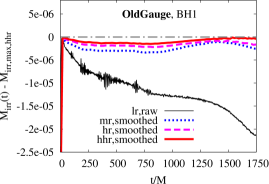
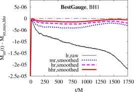
Figure 10: Convergence study: $M_{\text{irr}}(t)$. Left panel: $M_{\text{irr}}(t)-M_{\text{irr,hhr,max}}$ over time for BH1 (i.e., the BH with initial spin parameter$=0.3$), where $M_{\text{irr,hhr,max}}$ is the maximum value of $M_{\text{irr}}$ in the “hhr” run. This panel plots data for the OldGauge case at resolutions “lr” (solid red), “mr” (medium-dashed blue), “hr” (long-dashed magenta), and “hhr” (dotted green). Right panel: Same as left panel, but for case BestGauge (g1+TR2+h+d5d7). “smoothed” denotes that the $n$ data points for a given dataset plotted in this figure have been fit to degree-$n$ Bézier curve, and the resulting Bézier curve is shown.

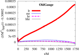
Figure 11: Spin parameter versus time for BH1 (i.e., “the spinning BH”, with initial spin parameter $\approx 0.3$), as given by isolated horizon formalism. Data are plotted at resolutions “lr” (thick solid red), “mr” (dotted blue), “hr” (dashed magenta), and “hhr” (thin solid gray). Note that the offset 0.30002 is chosen for $(J/M^{2})_{\text{IHF}}(t)$, which is the value all runs converge to after a rapid initial settling. We attribute this settling to the fact that our initial data are conformally flat. Note also that only case OldGauge is shown, as all other cases share the same qualitative behavior.

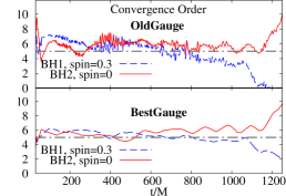
Figure 12: Convergence study: Implied convergence order $n$ (Eq. 23) for $M_{\text{irr}}(t)$, using $M_{\text{irr}}(t)$ data at three highest resolutions {mr,hr,hhr} for both BHs during inspiral. Convergence order for BH1 (initial spin parameter$=0.3$; solid red) and BH2 (initially nonspinning; dashed blue) are compared to $n=5$ (dot-dashed gray). The top plot shows data from the OldGauge case the middle plot g0+TR2+h, and the bottom BestGauge (g1+TR2+h+d5d7). For ease of analysis, all raw $M_{\text{irr}}(t)$ data in this plot were first smoothed with a moving-window linear least-squares algorithm prior to computing convergence order. Also, data in the range $t/M<30$ and $t/M>1250$ have been removed, as $M_{\text{irr}}(t)$ at all three resolutions overlaps at $t/M=0$ and $t/M\approx 1300$ in the nonspinning BH (BH2) data, so near these points convergence order estimates for BH2 are unreliable.

IV.3.2 Convergence to Zero of Constraint Violations

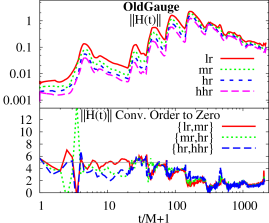
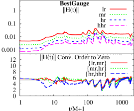
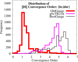
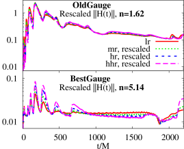
Figure 13: Convergence to zero of Hamiltonian constraint violations. Upper-left panel: Top plot shows raw $||\mathcal{H}(t)||$ at resolutions “lr” (solid red), “mr” (dotted green), “hr” (short-dashed blue), and “hhr” (long-dashed magenta) for OldGauge case. Bottom plot shows implied convergence order $n$ (Eq. 23) to zero for resolution pairs {lr,mr} (solid red); {mr,hr} (dotted green); and {hr,hhr} (dashed blue). Upper-right panel: Same as upper-left panel, except for BestGauge case (g1+TR2+h+d5d7). Lower-left panel: Distribution of $||\mathcal{H}(t)||$ convergence order, using {hr,hhr} data for OldGauge case (thick red), g0+TR2+h (medium thickness magenta), and BestGauge (g1+TR2+h+d5d7; thin black). Note that the thick red line corresponds to the distribution of convergence order, as shown by the red line in the bottom plot of the upper-left panel. Lower-right panel: Top plot: $||\mathcal{H}(t)||$ for OldGauge case, rescaled according to the observed average convergence order to zero over all resolutions, $n=1.62$. Bottom plot: same as top, except for BestGauge (g1+TR2+h+d5d7) case, where the average convergence order to zero over all resolutions is found to be $n=5.14$. All cases are rescaled to “lr” resolution.

Table 2: Convergence to zero of Hamiltonian and $x$-component of Momentum constraint violations. “Median” (“Mean”) numbers denote median (average) convergence order using an evenly-spaced sample of integrated L2-norm of constraint violations in time. This integral excludes regions around the BHs (Eq. 18), and for $||\mathcal{H}_{\text{inner}}||$, the region $r>32.3M$ as well. Note that for consistency, all data are truncated at time $t=2086.4M$, which is the earliest time at which a run was stopped ($\approx 210M$ after merger).

Case Name	$||\mathcal{H}||_{\text{lr,mr}}$ Median (Mean)	$||\mathcal{H}||_{\text{mr,hr}}$ Median (Mean)	$||\mathcal{H}||_{\text{hr,hhr}}$ Median (Mean)
OldGauge	1.43 (1.64)	1.30 (1.62)	1.46 (1.60)
g0+TR2+h	5.17 (4.70)	5.97 (4.31)	5.27 (4.24)
g0+TR2+h+d5d7	5.57 (5.27)	5.86 (4.97)	No hhr
BestGauge (g1+TR2+h+d5d7)	5.63 (5.38)	5.92 (5.16)	5.41 (4.87)
	$||\mathcal{H}_{\text{inner}}||_{\text{lr,mr}}$ Median (Mean)	$||\mathcal{H}_{\text{inner}}||_{\text{mr,hr}}$ Median (Mean)	$||\mathcal{H}_{\text{inner}}||_{\text{hr,hhr}}$ Median (Mean)
OldGauge	5.77 (5.75)	5.72 (5.46)	5.98 (5.87)
g0+TR2+h	5.82 (5.80)	5.86 (5.67)	5.96 (5.74)
g0+TR2+h+d5d7	5.78 (5.75)	5.61 (5.69)	No hhr
BestGauge (g1+TR2+h+d5d7)	5.81 (5.79)	5.94 (5.77)	5.76 (5.71)
	$||\mathcal{M}^{x}||_{\text{lr,mr}}$ Median (Mean)	$||\mathcal{M}^{x}||_{\text{mr,hr}}$ Median (Mean)	$||\mathcal{M}^{x}||_{\text{hr,hhr}}$ Median (Mean)
OldGauge	1.37 (1.81)	1.37 (1.62)	1.29 (1.96)
g0+TR2+h	1.09 (1.71)	1.00 (1.98)	1.37 (2.00)
g0+TR2+h+d5d7	1.27 (1.86)	1.31 (1.86)	No hhr
BestGauge (g1+TR2+h+d5d7)	1.24 (1.94)	1.26 (1.84)	1.78 (1.91)

Table 2 presents the average and median order at which Hamiltonian and ($x$-component) momentum constraints converge to zero for various cases. To better understand how these numbers are generated, Fig. 13 outlines the procedure. The top left (right) plots in the upper panels show the raw Hamiltonian constraint data $||\mathcal{H}(t)||$ (Eq. 18) for the OldGauge (BestGauge) case, and the bottom plots of the upper panels use data at pairs of resolutions to solve for the implied convergence order $n$ (Eq. 23, where $Q_{\text{RE}}\to 0$, leaving only $C$ and $n$ as unknowns). Using many data points for $n$, uniformly spaced in time, we can then construct histograms of convergence order from this plot. The lower-left panel shows the histogram of convergence order for “hr” and “hhr” resolutions, where the thick red line corresponds to the solid red curve in the bottom plot of the upper-left panel. This histogram is compared to the same histogram for cases g0+TR2+h and BestGauge (g1+TR2+h+d5d7). We point out two clear patterns: (1) the g0+TR2+h and BestGauge cases possess significantly higher average convergence order than OldGauge, (2) BestGauge appears to converge at a higher average convergence order than g0+TR2+h. Notice the distribution widens with increasing average convergence order. This is a reflection of the fact that after t 300M, the OldGauge ——H—— converges below second-order and remains there until merger. In BestGauge, convergence order drops significantly as the sharp lapse wave crosses progressively lower-resolution refinement boundaries. However, this subconvergent spike in noise does not translate to sub-convergence later on in the evolution. We attribute this to the lapse stretching and smoothing features of BestGauge. Instead of plotting histograms for all cases at all resolutions, we simply report the median and mean convergence orders for all cases for which multiple resolution data are available (Table 2).

According to Table 2, we expect $||\mathcal{H}(t)||$ to converge to zero on average at order $n=1.62$ in the OldGauge case, and $n=5.14$ in the BestGauge (g1+TR2+h+d5d7) case. The lower-right panel of Fig. 13 demonstrates how well data at different resolutions overlap when rescaled according to these observed mean convergence orders. Notice that although convergence order drops to as low as second order at each spike in the BestGauge $||\mathcal{H}(t)||$ (cf. upper-right and lower-right panels), BestGauge convergence order equilibrates at late times to $n\approx 6$. In the OldGauge case, $||\mathcal{H}(t)||$ convergence order steadily drops from the outset of the calculation (upper-left panel) as the initial sharp lapse wave crosses into progressively lower resolution AMR grid boundaries.

Recall that in Fig. 5, we found that $||\mathcal{H}(t)||$ is reduced by a factor of 20 on average in the BestGauge case, compared to a standard moving-puncture gauge choice (OldGauge). Table 2 demonstrates that the convergence order in $||\mathcal{H}(t)||$ is also significantly improved with our gauge improvements, increasing from below second-order to nearly sixth-order convergence. Thus at higher resolutions, we expect our gauge improvements to reduce $||\mathcal{H}(t)||$ by an even higher factor than that observed at “lr” resolution. In fact “BestGauge, hhr” drops $||\mathcal{H}(t)||$ by a factor of approximately 58, as compared to the “OldGauge, hhr” case.

When the L2 norm of $\mathcal{H}(t)$ (Eq. 18) excises the region outside $r=32.3M$ (i.e., $||\mathcal{H}_{\text{inner}}||$ in Table 2), we observe nearly sixth-order convergence in all cases. Thus a bulk of sub-convergent Hamiltonian constraint violations comes from the outer regions, where gravitational waves are measured, and the under-resolution of the spinning BH at “lr” resolution (as discussed in Sec. IV.3.1) does not appear to translate to inconsistent convergence at low resolutions in constraint violations.

We did not have such an “inner region” diagnostic for momentum constraint violations (i.e., an $||\mathcal{M}^{x}_{\text{inner}}||$ diagnostic). Recall that at “lr” resolution, $||\mathcal{M}^{x}||$ has been reduced on average by a factor of $\approx 13.4$ with our new gauge choices (Fig. 6). However, its convergence to zero does not improve significantly and remains between first and second-order regardless of gauge choice. This may be due to the fact that even in our most advanced gauge choice (BestGauge), some high-frequency noise remains and further efforts may be required to tamp down this remaining noise.

So do drastic constraint violation reductions in the outer regions of our grid translate to improvements in gravitational waveform (i.e., $\psi^{4}$) convergence, or does the relatively large drift in the spinning BH’s spin parameter over time imply poor waveform convergence at “lr” resolution? The next section examines this question in detail.

IV.3.3 Waveform Convergence

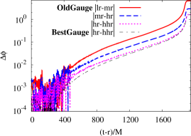
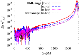
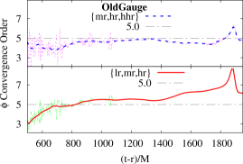
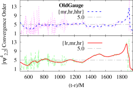
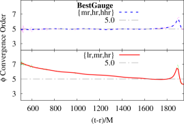
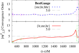
Figure 14: $\psi^{4}_{2,2}$ convergence study, using smoothed amplitude and phase data. Upper-left (right) panel: phase (amplitude) difference between pairs of resolutions, for OldGauge $|$lr-mr$|$ (thick solid red), $|$mr-hr$|$ (thick dashed blue), and $|$hr-hhr$|$ (thick dotted magenta), as well as BestGauge $|$hr-hhr$|$ (g1+TR2+h+d5d7, thin dashed black). Middle-left (right) panel: OldGauge phase (amplitude) convergence order versus time, using results from {lr,mr,hr} resolutions (raw data: thin dashed green, Bézier-smoothed data: thick solid red) and {mr,hr,hhr} resolutions (raw data: thin dashed magenta, Bézier-smoothed data: thick dashed blue). Lower-left (right) panel: same as middle panels, except for BestGauge (g1+TR2+h+d5d7). Please note that for ease of analysis, all raw amplitude and phase data in this figure were first smoothed with a moving-window quadratic least-squares fit method prior to computing convergence order, and where specified, Bézier smoothing was applied separately to the resulting convergence order data as well. Also, data $(t-r)/M<500$ have been removed from convergence order plots, as they are too noisy even after smoothing to show a clear convergence order (see top panels). $\psi^{4}_{2,2}$ data are measured at radius $r=68.6M$.

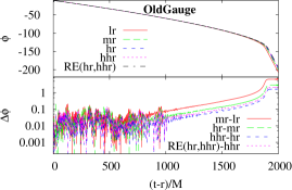
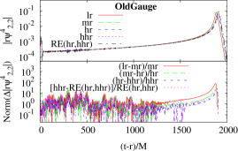
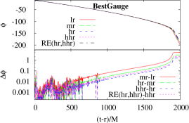
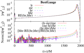
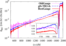
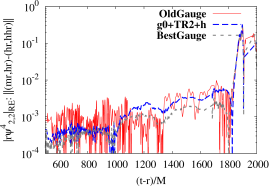
Figure 15: $\psi^{4}_{2,2}$ convergence and error-analysis study, using raw, unsmoothed phase and amplitude data. Top panels: Upper-left (right) plot: Phase (Amplitude) versus retarded time, for OldGauge case at resolutions “lr” (solid red), “mr” (long-dashed green), “hr” (medium-dashed blue), and “hhr” (dotted magenta). Richardson-extrapolated phase is overlaid, using data from “hr” and “hhr” resolutions, and assuming constant fifth-order convergence (dash-dotted black). Lower-left (right) plot: simple (not absolute value of) difference in phase (normalized amplitude) between resolutions. Middle panels: same as top panels, but for case BestGauge (g1+TR2+h+d5d7). Bottom panels: left (right) plot shows $|$RE(mr,hr)-RE(hr,hhr)$|$ for waveform phase (amplitude) versus retarded time, assuming fifth-order convergence, where RE(mr,hr) denotes the Richardson-extrapolated value combining phase (amplitude) numerical data at resolutions {mr,hr} with the assumption of fixed $n=5$ convergence order (Eq. 23). Amplitude data are normalized by the higher-resolution value. Cases OldGauge (dotted magenta), g0+TR2+h (long-dashed blue), and BestGauge (g1+TR2+h+d5d7; solid red) are compared. Zoom inset on the left plot shows accumulated phase difference near the end of the inspiral, with vertical gray line denoting $M\omega_{2,2}=0.2$ (corresponding to a retarded time of $(t-r)/M\approx 1866$). All $\psi^{4}_{2,2}$ data are measured at radius $r=68.6M$.

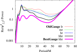
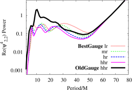
Figure 16: Re($\psi^{4}_{2,2}$) noise convergence properties, during early inspiral [$58\lesssim(t-r)/M\lesssim 1160$]. Left panel: Bézier-smoothed Power spectra of Re($\psi^{4}_{2,2}$) for case OldGauge, at resolutions “lr” (dotted red), “mr” (short-dashed green), “hr” (dashed blue), and “hhr” (solid black). These are compared to the same quantity at “hhr” resolution for case BestGauge (g1+TR2+h+d5d7; thick magenta). Right panel: Bézier-smoothed power spectra of Re($\psi^{4}_{2,2}$) for case BestGauge, at resolutions “lr” (dotted red), “mr” (short-dashed green), “hr” (dashed blue), and “hhr” (solid magenta). These are compared to the same quantity at “hhr” resolution for case OldGauge (thick black). Note that all Re($\psi^{4}_{2,2}$) data plotted are measured at radius $r=68.6M$, and for an example of unsmoothed data, see Fig. 7. Re($\psi^{4}_{2,2}$) time series data were multiplied by the tapering function $\operatorname{Erf}(t;200,50)\times\operatorname{Erf}(-t;-1300,150)$ prior to the Fourier transform.

Figure 14 presents a gravitational waveform convergence study, separating $\psi^{4}_{2,2}(t)$ into amplitude and phase separately, as these quantities could be influenced differently by truncation error Husa et al. (2008).

The top left (right) panel of Fig. 14 shows $|Q_{\text{numerical}}(\Delta x_{1})-Q_{\text{numerical}}(\Delta x_{2})|$, where $Q$ is the smoothed phase (amplitude) of $\psi^{4}_{2,2}(t)$, and {$\Delta x_{1},\Delta x_{2}$} denotes data at two adjacent resolutions in the set {lr,mr,hr,hhr}. Notice that the {hr,hhr} phase difference is slightly smaller during inspiral in the BestGauge (g1+TR2+h+d5d7) than the OldGauge case. This is one measure that demonstrates our gauge improvements reduce phase errors.

The remaining left (right) panels of Fig. 14 plot convergence order $n$ in $\psi^{4}_{2,2}$ phase (amplitude) as a function of time, comparing the OldGauge (middle panels) to the BestGauge (g1+TR2+h+d5d7; bottom panels) cases. At the three lowest resolutions {lr,mr,hr}, inconsistent convergence between amplitude and phase is observed, regardless of gauge choice. We attribute this to the under-resolution of the spinning BH (Sec. IV.3.1). Cleaner convergence is observed when computing $n$ from data at the three highest resolutions {mr,hr,hhr}. However, convergence order in the OldGauge case oscillates significantly between $n=4$ and $n=5$ until $t\approx 1300M$, and then drops to $n\approx 4$ until merger. The same data from our BestGauge case indicate extremely steady $n=5$ convergence order with almost no oscillation, until merger.

At merger ($t\gtrsim 1750M$), loss in convergence is observed regardless of gauge choice, pointing to a non-convergent effect not addressed by our gauge modifications. However, there is some chance that this loss of convergence may be restored with another careful time reparameterization near merger, which will allow the gauge to more quickly settle as the gravitational fields undergo the extremely rapid changes associated with merger.

The consistent $n=5$ convergence observed in BestGauge is a highly significant result, as it strongly indicates that our errors are dominated by the fifth-order-accurate spatial interpolation errors at grid refinement boundaries in BestGauge. We could have reasonably expected this a priori given that the lower-order temporal errors have been tamped down significantly by our choice of timesteps well below the CFL limit. The convergence order oscillations in OldGauge below $n=5$ are troubling, leading us to question the reliability of Richardson-extrapolated estimates of $\psi^{4}_{2,2}$ that assume a standard, fixed-in-time integer convergence order when choosing OldGauge-like gauge conditions.

We believe that the OldGauge convergence order oscillations in $\psi^{4}_{2,2}$ amplitude and phase may be related to the large amount of power in $\psi^{4}_{2,2}$ noise, particularly at wave periods of $P\sim 10M$ as shown in Fig. 7, as this noise has been largely removed in the BestGauge case. In fact, in Sec. IV.3.4 below, we show that waveform noise at the dominant noise frequency ($P\approx 10M$) in OldGauge does not diminish with increasing resolution, at the resolutions chosen.

We end our discussion on Fig. 14 by cautioning that our clean, fifth-order convergence in BestGauge has only been demonstrated with the three highest resolutions, and that higher-resolution studies will be useful in cementing our conclusions. Although our gauge improvements have apparently eliminated the non-convergent gravitational waveform noise (as shown in Sec. IV.3.4 below), some noise does remain, and we anticipate that at high resolutions far beyond that attempted here, further gauge improvements may be necessary to maintain a uniform, integer convergence order.

We now turn our attention to the Richardson-extrapolated waveforms. Given that our gauge improvements yield cleaner gravitational-waveform convergence at higher resolutions, we may be able to more precisely estimate the true value of $\psi^{4}_{2,2}$ through Richardson extrapolation. The Richardson-extrapolated value is given by $Q_{\text{RE}}$ in Eq. (23), replacing $Q$ with $\psi^{4}_{2,2}$ at all times $t$. Since we have established the dominant waveform convergence order is cleanly $n=5$ for {mr,hr,hhr} resolutions, we can compute $\psi^{4}_{2,2,\text{RE}}$ in Eq. (23) by setting $n=5$ and combining numerical data at two resolutions.

The top and middle panels of Fig. 15 compare raw $\psi^{4}_{2,2}$ amplitude and phase data at all four resolutions to Richardson-extrapolated values at the highest two resolutions {hr,hhr}. At $t\lesssim 800M$ ($t\lesssim 1200M$) in the OldGauge (BestGauge), simple differences between data at adjacent resolutions are too noisy to easily distinguish convergence properties (top panels). This can be somewhat mitigated by careful smoothing, as was shown in Fig. 14, but both phase and amplitude data at $t\lesssim 500$ are too noisy to determine convergence order cleanly in OldGauge, even with smoothing. Due to the large noise reductions of BestGauge, the situation is greatly improved (middle panels), though determining convergence order in phase (amplitude) remains difficult for times $t\lesssim 600M$ ($t\lesssim 900M$) without smoothing. Notice that the difference between Richardson-extrapolated phase and amplitude data (as computed at {hr,hhr} resolutions) and “hhr” resolution data is larger than the difference between “hr” and “hhr” data.

The bottom left (right) panel of Fig. 15 shows differences in Richardson-extrapolated phase (amplitude) versus time. One Richardson-extrapolated value combines data at {mr,hr} resolutions—which we denote RE(mr,hr)—and the other combines {hr,hhr}—denoted by RE(hr,hhr). Any nonzero value for $|$RE(mr,hr)-RE(hr,hhr)$|$ may be caused by either deviations from fifth-order convergence—which we have shown to be particularly significant in OldGauge (Fig. 14)—or truncation errors at non-dominant orders (cf. Eqs. 23 and 22). Thus we consider $|$RE(mr,hr)-RE(hr,hhr)$|$ as an error estimate for phase, and $|$RE(mr,hr)-RE(hr,hhr)$|$/RE(hr,hhr) for amplitude.

Implied phase errors $|$RE(mr,hr)-RE(hr,hhr)$|$ increase with time, but far more smoothly in the improved gauge cases, as compared to the OldGauge case. Though phase errors are roughly comparable in the OldGauge and g0+TR2+h cases, we find a reduction in phase error of about $40\%$ in the BestGauge (g1+TR2+h+d5d7) case throughout inspiral and near merger. Normalized amplitude errors are much noisier, but appear about 40–50% smaller during inspiral in the BestGauge case as well, as compared to the OldGauge and g0+TR2+h cases. However, during and after merger, amplitude and phase errors for all three cases are large and overlap. These large errors are expected, as the BBH merger time changes as resolution is increased, and we do not account for this effect by, e.g., shifting the waveforms so that their merger times overlap.

We may use the two highest-resolution estimates for $\psi^{4}_{2,2,\text{RE}}$ to compute accumulated amplitude and phase errors at the end of inspiral, where we define the “end of inspiral” to be at the time in which gravitational wave frequency is $M\omega=0.2$. An almost identical frequency was used in the NINJA Ajith et al. (2012); Aasi et al. (2014) and NRAR Hinder et al. (2013) collaborations as the fiducial time at which to measure waveform amplitude and phase errors, the only difference being that we choose to normalize $\omega$ by total initial ADM mass instead of the combined initial masses of the punctures. The difference in frequency is less than one percent for runs presented here. We find accumulated phase errors at $M\omega=0.2$ (vertical line in inset) of approximately 0.046, 0.081, and 0.025 radians for OldGauge, g0+TR2+h, and BestGauge cases, respectively. Thus the BestGauge gauge choice reduces phase errors by about a factor of two. This is a rather unfortunate time to measure phase error, as the OldGauge case phase error does not increase as predictably as the BestGauge case, and just happens to experience a local minimum in the rate of phase error increase at $M\omega=0.2$. Had we measured phase errors slightly earlier or perhaps at a higher resolution, we might have seen further reduction of phase errors by BestGauge.

As pointed out earlier, normalized amplitude errors near merger are comparable between the different cases, and we measure them at the “end of inspiral” to be 5.7%, 6.0%, and 5.8% for OldGauge, g0+TR2+h, and BestGauge cases, respectively. We conclude that although amplitude errors are clearly smaller during inspiral in the BestGauge case, they are comparable just prior to merger.

In Sec. IV.2, we established that, when compared to the OldGauge case, the BestGauge case significantly reduces noise in gravitational waveforms, particularly at peak noise frequencies. Further, we showed in the previous section that GWs produced by BestGauge are very consistently fifth-order convergent, while the OldGauge case experiences disturbing oscillations in implied convergence order. We suspect that these convergence order oscillations are related to the much noisier waveforms in OldGauge, but we would naïvely expect that the noise should reduce with increasing resolution. The next section demonstrates that at peak noise frequencies, the noise in OldGauge does not diminish with increasing resolution.

IV.3.4 Waveform Noise Convergence Properties

Figure 16 presents a power spectrum analysis of waveform noise convergence. The left panel shows that the largest noise-related spike in OldGauge Re($\psi^{4}_{2,2}$) power does not appear to diminish with increased resolution, lending support to the notion that poor waveform convergence in OldGauge is due to high-frequency noise. In fact, we find that the power attributable to noise in OldGauge at $P\approx 10M$ is about 1% of the maximum power, corresponding to the physical GW signal (at GW periods of half the binary orbital period). Next notice that this large, non-converging noise-related spike in the power spectrum in OldGauge runs has been reduced by about an order of magnitude in our BestGauge gauge choice. This is consistent with the time-domain data of Fig. 7, in which waveform noise at “lr” resolution is shown to be hugely reduced in the BestGauge case, as compared to OldGauge. In BestGauge, we observe three distinct bumps in the power spectrum, likely associated with noise. Unlike the dominant noise-related spike at $P\approx 10M$ in OldGauge, these three bumps in the BestGauge power spectra appear to drop more cleanly with increasing resolution than OldGauge, and as resolution is increased, the bumps appear to decrease in amplitude and shift toward shorter wave periods.

V Conclusions and Future Work

It has been found that the standard BSSN/MP+AMR paradigm yields inconsistent convergence in gravitational waveforms in BBH evolutions. Without consistent convergence, it may be impossible to produce reliable error estimates for these waveforms, particularly when very high accuracies are needed. It has been hypothesized Zlochower et al. (2012) that this inconsistent convergence may be related to short-wavelength waves being reflected from grid-refinement boundaries, producing high-frequency noise and constraint violations.

We present a set of improvements to the moving-puncture gauge conditions that, with negligible increase in computational expense, greatly reduce noise and improve convergence properties of gravitational waveforms from BBH inspiral and mergers. These improvements are presented in the context of an NRAR Hinder et al. (2013) BBH calculation that evolves a low-eccentricity BBH system $\approx 11$ orbits to merger, where one BH has an initial dimensionless spin of $0.3$ aligned with the orbital angular momentum, and the other is nonspinning. Evolutions are performed at up to four resolutions with a variety of gauge choices, starting with the “standard” moving puncture gauge choice and adding improvements one by one until our “best” gauge choice is reached.

Our gauge improvements in part stem from the observation that regularly-spaced spikes in Hamiltonian constraint violations are timed precisely to the grid-refinement boundary crossings of an early outgoing wave traveling at coordinate speed $\sqrt{2}$. Based on linear analyses Alcubierre (2003), we know of only one propagation mode with that speed in the standard BSSN/MP formulation, which primarily involves the lapse and is governed by the lapse evolution gauge condition.

The initial outgoing lapse wave pulse possesses sharp features, which are problematic because, as Zlochower et al. (2012) points out, high-frequency waves crossing into a coarser AMR grid will be partially reflected at the boundary, generating noise. Now the lapse and its derivatives are strongly coupled to the gravitational field evolution equations, so noise generated by this sharp outgoing lapse pulse crossing refinement boundaries can be easily converted to noise in gravitational field variables (such as GWs) and constraint-violating modes (cf. Etienne et al. (2012)).

Guided by this, we focus our efforts primarily on modifications to the lapse evolution equation, aimed at stretching and smoothing the initial outgoing lapse wave pulse. We stretch the lapse wave by monotonically increasing its speed as it propagates outward so that the front of the lapse pulse propagates slightly faster than the back. We smooth the lapse wave by adding both parabolic and stronger-than-usual Kreiss-Oliger dissipation terms. The most significant improvements spawn from the stretching of the initial lapse pulse.

Despite the stretching of the initial lapse pulse, early-time spikes in the constraint violations are not reduced. We are able to significantly tamp down these spikes via a time reparameterization that greatly accelerates the initial evolution of the lapse and shift relative to the BSSN gravitational field evolution variables. Effectively, this modification makes lapse waves propagate at speeds up to $\sim 30$ times the coordinate speed of light initially, enabling the lapse to respond much more quickly to the rapidly-settling gravitational fields in the strong-field region during the early evolution.

Our “best” gauge condition (BestGauge) reduces Hamiltonian and momentum constraint violations by factors of $\sim 20$ and $\sim 13$, respectively. In addition, with this same gauge choice, noise in the dominant gravitational-wave mode—$\psi^{4}_{2,2}(t)$—is reduced by nearly an order of magnitude, particularly at peak noise frequencies. Such numerical noise can be far more problematic in sub-dominant [i.e., $(l,m)\neq$(2,2)] modes, at times completely obscuring the signal. As an example, with OldGauge, the $(l,m)$=(4,4) mode is noise-dominated throughout much of the inspiral, but with the new gauge improvements, this mode is much cleaner and more amenable to analysis. We observe improvements, generally of a lesser degree, in other sub-dominant modes as well.

Finally, we observe a significant reduction in ADM mass and angular momentum noise at large radius, particularly during inspiral and merger. Regardless of gauge choice, we observe a large amount of noise in ADM angular momentum just after merger, corresponding to a spike in momentum constraint at about this time. We are uncertain of the cause for this noise/spike, but suspect they may be due to either rapid coordinate and spacetime evolution associated with BH merger, or possibly high-frequency physical waves propagating outward into less-refined numerical grids. This warrants further investigation, as the former hypothesis can be tested through a late-time time reparameterization and the latter through grid structure adjustments.

In addition to analyses of how constraint violations and noise are affected by our new gauge choices, we perform a suite of constraint-violation, irreducible-mass, and waveform ($\psi^{4}_{2,2}$) convergence tests with a set of three gauge choices, starting from the “standard” moving-puncture gauge choice (OldGauge) to our “best” gauge choice (BestGauge).

Using the “standard” moving-puncture gauge choice (OldGauge), the L2 norm of Hamiltonian constraint violations converges to zero at between first and second order with increasing resolution. If this L2 norm integral excludes the wavezone region far from the binary, convergence order increases to between fifth and sixth order, indicating that subconvergence is related to effects far from the binary, on distant, low-resolution grids. Meanwhile, with our improved gauge choices, we observe between fifth- and sixth-order convergence in this diagnostic even when the integral extends to the outer boundary. Though momentum constraint violations at a given resolution are significantly reduced with our new gauge choices, we do not observe an improvement in the convergence to zero of momentum constraint violations. This may be due to the fact that even in our “best” gauge choice, some high-frequency noise remains in our BBH calculations.

Based on our waveform convergence analyses, we find that $\psi^{4}_{2,2}(t)$ data at {mr,hr,hhr} resolutions yield approximate fifth-order convergence, though large fluctuations around fifth order are observed in the OldGauge case. These fluctuations are significantly reduced when improved gauge conditions are adopted, particularly in the BestGauge case.

With such consistent fifth-order convergence observed in the highest three resolutions in our best gauge choice (BestGauge), we then analyze the difference between two Richardson-extrapolated realizations of phase and normalized amplitude. One realization uses data at “hr” and “hhr” resolutions and the other “mr” and “hr” resolutions. Any nonzero difference between these Richardson-extrapolated realizations of phase and normalized amplitude can be attributed to fluctuations in assumed convergence order $n$ from $n=5$ (which appears to be related to noise) or to error from higher-order terms (cf. Eqs. 23 and 22). Since these differences in Richardson-extrapolated values are directly related to errors, we use them as our error estimates for the amplitude and phase (though it may be an unconventional choice; cf. Hinder et al. (2013)). Comparing the “standard” moving-puncture gauge choice to our “best” gauge, we find significant (factor of $\sim$ 2) reductions in both amplitude and phase errors during inspiral. At the end of the inspiral, when the frequency of the $\psi^{4}_{2,2}$ is $M\omega=0.2$, we observe roughly a factor of two reduction in phase errors in the BestGauge case but no significant improvement in amplitude errors, as these are dominated near merger by small offsets in the time of merger at different resolutions.

We then perform a GW noise analysis, comparing OldGauge and BestGauge results at different resolutions (see Fig. 16). In the OldGauge case, the largest spike in GW power directly related to numerical GW noise, at wave periods $P\approx 10M$ (Fig. 7), does not drop with increasing resolution. Further, we find that the noise-dominated power in this OldGauge spike is about 1% of the physical GW power maximum at $P=0.5P_{\text{orb}}$ throughout much of the early inspiral. GW power at wave periods associated with noise in OldGauge runs is reduced by nearly an order of magnitude in the BestGauge runs, and unlike OldGauge, the power at these wave periods appears to drop monotonically with resolution, suggesting that noise in BestGauge converges away more cleanly. Given the excellent amplitude- and phase-convergence properties observed in the BestGauge case, we believe this GW power spectrum analysis strongly indicates that poor convergence in the “standard” moving-puncture gauge conditions may indeed be related to poorly-convergent GW noise generated by the initial sharp outgoing lapse pulse.

Future work will examine remaining uncertainties in these evolutions, including the nearly simultaneous large spike in momentum constraint violations and large noise in the ADM angular momentum surface integral at the end of our evolutions. Though we have found that our gauge improvements greatly reduce noise in many quantities apparently generated by the sharp initial outgoing lapse pulse, we have not completely eliminated the noise, and it is unknown how much more phase and amplitude errors can be driven downward with the current improvements. Without doubt, higher resolutions and higher-order evolutions will be helpful in determining this.

Though these new gauge conditions and techniques have been presented in the context of moving-puncture BBH evolutions only, we fully expect them to be beneficial in a wide variety of NR contexts, including compact binary systems with matter or even BBH evolutions using other $N$+1 NR formulations. With the era of gravitational-wave astronomy now upon us, we hope this work will spur others to join the search for gauge conditions and methods optimal for generating high-quality gravitational waveforms within the MP+AMR context, as each improvement will accelerate our community toward its goals in this exciting time.

Appendix A Time Reparameterizations Are Gauge Choices

In this paper, we have introduced two time reparameterization techniques. The first, “TR1”, multiplies the BSSN field and MP gauge evolution equation RHSs by a function $f(t)$ (Eq. 2), and the second, “TR2”, multiplies only the BSSN field evolution equation RHSs by $f(t)$. Here, “RHS” is defined as in Eq. (1).

Although TR1 and TR2 modify the RHSs of the BSSN equations, these reparameterizations are equivalent to gauge choices, so that the resulting set of equations are identical to Einstein’s equations. This is most easily seen from the 3+1 line element:

$$ds^{2}=-\alpha^{2}dt^{2}+\gamma_{ij}(dx^{i}+\beta^{i}dt)(dx^{j}+\beta^{j}dt).$$ (24)

Our time reparameterizations TR1 and TR2 are equivalent to the transformation $dt\to f(t^{\prime})dt^{\prime}$, and this $f(t^{\prime})$ factor may be absorbed into the lapse $\alpha$ and shift $\beta^{i}$, such that

$$\tilde{\alpha} = f(t^{\prime})\alpha$$ (25)

$$\tilde{\beta}^{i} = f(t^{\prime})\beta^{i}.$$ (26)

From here, the BSSN field evolution equations may be written unmodified, simply replacing the lapse, shift, and time with $\tilde{\alpha}$, $\tilde{\beta}$, and the new “primed” time coordinate, respectively, which is equivalent to multiplying the RHS of the original BSSN formulation by f(t). Removing the tildes and primes yields the original BSSN field equations exactly.

Though the BSSN field equations remain unchanged, the standard MP gauge evolution equations for $\tilde{\alpha}$ and $\tilde{\beta}$ are modified for $f(t)\neq 1$, though in the TR1 case the principal parts of all equations will be identical.

In the TR2 case, however, the principal part analysis for $\tilde{\alpha}$ yields a wave equation with wave speeds identical to the standard moving puncture lapse speed, but divided by $\sqrt{f(t^{\prime})}$. I.e., TR2 greatly increases the lapse characteristic wave speed at early times when $f(t^{\prime})$ is very small. Such large wave speeds would require very small timesteps in our numerical scheme, and as we have not implemented a “true” adaptive timestepping numerical algorithm, we opt not to evolve $\tilde{\alpha}$ and $\tilde{\beta}$ as just described, and instead choose to multiply the BSSN field evolution equation RHSs by $f(t)$. As we have shown, TR2 is equivalent to a gauge modification, but TR2 is far easier to implement, as it requires no modification to our fixed-timestep time evolution algorithms.

References

- Baumgarte and Shapiro (2010) T. W. Baumgarte and S. L. Shapiro, Numerical Relativity: Solving Einstein’s Equations on the Computer (Cambridge University Press, Cambridge, 2010).
- Pretorius (2005) F. Pretorius, Phys. Rev. Lett. 95, 121101 (2005).
- Campanelli et al. (2006) M. Campanelli, C. O. Lousto, P. Marronetti, and Y. Zlochower, Phys. Rev. Lett. 96, 111101 (2006).
- Baker et al. (2006a) J. G. Baker, J. M. Centrella, D.-I. Choi, M. Koppitz, and J. R. van Meter, Phys. Rev. Lett. 96, 111102 (2006a).
- Nakamura et al. (1987) T. Nakamura, K.-I. Oohara, and Y. Kojima, Prog. Theor. Phys. Suppl. 90, 1 (1987).
- Shibata and Nakamura (1995) M. Shibata and T. Nakamura, Phys. Rev. D 52, 5428 (1995).
- Baumgarte and Shapiro (1999) T. W. Baumgarte and S. L. Shapiro, Phys. Rev. D 59, 024007 (1999).
- Alcubierre et al. (2003) M. Alcubierre, B. Brügmann, P. Diener, M. Koppitz, D. Pollney, E. Seidel, and R. Takahashi, Phys. Rev. D 67, 084023 (2003).
- van Meter et al. (2006) J. R. van Meter, J. G. Baker, M. Koppitz, and D.-I. Choi, Phys. Rev. D 73, 124011 (2006).
- Zlochower et al. (2005) Y. Zlochower, J. G. Baker, M. Campanelli, and C. O. Lousto, Phys. Rev. D 72, 024021 (2005).
- Baker et al. (2006b) J. G. Baker, J. M. Centrella, D.-I. Choi, M. Koppitz, and J. R. van Meter, Phys. Rev. D 73, 104002 (2006b).
- Brügmann et al. (2008) B. Brügmann, J. A. Gonzalez, M. Hannam, S. Husa, U. Sperhake, and W. Tichy, Phys. Rev. D 77, 024027 (2008).
- Campanelli et al. (2007) M. Campanelli, C. O. Lousto, Y. Zlochower, and D. Merritt, Astrophys. J. 659, L5 (2007).
- Herrmann et al. (2007) F. Herrmann, I. Hinder, D. Shoemaker, P. Laguna, and R. A. Matzner, Astrophys. J. 661, 430 (2007).
- Sperhake (2007) U. Sperhake, Phys. Rev. D 76, 104015 (2007).
- Etienne et al. (2008) Z. B. Etienne, J. A. Faber, Y. T. Liu, S. L. Shapiro, K. Taniguchi, and T. W. Baumgarte, Phys. Rev. D 77, 084002 (2008).
- Pollney et al. (2007) D. Pollney, C. Reisswig, L. Rezzolla, B. Szilágyi, M. Ansorg, B. Deris, P. Diener, E. N. Dorband, M. Koppitz, A. Nagar, and E. Schnetter, Phys. Rev. D 76, 124002 (2007).
- Pollney et al. (2011) D. Pollney, C. Reisswig, E. Schnetter, N. Dorband, and P. Diener, Phys. Rev. D 83, 044045 (2011).
- Lousto and Zlochower (2014) C. O. Lousto and Y. Zlochower, Phys. Rev. D 89, 104052 (2014).
- Pekowsky et al. (2013) L. Pekowsky, R. O’Shaughnessy, J. Healy, and D. Shoemaker, Phys. Rev. D 88, 024040 (2013).
- Hinder et al. (2013) I. Hinder, A. Buonanno, M. Boyle, Z. B. Etienne, J. Healy, et al., Class. Quantum Grav. 31, 025012 (2013).
- Zlochower et al. (2012) Y. Zlochower, M. Ponce, and C. O. Lousto, Phys. Rev. D 86, 104056 (2012).
- Alcubierre (2003) M. Alcubierre, Class. Quantum Grav. 20, 607 (2003).
- Gundlach and Martín-García (2004) C. Gundlach and J. M. Martín-García, Phys. Rev. D 70, 044032 (2004).
- Hannam et al. (2009) M. Hannam, S. Husa, and N. Ó. Murchadha, Phys. Rev. D 80, 124007 (2009).
- Bona et al. (2003) C. Bona, T. Ledvinka, C. Palenzuela, and M. Žáček, Phys. Rev. D 67, 104005 (2003).
- Gundlach et al. (2005) C. Gundlach, G. Calabrese, I. Hinder, and J. M. Martín-García, Class. Quantum Grav. 22, 3767 (2005).
- Bernuzzi and Hilditch (2010) S. Bernuzzi and D. Hilditch, Phys. Rev. D 81, 084003 (2010).
- Zilhão et al. (2011) M. Zilhão, M. Ansorg, V. Cardoso, L. Gualtieri, C. Herdeiro, U. Sperhake, and H. Witek, Phys. Rev. D 84, 084039 (2011).
- Bowen and York Jr. (1980) J. M. Bowen and J. W. York Jr., Phys. Rev. D 21, 2047 (1980).
- Brandt and Brügmann (1997) S. R. Brandt and B. Brügmann, Phys. Rev. Lett. 78, 3606 (1997).
- (32) “The numerical relativity and analytical relativity (NRAR) collaboration,” https://www.ninja-project.org/doku.php?id=nrar:home.
- van Meter (2006) J. R. van Meter, in From Geometry to Numerics (Institut Henri Poincaré, Paris, 2006) http://luth2.obspm.fr/IHP06/workshops/geomnum/slides/vanmeter.pdf.
- Marronetti et al. (2008) P. Marronetti, W. Tichy, B. Brügmann, J. A. González, and U. Sperhake, Phys. Rev. D 77, 064010 (2008).
- Schnetter et al. (2004) E. Schnetter, S. H. Hawley, and I. Hawke, Class. Quantum Grav. 21, 1465 (2004).
- Note (1) This can be seen by combining Eq. 6 after time reparameterization with Eq. 5, then taking the principal part, as in Sec. II.2.3.
- Schnetter (2010) E. Schnetter, Class. Quantum Grav. 27, 167001 (2010).
- Kreiss and Oliger (1973) H.-O. Kreiss and J. Oliger, Methods for the approximate solution of time dependent problems, GARP Publications Series No. 10 (World Meteorological Organization and International Council of Scientific Unions, Geneva, 1973).
- Gustafsson et al. (1995) B. Gustafsson, H.-O. Kreiss, and J. Oliger, Time Dependent Problems and Difference Methods (Wiley, New York, 1995).
- Gundlach and Martín-García (2006) C. Gundlach and J. M. Martín-García, Phys. Rev. D 74, 024016 (2006).
- Ansorg et al. (2004) M. Ansorg, B. Bruegmann, and W. Tichy, Phys. Rev. D 70, 064011 (2004).
- Paschalidis et al. (2013) V. Paschalidis, Z. B. Etienne, R. Gold, and S. L. Shapiro, “An efficient spectral interpolation routine for the TwoPunctures code,” (2013), arXiv:gr-qc/1304.0457.
- Baker (2002) B. D. Baker, “Binary black holes in quasi-stationary circular orbits,” (2002), arXiv:gr-qc/0205082.
- Tichy and Brügmann (2004) W. Tichy and B. Brügmann, Phys. Rev. D 69, 024006 (2004).
- Thornburg (2004) J. Thornburg, Class. Quantum Grav. 21, 743 (2004).
- Ashtekar et al. (1999) A. Ashtekar, C. Beetle, and S. Fairhurst, Class. Quantum Grav. 16, L1 (1999).
- Dreyer et al. (2003) O. Dreyer, B. Krishnan, D. M. Shoemaker, and E. Schnetter, Phys. Rev. D 67, 024018 (2003).
- Paschalidis (2008) V. Paschalidis, Phys. Rev. D 78, 024002 (2008).
- Paschalidis et al. (2008) V. Paschalidis, J. Hansen, and A. Khokhlov, Phys. Rev. D 78, 064048 (2008).
- Hilditch et al. (2013) D. Hilditch, S. Bernuzzi, M. Thierfelder, Z. Cao, W. Tichy, and B. Brügmann, Phys. Rev. D 88, 084057 (2013).
- Alic et al. (2012) D. Alic, C. Bona-Casas, C. Bona, L. Rezzolla, and C. Palenzuela, Phys. Rev. D 85, 064040 (2012).
- Marronetti et al. (2007) P. Marronetti, W. Tichy, B. Brügmann, J. A. González, M. D. Hannam, S. Husa, and U. Sperhake, Class. Quantum Grav. 24, S43 (2007).
- Richardson (1911) L. F. Richardson, Philosophical Transactions of the Royal Society of London. Series A, Containing Papers of a Mathematical or Physical Character 210, pp. 307 (1911).
- Ashtekar and Krishnan (2004) A. Ashtekar and B. Krishnan, Living Rev. Relativity 7 (2004), http://www.livingreviews.org/lrr-2004-10.
- Husa et al. (2008) S. Husa, J. A. González, M. Hannam, B. Brügmann, and U. Sperhake, Classical and Quantum Gravity 25, 105006 (2008).
- Ajith et al. (2012) P. Ajith, M. Boyle, D. A. Brown, B. Brügmann, L. T. Buchmann, L. Cadonati, et al., Class. Quantum Grav. 29, 124001 (2012).
- Aasi et al. (2014) J. Aasi et al. (The LIGO Scientific Collaboration, the Virgo Collaboration, the NINJA-2 Collaboration), Class. Quantum Grav. 31, 115004 (2014).
- Etienne et al. (2012) Z. B. Etienne, V. Paschalidis, Y. T. Liu, and S. L. Shapiro, Phys. Rev. D 85, 024013 (2012).