Slow spin relaxation in a quantum Hall ferromagnet state

Abstract

Electron spin relaxation in a spin-polarized quantum Hall state is studied. Long spin relaxation times that are at least an order of magnitude longer than those measured in previous experiments were observed and explained within the spin-exciton relaxation formalism. Absence of any dependence of the spin relaxation time on the electron temperature and on the spin-exciton density, and specific dependence on the magnetic field indicate the definite relaxation mechanism – spin-exciton annihilation mediated by spin-orbit coupling and smooth random potential.

PACS numbers 73.43.Lp, 73.20.Mf, 73.21.Fg

The study of spin relaxation phenomena in two-dimensional electron systems (2DES) is a broad and not yet well-understood field whose major benefactor is spintronics, one of the most rapidly developing branches of applied physics and technology Das Sarma04 . The dominant spin relaxation mechanism in a 2DES is typically associated with Rashba and Dresselhaus spin-orbit (SO) couplings that occur due to the inversion asymmetry of the 2DES confining potential and the host semiconductor. The Dyakonov-Perel momentum-depending spin precession randomizes the spin orientation, thus forcing spins to relax out of the initial direction Dyakonov86 ; Leyland07 . A strong magnetic field normal to the 2DES completely quantizes the energy spectrum, leading to a search for alternative spin relaxation mechanisms. Surprisingly, despite the fact that transport, optical, and magnetic phenomena in a 2DES in perpendicular magnetic fields are well studied due to the integer and fractional quantum Hall effects, spin relaxation physics are not well understood. Experimentally observed spin relaxation times vary from $\sim\!1\,$ns Alphenaar98 to $\sim\!10\,$ns Fukuoka ; Nefyodov and do not provide a definite clue for identifying the major process governing the relaxation of spins. Theoretical advances are more prominent; yet without a proper experimental background these advances are characterized by a diversity of studied relaxation mechanisms Frenkel ; di04 ; di12 leading to a wide range of calculated relaxation times. In this respect, the relevance of some of the aforementioned calculations to the real 2DES is somewhat doubtful. In addition, it is remarkable that all theoretically calculated times are much longer than the times observed experimentally. In the present Letter, we report on spin relaxation measurements with relaxation times reaching 150 ns, which strongly agree with theoretical estimates for the “disorder relaxation” mechanism di12 (i.e., in which the energy dissipation occurring simultaneously with the spin relaxation is determined by a smooth random potential). Meanwhile, the observed exponential time dependence for spin relaxation requires a special explanation and therefore a more comprehensive theoretical analysis. In particular, we first consider the importance of spin density spatial fluctuations stimulated by the disorder.

The 2DES under quantum Hall conditions represents a quantum object where Coulomb correlations radically modify the energy spectrum. To date, the most elaborated spin-relaxation theory is the one describing the quantum Hall ferromagnet at the electron filling factor $\nu\!=\!1$ di04 ; di12 . This state is definitely a spin dielectric where a deviation of the spin system from equilibrium is treated as the appearance of spin excitons comprising effective holes in the lowest spin sublevel of the zero Landau level and electrons promoted to the next spin sublevel of the same Landau level. The spin exciton with a nonzero momentum leads to a reduction of the total spin and the spin projection along the magnetic field of the 2DES by one; in turn, a zero momentum spin exciton rotates the total spin of the 2DES in space di04 ; di12 . Relaxation in both cases is considered to represent an annihilation of spin excitons due to the SO interaction. It is, however, a challenging task to verify this theory because until now no experimental technique for creating nonequilibrium systems with a considerable spin-exciton density was available. Here, we report an optical technique suitable for this purpose. We chose time-resolved Rayleigh scattering Kulik12 as the methodology for monitoring the real-time spin dynamics. The spin relaxation times exceeded all currently known experimental data by an order of magnitude.

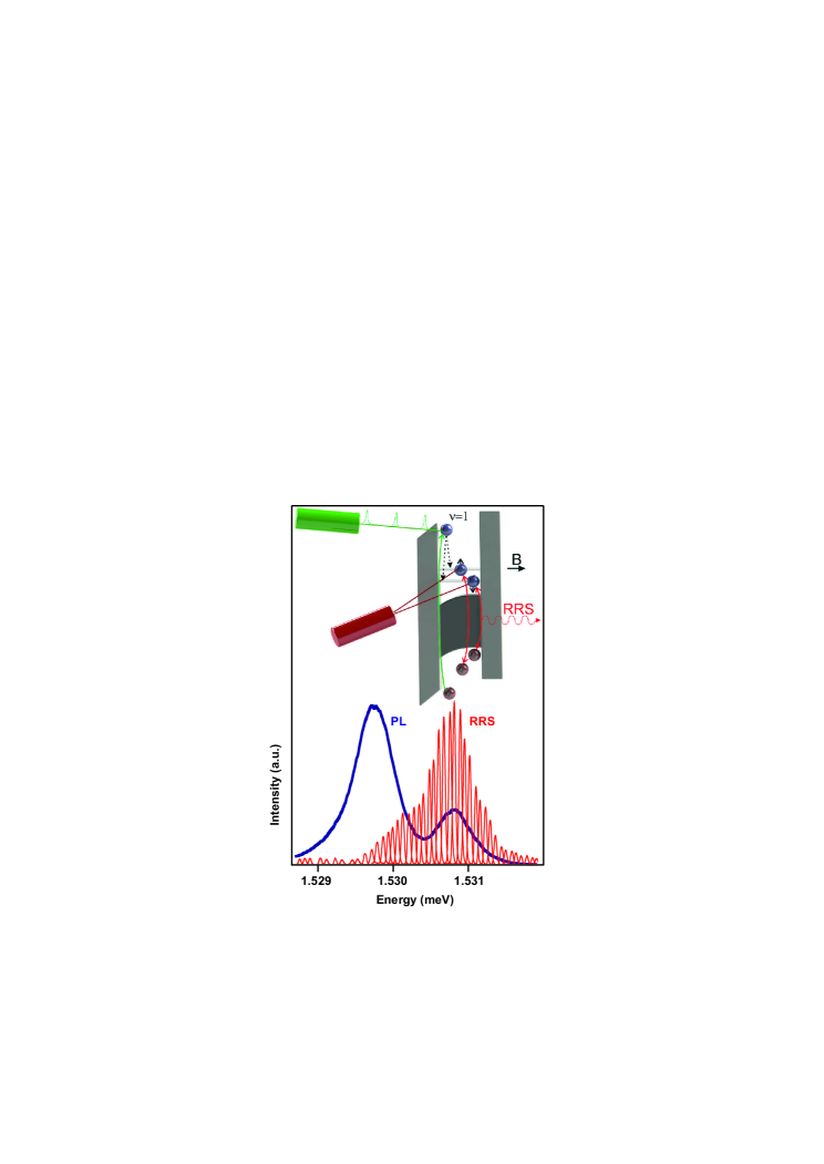
Figure 1: (top) A schematic diagram of the experimental setup. (bottom) Photoluminescence (PL) and resonant Rayleigh scattering spectra obtained 5 ms after the heating laser pulse at a magnetic field of 11 T and a bath temperature of 1.6 K.

Several GaAs/AlGaAs quantum wells of $18-20\,$nm width 2DES with an electron density in the range of $1.5-4\!\times\!10^{11}$cm$\!{}^{-2}$ were studied (dark mobility varying from $1$ to $3\!\times\!10^{6}\,$cm²/Vs). The experimental technique used to produce a nonequilibrium spin system utilized short ($<\!\!1\,$ns) powerful laser pulses with the photon energy far above the forbidden gap in GaAs (peak power was $10^{4}$J/cm²), see the illustration in Fig 1. By relaxing to the ground state, the high-energy electrons heat the 2DES. The experiment has two options: (i) the characteristic time required to cool down the 2DES is longer than the spin relaxation time (then the relaxation rate can not be accurately measured) and (ii) the spin relaxation time is longer than the time required to cool down the 2DES. In the latter case, the spin relaxation rate is measured directly. This condition can be satisfied at magnetic fields $B\!\geq\!9\,$T. The optically heated 2DES relaxes to a nonequilibrium spin depolarized state. A continuous wave radiation resonating with the optical transitions involving electron and heavy-hole states in the zero Landau levels monitors the 2DES spin by resonant Rayleigh scattering (RRS), as described in Ref. Kulik12 (Fig. 1). The ratio of the Rayleigh scattering cross sections for the two allowed optical transitions (+1/2, -3/2) and (-1/2, +3/2) allows the heating laser power to be tuned in such a way that the nonequilibrium 2DES proves to be in an unpolarized state after cooling down.

The dynamics of the RRS signal in the $\nu\!=\!1$ quantum Hall ferromagnet reveals nonmonotonic behavior. Within the first few nanoseconds after the laser pulse, the RRS signal superimposes on the nonresonant photoluminescence induced by the pulse. The 2DES is then heated during the first $10\,$ns. This process is accompanied by a complete loss of the RRS intensity (Fig. 2). During the following $40\,$ns the RRS signal returns to the initial value, thus indicating that the temperature of the 2DES reaches the bath temperature. The RRS signal then again diminishes due to the 2DES spin relaxation to the equilibrium state. Finally, the RRS signal is saturated at a stable level, the magnitude of which depends on the bath temperature. The stable level characterizes the equilibrium spin state of the 2DES (Fig. 2). Measuring its magnitude at different temperatures allows us to determine the temperature dependence of the 2DES equilibrium spin polarization. It reproduces the well-known experimental results obtained with the nuclear magnetic resonance technique (Fig. 2).

Subtracting the equilibrium RRS signal from the total RRS signal, one obtains the spin relaxation rate as a function of the nonequilibrium spin density (Fig. 2). We observed a number of significant effects that reduced the number of possible mechanisms accounting for the spin relaxation in 2DES. First, the relaxation time was not dependent on the electron temperature, whereas the amount of relaxed electrons changed significantly. [For example, at $4.2\,$K the relaxation is nearly exhausted (Fig. 2).] Second, within the experimental accuracy, we found no appreciable changes in the relaxation time versus the nonequilibrium spin density (Fig. 2).

Another finding is the long spin relaxation time, which was more than one order of magnitude longer than any known experimental results Alphenaar98 ; Fukuoka ; Nefyodov . We believe that such a striking discrepancy between our and other experimental data was due to the different physical quantities measured. Our technique directly aims at the spin relaxation from the upper to the lower spin sublevel in a nonequilibrium strongly interacting 2DES , whereas other experimental techniques, such as the paramagnetic resonance and the Kerr rotation, focus on the spin dephasing of a single or few noninteracting spin excitons.

Figure 2: a) Envelopes for nonequilibrium (open dots) and equilibrium (solid dots) RRS spectra measured at B=11 T and T=1.6 K in 50 ns and 5 $\mu$s after the heating laser pulse, respectively. The arrow indicates the maximum of the PL line for the electron-hole transition associated with the lowest spin Landau sublevel where the RRS signal dynamics are measured. b) The RRS dynamics for the stable temperature points of 0.4, 1.6, 2.2, and 4.2 K (the RRS signals at different temperatures are normalized to give equal intensities 50 ns after the heating laser pulse). c) The RRS signal intensity minus the magnitude of the saturated RRS signal in logarithmic scale vs time after the heating laser pulse at different bath temperatures (point colors are the same as in b)). d) The equilibrium spin polarization (large spheres) obtained using the magnitudes of saturated RRS signals at different bath temperatures (the equilibrium polarization at 0.4 K is taken as 1). For comparison, the equilibrium spin polarization measured with the nuclear magnetic resonance technique in Ref. [Barrett, ] at a similar Zeeman energy (small spheres connected by the thin line) is shown. The thick solid line indicates single particle (without Coulomb correlations) equilibrium spin polarization.

Spin excitons are true eigen states of the quantum Hall ferromagnet. A comparative analysis of various temperature-independent relaxation channels was recently reported di12 . We conclude that for $B\!<\!15\,$T, the relaxation channel is determined by both the SO coupling providing the spin nonconservation and the interaction with the smooth random potential violating the momentum conservation. Indeed, a similar relaxation mechanism was already theoretically discussed di04 ; di12 , but with one significant difference – smooth random potential was considered to be weak and, therefore, producing no effect on the energy spectrum of spin excitons or on their energy distribution. This was considered to be the cause of the two-exciton scattering dissipation mechanism. As a result, this theoretical model leads to a nonexponential relaxation law, $\sim 1/(1\!+\!t/\tau)$ di04 ; di12 , which thereby contradicts the observed exponential relaxation. Some results, however, can be still utilized. Namely, let us consider a 2D domain with area $L^{2}$ where $L$ is much larger than the characteristic correlation length $\Lambda$ of the correlator $K({\bf r})\!=\!\langle\varphi({\bf r})\varphi(0)\rangle$ [$\varphi({\bf r})$ describes the external smooth random potential; $\langle\varphi({\bf r})\rangle\,\equiv\,0$ is assumed]. In this case, the matrix element for the transition from the two exciton state with wave vectors ${\bf q}_{1}$ and ${\bf q}_{2}$ to a single exciton state with ${\bf q}^{\prime}$ is $\left|{\cal M}({\bf q}_{1},{\bf q}_{2},{\bf q}^{\prime})\right|^{2}\!\!=\!{}4\pi\overline{K}({q}^{*}\!){{q^{*}}^{2}(u^{2}\!+\!v^{2})}/{N_{\phi}^{2}}$, where ${\bf q}^{*}\!=\!{\bf q}_{1}\!+\!{\bf q}_{2}\!-\!{\bf q}^{\prime}$; $u\!=\!\sqrt{2}\alpha/l_{B}\hbar\omega_{c}$ and $v\!=\!\sqrt{2}\beta/l_{B}\hbar\omega_{c}$ are the dimensionless SO constants [$l_{B}$ – magnetic length, $\omega_{c}$ – cyclotron frequency, wave vectors are measured in $1/l_{B}$ units]. We have taken the corresponding SO term in the single electron Hamiltonian as ${\hat{H}}_{\rm SO}=\alpha\left(\hat{{\bf q}}\times\hat{\mbox{\boldmath$\sigma$}}\right)_{\!z}\!+\!\beta\left(\vphantom{\left(\hat{{\bf q}}\times\hat{\mbox{\boldmath$\sigma$}}\right)}\hat{q}_{y}\hat{\sigma}_{y}\!-\!{\hat{q}}_{x}\hat{\sigma}_{x}\right),\>\mbox{where}\>\;\hat{{\bf q}}\!=\!-i{\mbox{\boldmath$\nabla$}}\!+\!e{\bf A}/c\hbar$, $N_{\phi}\!=\!L^{2}/2\pi l_{B}^{2}$ is the number of electron states in one spin sublevel, and $\overline{K}({q})\!=\!\frac{1}{(2\pi)^{2}}\!\int\!K({\bf r})e^{-i{\bf q}{\bf r}}d^{2}{r}$ is the correlator Fourier component. The annihilation is defined by an elementary process in which two spin excitons with ${\bf q}_{1}$ and ${\bf q}_{2}$ merge, and a new spin exciton arises with the energy ${\cal E}^{\prime}$ equal to the sum of energies ${\cal E}_{1}\!+\!{\cal E}_{2}$ for merging spin excitons. The annihilation probability, if both excitons are within the domain $L\!\times\!L$, is calculated with the standard formula $1/\tau({\bf q}_{1},{\bf q}_{2})\!=\!\!\sum_{{\bf q}^{\prime}}\!\frac{2\pi}{\hbar}\left|{\cal M}({\bf q}_{1},{\bf q}_{2},{\bf q}^{\prime})\right|^{2}\!\delta\!\left({\cal E}_{1}\!+\!{\cal E}_{2}\!-\!{\cal E}^{\prime}\right)$.

If the temperature is rather low, then to calculate the total relaxation rate one has to know the quasi-equilibrium distribution of “cold” spin-excitons determined not only by temperature but also by the random potential (i.e., in the state where they are cooled but not annihilated, because the cooling processes that do not involve the spin flip are considered to occur much faster). The problem of finding this distribution in real space cannot be precisely solved, and we are only able to present a comprehensive estimate. Now the exciton momentum is no longer a good quantum number, and from the distribution in the conjugate space one should return to the spin-exciton distribution in real space characterized by the density $n({\bf r})$. From this point of view, the values ${\bf q}_{1}$, ${\bf q}_{2}$ and ${\bf q}^{\prime}$ entering the expressions above must be reexamined.

The following study is very similar to that presented recently di13 . First we show how the random smooth potential influences the spin-exciton energy. Let the random potential be smooth (i.e., $l_{B}\!\ll\!\Lambda$). We consider a small domain $l\times l$ ($l_{B}\!\ll\!l\!\ll\!\Lambda$ ) and use a linear-gradient approximation: ${\hat{\varphi}}\!=\!-(l_{B}/\hbar){\mbox{\boldmath$\nabla$}}\!\varphi\!\times\!{\hat{\bf\cal P}}$ within this domain, where ${\hat{\bf\cal P}}$ is a ‘generalized’ momentum operator of the magneto-exciton di13 . Within the approximation of the first-order gradient expansion, the smooth potential does not change exciton states and conserves the quantum number ${\bf q}$. In addition, the linear potential does not contribute to the value $\overline{K}({q}){q^{2}}$ [proportional to the Fourier component of the correlator $\langle{\mbox{\boldmath$\nabla$}}^{2}\!\!\varphi({\bf r})\varphi(0)\rangle$]. It does, however, determine the electro-dipole part of the exciton energy so that the latter is $\epsilon_{\rm Z}\!+\!q^{2}/2M_{\rm x}\!-\!{\bf d}{\mbox{\boldmath$\nabla$}}\!\varphi$, where ${\bf d}\!=\!l_{B}({\bf q}\!\times\!{\hat{z}})$ is the dipole moment, ($\epsilon_{\rm Z}\!=\!g\mu_{B}B$ is the Zeeman gap, and $1/M_{\rm x}$ is the exciton inverse mass; $q$ is in the $1/l_{B}$ units). After cooling down, but before annihilation, the exciton in the vicinity of point ${\bf r}$ acquires wave vector ${\bf q}_{m}\!\equiv\!M_{\rm x}l_{B}{\hat{z}}\!\times\!{\mbox{\boldmath$\nabla$}}\!\varphi({\bf r})$ and “gets stuck” in the smooth random potential with the exciton energy ${\cal E}_{m}\!=\!\epsilon_{\rm Z}-q_{m}^{2}/2M_{\rm x}$. The inverse ‘local’ relaxation time $1/\tau({\bf q}_{1},{\bf q}_{2})$ is calculated with substitution ${\bf q}_{1}\!=\!{\bf q}_{2}\!=\!{\bf q}_{m}({\bf r})$, and as a result, if the correlator is Gaussian, $K(r)\!=\!\Delta^{2}e^{-r^{2}/\Lambda^{2}}\!$, one obtains $\tau({\bf r})\!=\!N_{\phi}{\cal T}({\bf r})$, where here and in the expressions above one has to change from $N_{\phi}\!=\!L^{2}/2\pi l_{B}^{2}$ to $N_{\phi}\!=\!l^{2}/2\pi l_{B}^{2}$. Thus, one finds

$$\frac{1}{{\cal T}({\bf r})}=\frac{M_{\rm x}\Delta^{2}\Lambda^{2}(u^{2}\!+\!v^{2})}{\hbar l_{B}^{2}}\quad\qquad{}\qquad\qquad$$

$$\times\int_{q^{\prime}_{\rm min}}^{q^{\prime}_{\rm max}}\!\!\frac{\exp{\![-q^{2}(q^{\prime})\Lambda^{2}/4]}\,q^{2}(q^{\prime})\,q^{\prime}dq^{\prime}}{\sqrt{q_{m}^{2}q^{\prime 2}-(q^{\prime 2}/2+q_{m}^{2}-\epsilon_{\rm Z}M_{\rm x})^{2}}}\,.\vspace{-1mm}$$ (1)

Here $q_{m}^{2}({\bf r})\!=\!(\!M_{\rm x}l_{B}\!{\mbox{\boldmath$\nabla$}}\!\varphi)^{2}$, $q^{\prime}_{\rm min}\!=\!|\sqrt{2M_{\bf x}{\cal E}_{m}}\!-\!q_{m}|$, $q^{\prime}_{\rm max}\!=\!\sqrt{2M_{\bf x}{\cal E}_{m}}\!+\!q_{m}$, and $q^{2}(q^{\prime})\!=\!4\epsilon_{\rm Z}M_{\rm x}\!-\!q^{\prime 2}$ foot .

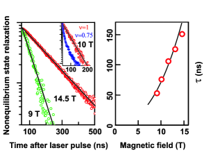
Figure 3: (left) The RRS signal intensity minus the magnitude of the saturated RRS signal in the logarithmic scale (points) vs time after the heating laser pulse measured for B=9 and 14.5 T. Solid lines being exponential fits to the experimental data. Purple rings on the inset represent the RRS signal corresponding to spin-relaxation dynamic at $\nu\!=\!0.75$ and $B\!=\!10\,$T. The relaxation is actively non-exponential in the case. For comparison, we also show the $\nu\!=\!1$ data at the same magnetic field. (right) The relaxation time constant for the quantum Hall ferromagnet vs magnetic field (open dots). Solid line is the theoretical fit (value of ${\EuScript T}$) to the experimental data obtained with the parameter set indicated in the text.

The experimentally measurable quantity – the total relaxation rate – is calculated by multiplying the probability $1/\tau({\bf r})$ by the probability of finding two spin excitons within the $l\!\times\!l$ domain, $\times n^{2}({\bf r})l^{4}$, and then by summation over all domains. The latter means substitution $l^{2}\!\to\!d{\bf r}$ and integration over ${\bf r}$:

$$-dN_{\rm x}/dt\!=\!2\pi l_{B}^{2}\!\int\!n^{2}({\bf r})/{\cal T}({\bf r})d{\bf r}.\vspace{-2mm}$$ (2)

Thus, we have a complex problem of finding the density distribution $n({\bf r})$ and calculating the integral in Eq. (2). A quasi-equilibrium distribution $n({\bf r})$ is determined by fast transition processes preceding the spin exciton annihilation: cooling due to the electron-phonon coupling and simultaneous drifting in the presence of a smooth random field. This field influencing the exciton energy ${\cal E}_{m}$ is actually not $\varphi$ but $({\mbox{\boldmath$\nabla$}}\!\varphi)^{2}\!$, representing a non-Gaussian case.

We obtain the required estimate in two steps. First, let us change from ${\cal T}({\bf r})$ to the averaged value ${\tilde{\cal T}}$ by substituting for $q_{m}^{2}$ in Eq. (1) the mean quantity $\langle q_{m}^{2}\rangle$ calculated with the averaging procedure $\langle q_{m}^{2}\rangle/(M_{\rm x}l_{B})^{2}\!=\!\langle({\mbox{\boldmath$\nabla$}}\!\varphi)^{2}\rangle\!\equiv\!\!2(\Delta/\Lambda)^{2}$, which is valid for the Gaussian potential $\varphi$. Second, for a spatially fluctuating density $n({\bf r})\!\equiv\!N_{\rm x}/\!L^{2}\!+\!\delta n({\bf r})$, we estimate the integral $\int\!\!n^{2}({\bf r})d{\bf r}\!\equiv\!N_{\rm x}^{2}/\!L^{2}\!+\!\int[\delta n({\bf r})]^{2}d{\bf r}$, where the last term is proportional to the spatial correlator $\langle\delta n({\bf r})\delta n(0)\rangle$ at ${\bf r}\!=\!0$. Should spin excitons form an ideal gas, this correlator would correspond to so-called white noise and would be equal to $\delta({\bf r})N_{\rm x}/L^{2}$ ll91 . In our case, the correlations are mostly determined by spatial fluctuations of the field $({\mbox{\boldmath$\nabla$}}\!\varphi)^{2}$: if it is energetically favorable to find a spin exciton at a point ${\bf r}_{0}$, then the density should be over the mean value, $\delta n({\bf r}_{0})\!>\!0$ in the neighborhood $|{\bf r}\!-\!{\bf r}_{0}|\!\lesssim\!\Lambda^{\prime}$. For an estimate, the $\delta({\bf r})$ function is replaced with a ‘hat’-function $e^{-r^{2}/{\Lambda^{\prime}}^{2}}\!\!/\pi{\Lambda^{\prime}}^{2}$. Intuitively, the estimate for $\Lambda^{\prime}$ is $\Lambda^{\prime}\!\simeq\!\Lambda/2$. As a result, we come to $\int[\delta n({\bf r})]^{2}\!d{\bf r}\!\sim\!4N_{\rm x}/\pi{\Lambda}^{2}$.

Thus, there are two contributions to the relaxation rate (2). The first contribution is a quadratic in $n_{\rm x}\!=\!2\pi l_{B}^{2}N_{\rm x}/L^{2}$ and is determined by the mean excitonic density, whereas the second contribution originates from the part of the fluctuations that is linear in $n_{\rm x}$:

$$-dn_{\rm x}/dt\sim n^{2}_{\rm x}/{\tilde{\cal T}}+8l_{B}^{2}n_{\rm x}/{\tilde{\cal T}}\Lambda^{2}.\vspace{-1mm}$$ (3)

Our theoretical approach is based on neglecting the inter-excitonic correlations. That is, $n_{\rm x}$ is assumed to be small, and the second term in Eq. (3) is thus dominant. Experimentally, the observed relaxation is well-exponential in time, even starting from the initial value $n_{\rm x}(0)\simeq 0.5$. So, semi-empirically, we conclude that the characteristic relaxation time is given by ${\EuScript T}\!=\!{\tilde{\cal T}}\Lambda^{2}/8l_{B}^{2}$. The material parameters can be evaluated using available data for similar quantum wells Larionov and by slightly varying the poorly known quantities: $\Delta$ and $\Lambda$, around their experimentally estimated values. The magnitude of $1/M_{\rm x}$ was borrowed from a recent experiment Kulik . In so doing, and to compare the theory with our experimental measurements, one could, for example, consider the following specific parameters quite reasonable for our experimental conditions: $\alpha\!=\!0.25\,$nm$\cdot$meV, $\beta\!=\!0.12\,$nm$\cdot$meV, $\epsilon_{\rm Z}\!=\!0.02B\,$meV, $1/M_{\rm x}\!=\!0.87B^{1/2}$meV ($B$ in Teslas), $\Delta\!=\!1.25\,$meV, and $\Lambda\!=\!32\,$nm. As a result, one obtains a specific dependence ${\EuScript T}(B)$ that nicely describes the experimental data (Fig. 3). Finally, note that the real temperature at which the employed ‘zero-temperature’ approach should be valid is estimated to be $T\!<\!{\langle q_{m}^{2}\rangle}/M_{\rm x}\!\sim\!M_{\rm x}(l_{B}\Delta/\Lambda)^{2}\!\simeq\!1\,$K.

Finally as a basis for a discussion we briefly concern the situation of a softer quantum Hall ferromagnet. In case the filling deviates from one, the spin polarization diminishes (see, e.g., an analysis in Ref.pl09 ), and drastic rearrangement of the ground state – emergence of a skyrmionic texture has to result in radical changes of excitations’ picture. In particular, it is known that additional spin-flip modes are observedga08 , and even only due this fact spin-relaxation physics becomes quite different compared to the $\nu\!=\!\!1$ case. Our intuitive opinion of this interesting but hardly studied relaxation problem enables us to think that the phase volume relevant to spin relaxation processes should grow if $\nu$ deviates from one – the relaxation thus occurs faster. Our experimental technique allows, e.g., to observe spin-relaxation dynamics at $\nu\!=\!0.75\,\,$(see the inset on Fig.  3).

In conclusion, we emphasize the importance of the presented results. Up to now, experimental physics have been focused on indirectly investigating the spin dephasing time of noninteracting spin excitons. In our study, we successfully prepared a nonequilibrium spin system that allows us to perform real-time monitoring of the spin dynamics. On the basis of these data and theoretical analysis, we describe a scenario for the relaxation and conclude that, in fact, there is no discrepancy between the experimental results and theoretical notions based on the concept of spin-exciton annihilation – the observed relaxation can be explained within the framework of the SO–smooth-disorder relaxation mechanism, and actually looks like effective inter–spin-exciton scattering. In addition, the long relaxation times, $100-150\,$ns, provide a chance to study a possible condensate state of nonequilibrium spin excitons.

The authors acknowledge the Russian Fund of Basic Research for support. S.D. is grateful to Serge Florens for valuable discussions concerning the fundamental problems of averaging under the conditions of a non-Gaussian smooth random potential.

References

- (1) I. Žutić, J. Fabian, S. Das Sarma, Review Mod. Phys. 76, 323 (2004).
- (2) M.I. D’yakonov and V.Yu. Kachorovskii, Sov. Phys. Semicond. 20, 110 (1986).
- (3) W.J.H. Leyland, G.H. John, R.T. Harley, M.M. Glazov, E.L. Ivchenko, D.A. Ritchie, I. Farrer, A.J. Shields, and M. Henini, Phys. Rev. B 75, 165309 (2007).
- (4) B.W. Alphenaar, H.O. Müller, and K. Tsukagoshi, Phys. Rev. Lett. 81, 5628 (1998).
- (5) D. Fukuoka, K. Oto, K. Muro, Y. Hirayama, and N. Kumada Phys. Rev. Lett. 105, 126802 (2010).
- (6) Yu.A. Nefyodov, A.A. Fortunatov, A.V. Shchepetilnikov, I.V. Kukushkin, JETP Letters 91, 357 (2010).
- (7) D.M. Frenkel, Phys. Rev. B 43, 14228 (1991); A.A. Burkov and L. Balents, Phys. Rev. B 69, 245312 (2004).
- (8) S. Dickmann, Phys. Rev. Lett. 93, 206804 (2004); S. Dickmann and S.V. Iordanskii, JETP 83, 128 (1996); JETP Lett. 70, 543 (1999).
- (9) S. Dickmann and T. Ziman. Phys. Rev. B 85, 045318 (2012).
- (10) L.V. Kulik, K. Ovchinnikov, A.S. Zhuravlev, V.E. Bisti, I.V. Kukushkin, S. Schmult, and W. Dietsche, Phys. Rev. B 85, 113403 (2012).
- (11) See http://link.aps.org/supplemental/10.1103/ PhysRevLett.110.166801 and references therein.
- (12) Eq. (1) in the limit just gives the value in Ref. di12 .
- (13) A.V. Larionov, A.S. Zhuravlev JETP Letters 97, 137 (2013).
- (14) L.V. Kulik, A.S. Zhuravlev, V.E. Kirpichev, V.E. Bisti, and I.V. Kukushkin, Phys. Rev. B 87, 045316 (2013).
- (15) S.E. Barrett, G. Dabbagh, L.N. Pfeiffer, K.W. West, and R. Tycko, Phys. Rev. Lett. 74, 5112 (1995).
- (16) L.D. Landau, E.M. Lifshitz, Statistical Physics, Course of Theoretical Physics, vol. 5, Pergamon Press, Oxford (1980).
- (17) P. Plochocka, J.M. Schneider, D.K. Maude, M. Potemski, M. Rappaport, V. Umansky, I. Bar-Joseph, J.G. Groshaus, Y. Gallais, and A. Pinczuk, Phys. Rev. Lett. 102, 126806 (2009).
- (18) Y. Gallais, J. Yan, A. Pinczuk, L.N. Pfeifer, and K.W. West, Phys. Rev. Lett. 100, 086806 (2008); I. K. Drozdov, L.V. Kulik, A.S. Zhuravlev, V.E. Kirpichev, I.V. Kukushkin, S. Schmult, and W. Dietsche, Phys. Rev. Lett. 104, 136804 (2010).