Analytical Equilibrium Solutions of Biochemical Systems with Synthesis and Degradation

Abstract

Analyzing qualitative behaviors of biochemical reactions using its associated network structure has proven useful in diverse branches of biology. As an extension of our previous work, we introduce a graph-based framework to calculate steady state solutions of biochemical reaction networks with synthesis and degradation. Our approach is based on a labeled directed graph $G$ and the associated system of linear non-homogeneous differential equations with first order degradation and zeroth order synthesis. We also present a theorem which provides necessary and sufficient conditions for the dynamics to engender a unique stable steady state.

Although the dynamics are linear, one can apply this framework to nonlinear systems by encoding nonlinearity into the edge labels. We answer open question from our previous work concerning the non-positiveness of the elements in the inverse of a perturbed Laplacian matrix. Moreover, we provide a graph theoretical framework for the computation of the inverse of a such matrix. This also completes our previous framework and makes it purely graph theoretical. Lately, we demonstrate the utility of this framework by applying it to a mathematical model of insulin secretion through ion channels and glucose metabolism in pancreatic $\beta$-cells.

1 Introduction

In recent years, many researchers have devoted their efforts to developing a systems-level understanding of biochemical reaction networks. In particular, the study of these chemical reaction networks (CRNs) using their associated graph structure has attracted considerable attention. The work led by Craciun and Feinberg on multistationarity [11, 13, 14, 12] and the work led by Mincheva and Roussel on stable oscillations [22, 23, 24] are two particularly influential approaches. For a good overview of the various graph theoretic developments, we direct the interested reader to the review provided in Domijan and Kirkilionis [15].

In this work, we focus on applications of graph theory, mainly the Matrix-Tree Theorem (MTT), for deriving equilibrium solutions (ES) for CRNs that fit within a Laplacian dynamics framework. The MTT-based framework was first applied in a biological context by King and Altman [18] to derive steady state rate equations in enzyme kinetics. This framework was then simplified and summarized into rules (known as Chou’s graphical rules [20]) by Chou and coworkers [8, 9, 10]. Chou [8] has also extended the framework for non-steady state enzyme-catalyzed systems.

The main disadvantage of Chou’s graphical rules is that they are only applicable if the underlying digraph structure is strongly connected, i.e., every vertex is reachable from every other vertex. This issue was solved and extended for general directed graphs (digraphs) by Mirzaev and Gunawardena in 2013 [25] and is applicable to the specific class of linear ordinary differential equations (ODEs) known as Laplacian dynamics. Systems described by Laplacian dynamics are created using a weakly connected digraph, $G$, with $n$ vertices, with labelled, directed edges, and without self loops. Note that by weakly connected we mean that the graph cannot be expressed as the union of two disjoint digraphs. If there is an edge from vertex $j$ to vertex $i$, we label it with $e_{ij}>0$, and with $e_{ij}=0$ if there is no such edge.

The Laplacian matrix (hereafter, a Laplacian $\mathcal{L}$) of given digraph $G$ is then defined as

$$\left(\mathcal{L}(G)\right)_{ij}=\begin{cases}e_{ij}&\text{if }i\neq j\\ -\sum_{m\neq j}e_{mj}&\text{if }i=j\,.\end{cases}$$ (1)

The corresponding Laplacian dynamics are then defined as

$$\frac{d\mathbf{x}}{dt}=\mathcal{L}(G)\cdot\mathbf{x}$$

where $\mathbf{x}=\left(x_{1},\cdots,x_{n}\right)^{T}$ is column vector of species concentrations at each vertex, $1,\cdots,n$. In a biochemical context one may think of vertices as different species and edges as rate of transformation from one species to another. However, we note that this framework is symbolic in nature in the sense that the mathematical description of the computed steady states is done without the specification of rate constants, i.e., edge weights $e_{ij}$. In other words, the only information about an individual $e_{ij}$ relevant to our approach is whether or not it is zero.

Laplacian matrices were first introduced by Kirchhoff in 1847 in his article about electrical networks [19]. Ever since then Laplacians have been studied and applied in various fields. For an example of studying the applications of Laplacians to spectral theory, we refer the interested reader to Bronski and Deville [5] in which they study the class of Signed graph Laplacians (a symmetric matrix, which is special case of above defined Laplacian).

In this article we will extend the framework intitially developed in [25] to investigate behaviors of Laplacian dynamics when zero-th order synthesis and first order degradation are added to the system. Specifically, we will examine the following dynamics,

$$\frac{d\mathbf{x}}{dt}=\mathcal{L}(G)\cdot\mathbf{x}-D\cdot\mathbf{x}+\mathbf{s}$$ (2)

where the degradation matrix $D$ is a diagonal matrix with $\left(D\right)_{ii}=d_{i}\geq 0$ and the synthesis vector $\mathbf{s}$ is a column vector with $\left(\mathbf{s}\right)_{i}=s_{i}\geq 0$. Hereafter, we refer to this new dynamics as synthesis and degradation dynamics (or simply as SD dynamics). In the biological networks literature this type of dynamics are often referred as inconsistent networks[21].

For these dynamics, several questions naturally arise. Under what conditions does this system have non-negative, stable ES solution? Moreover, how can we relate the ES solution to the underlying digraph structure of $G$ as we did for Laplacian dynamics without synthesis and degradation? Our goal is to answer these questions on a theoretical level as well as apply the result to real world CRN examples.

The outline of this work is as follows. We will first briefly review the main results of [16, 25] and present some additional notation (to be used in subsequent sections). In Section 3 we describe our main theoretical results and in Section 4 fully discuss the proof of an important result in Section 3.

In Section 5, we illustrate an application of these results to exocytosis cascade of insulin granules and glucose metabolism in pancreatic $\beta$-cells. Lastly, in Section 6, we conclude with a discussion of the implications of these results as well as plans for future work.

2 Preliminaries

In this section we briefly summarize the important results of Mirzaev and Gunawardena [25] and refer the interested reader to that article for proofs and more extensive discussion and interpretation. For the sake of clarity, we will preserve the original notation while we include some additional definitions that can be found in many introductory graph theory books.

Given a digraph $G$, we denote the set of vertices of $G$ with $\mathcal{V}(G)$ and we write $i\Longrightarrow j$ to denote the existence of a path from vertex $i$ to vertex $j$. If $i\Longrightarrow j$ and $j\Longrightarrow i$, vertex $i$ is said to be strongly connected to vertex $j$, and is denoted $i\Longleftrightarrow j$. A digraph $G$ is strongly connected if for each ordered pair $i,j$ of vertices in $G$, we have that $i\Longleftrightarrow j$. The strongly connected components (SCCs) of a digraph are the largest strongly connected subgraphs. Let $C[i]$ denote the SCC containing $i$, $i\in\mathcal{V}(C[i])$. Suppose we are given two SCCs, $C[i]$ and $C[j]$, if $i\Longrightarrow j$ we write $C[i]\preceq C[j]$ to denote that $C[i]$ precedes $C[j]$. This precedes relation is both reflexive and transitive. Moreover, the relation is also antisymmetric as $C[i]\preceq C[j]$ and $C[j]\preceq C[i]$ imply that $i\Longleftrightarrow j$ and $C[i]=C[j]$. From this, we can conclude that the precedes relation allows for a partial ordering of the SCCs. Accordingly, this allows us to identify so-called terminal SCCs (tSCC), which are those SCCs $C[i]$ such that, if $C[i]\preceq C[j]$ then $C[i]=C[j]$. These tSCCs are used in many other contexts, for example, they are also known as “attractors” of state transition graphs [4].

With this terminology, we can devise an insightful relabeling of the vertices of digraph $G$. Such a relabeling will transform the Laplacian matrix into one with a block lower-diagonal structure, which will prove convenient in our theoretical development. Suppose there are $q$ tSCCs out of a total of $p+q$ SCCs. Our goal is to relabel the vertices such that the first $p$ blocks of Laplacian matrix correspond to the $p$ non-terminal SCCs. Since the precedence relation, $\preceq$, is a partial ordering, there exists an ordering of the SCCs, $C_{1},\dots,C_{p+q}$, such that, if $C_{i}\preceq C_{j}$, then $i\leq j$. Since a tSCC cannot precede any other SCC, then the tSCCs can be in some arbitrary order $\{C_{i}\}_{i=p+1}^{p+q}$ (which will not impact our results). We denote $a_{i}$ as the number of vertices in $C_{i}$, and $m_{i}=\sum_{k=1}^{i}a_{k}$ as the partial sum of the $a_{i}$’s, (with $m_{0}=0$). Note that the $a_{i}$’s should add up to the number of vertices in digraph $G$, i.e. $\sum_{i=1}^{p+q}a_{i}=n$. Then the vertices of $C_{i}$ are relabeled using only indices $m_{i-1}+1,\dots,m_{i-1}+a_{i}$ for $i=1,\dots,p+q$. Consequently, the new Laplacian matrix, $\mathcal{L}(G),$ is constructed using the relabeled vertices. Since $i<j$ implies $C_{j}\not\preceq C_{i}$, the Laplacian of $G$ can be written in block lower-triangular form

$$\mathcal{L}(G)=\left(\begin{array}[]{ccc|ccc}\boxed{\mathcal{L}_{1}}&\mathbf{0}&\mathbf{0}&\mathbf{0}&\cdots&\mathbf{0}\\ \vdots&\ddots&\vdots&\vdots&\vdots&\vdots\\ +&+&\boxed{\mathcal{L}_{p}}&\mathbf{0}&\cdots&\mathbf{0}\\ \hline\cr+&\cdots&+&\boxed{\mathcal{L}_{p+1}}&\mathbf{0}&\mathbf{0}\\ \vdots&\vdots&\vdots&\vdots&\ddots&\vdots\\ +&\cdots&+&\mathbf{0}&\mathbf{0}&\boxed{\mathcal{L}_{p+q}}\end{array}\right)=\left(\begin{array}[]{c|c}N&\mathbf{0}\\ \hline\cr B&T\end{array}\right)\,,$$

where $+$ stands for some matrix with non-negative real entries, the submatrix $N$ is block lower-triangular with non-negative off-diagonal elements, $B$ is a matrix with non-negative elements, $\mathbf{0}$ is matrix of all zeros, and $T$ is also a block diagonal matrix such that

$$N=\left(\begin{array}[]{ccc}\boxed{\mathcal{L}_{1}}&&\mathbf{0}\\ \vdots&\ddots\\ +&+&\boxed{\mathcal{L}_{p}}\end{array}\right),\,T=\left(\begin{array}[]{ccc}\boxed{\mathcal{L}_{p+1}}&&\mathbf{0}\\ &\ddots\\ \mathbf{0}&&\boxed{\mathcal{L}_{p+q}}\end{array}\right)\,.$$ (3)

By the definition of the Laplacian matrix (see (1)) all off-diagonal elements are non-negative real numbers. The blocks in boxes on the main diagonal, denoted by $\mathcal{L}_{1},\dots,\mathcal{L}_{p+q}$, are the submatrices defined by restricting $\mathcal{L}(G)$ to the vertices of the corresponding SCCs, $C_{1},\dots,C_{p+q}$. Note that for $i=p+1,\dots,p+q$ each $\mathcal{L}_{i}$ is Laplacian matrix in its own, $\mathcal{L}_{i}=\mathcal{L}(C_{i})$ . However for the non-terminal SCCs, $\left\{C_{i}\right\}_{i=1}^{p}$, there is always at least one outgoing edge to some other SCC. This implies that for $i=1,\dots,p$ each matrix $\mathcal{L}_{i}$ is defined as the Laplacian of a corresponding SCC minus some non-zero diagonal matrix corresponding to outgoing edges from this SCC, $\mathcal{L}_{i}=\mathcal{L}(C_{i})-\Delta_{i}$ for some $\Delta_{i}\not\equiv 0$. In this case we call $\mathcal{L}_{i}$ a perturbed Laplacian matrix, or simply a perturbed matrix and note the following property of $\mathcal{L}_{i}$ (proven in [25]).

Remark 1.

The Perturbed Laplacian matrix of strongly connected graph $G$ is non-singular.

A directed spanning subgraph of digraph $G$ is a connected subgraph of $G$ that includes every vertex of $G$, so that any spanning subgraph which is at the same time is a tree is called directed spanning tree (DST) of the digraph $G$. We say that a DST, $\mathscr{T}$, is rooted at $i\in G$ if vertex $i$ is the only vertex in $\mathscr{T}$ without any outgoing edges, and denote the set of DSTs of digraph $G$ rooted at vertex $i$ with $\Theta_{i}(G)$. Thus $\Theta_{i}(G)$ is a non-empty set of spanning trees for a strongly connected digraph $G$. However, for an arbitrary digraph there maybe no spanning tree rooted at specific vertex, in which case $\Theta_{i}(G)=\emptyset$. In this case the corresponding element, $\mathcal{L}(G)_{(j)}$, is zero, where $\mathcal{L}(G)_{(ji)}$ denotes the $ji$-th minor of Laplacian matrix $\mathcal{L}(G)$ and is the determinant of the $(n-1)\times(n-1)$ matrix that results from deleting row $j$ and column $i$ of $\mathcal{L}(G)$.

Next we review the main theorem from [25] on which the results of this paper are based. The theorem utilizes the digraph structure of digraph $G$ to calculate minors of a Laplacian. The proof of this theorem can be found in several papers, and we direct readers to [25] for a proof with same notations as in this article.

Theorem 2.

(Matrix-Tree Theorem) If $G$ is digraph with $n$ vertices then the minors of its Laplacian are given by

$$\mathcal{L}(G)_{(ij)}=(-1)^{n+i+j-1}\sum_{\mathscr{T}\in\Theta_{j}(G)}P_{\mathcal{\mathscr{T}}}\,,$$

where $P_{\mathcal{\mathscr{T}}}$ is the product of all edge weights in the spanning tree $\mathscr{T}$.

An illustration of above theorem is depicted in Figure 1, where $\mathcal{L}(G)_{(23)}$ and $\mathcal{L}(G)_{32}$ minor of $\mathcal{L}(G)$ are computed using spanning trees of digraph $G$. Consequently, the MTT implies that the $ij$-th minor of the Laplacian (up to sign) is the sum of all $P_{\mathcal{\mathscr{T}}}$ for each spanning tree, $\mathscr{T}$, rooted at vertex $j$. Since all edges of the digraph $G$ are non-negative numbers (zero only if there is no such edge), then the expression $\rho_{i}^{G}=\sum_{\mathscr{T}\in\Theta_{i}(G)}P_{\mathscr{T}}$ will always be non-negative. If $G$ is strongly connected then $\Theta_{i}(G)\neq\emptyset$, so $\rho_{i}^{G}$ is strictly positive.

(a) A digraph $G$ with its set of spanning trees rooted at each of its vertices. The root node is bolded in each spanning tree.

$\mathcal{L}(G)=\left(\begin{array}[]{ccc}-a&0&c\\ a&-b&\leavevmode\hbox to18.85pt{\vbox to18.85pt{\text{[drawing]}}}\\ 0&\leavevmode\hbox to18.22pt{\vbox to18.22pt{\text{[drawing]}}}&-c-d\end{array}\right)$

(b) Associated Laplacian matrix of $G$. Two minors of the Laplacian matrix, $\mathcal{L}(G)_{(23)}$ and $\mathcal{L}(G)_{(32)}$, are calculated using the Matrix-Tree Theorem.

Figure 1: Illustration of Matrix-Tree Theorem

Uno in his article [30] provided an algorithm for enumerating and listing all spanning trees of a general digraph and Ahsendorf et al. [2] utilized Uno’s algorithm to compute minors of Laplacian matrix using the Matrix-Tree theorem. Having an implementation of the MTT available, one can then calculate the kernel elements of the Laplacian, $\mathcal{L}(G)$, using the following two fairly well known Propositions (see [25] for proofs).

Proposition 3.

If $G$ is strongly connected graph, then $\ker\mathcal{L}(G)=span\left\{\bm{\rho}^{G}\right\}$, where $\bm{\rho}^{G}$ is column vector with $\left(\bm{\rho}^{G}\right)_{i}=\rho_{i}^{G}>0$.

Here, the kernel is defined in the conventional sense, $\ker\mathcal{L}(G)=\left\{x\in\mathbb{R}^{n\times 1}:\,\mathcal{L}(G)\cdot x=\mathbf{0}\right\}$. Moreover, Proposition 3 guarantees that a kernel element has all positive elements, a fact which is not immediately obvious using standard linear algebraic methods. When $G$ is not a strongly connected digraph, the kernel elements of $\mathcal{L}(G)$ are constructed using kernel elements of its tSCCs. Specifically, since for $i=1,\cdots,q$ each $\mathcal{L}_{p+i}=\mathcal{L}(C_{p+i})$ is a Laplacian matrix on its own, by Proposition 3 there exists $\bm{\rho}^{C_{p+i}}\in\mathbb{R}_{>0}^{a_{p+i}\times 1}$ such that $\mathcal{L}_{p+i}\cdot\bm{\rho}^{C_{p+i}}=\mathbf{0}$ and $a_{i}$ is the number of vertices in $C_{i}$. Then we can extend this vector to $\bar{\bm{\rho}}^{C_{p+i}}\in\mathbb{R}_{>0}^{n\times 1}$ by setting all entries with indices outside $C_{p+i}$ to zero:

$$\left(\bar{\bm{\rho}}^{C_{p+i}}\right)_{k}=\begin{cases}\left(\bm{\rho}^{C_{p+i}}\right)_{k-m_{p+i-1}}&\text{if }m_{p+i-1}\leq k\leq m_{p+i}\\ 0&\text{otherwise}\end{cases}$$ (4)

Since $\mathcal{L}(G)$ has lower-block diagonal structure and since $\mathcal{L}_{p+i}\cdot\bm{\rho}^{C_{p+i}}=\mathbf{0}$ for each $i=1,\cdots,q$ we have $\mathcal{L}(G)\cdot\bar{\bm{\rho}}^{C_{p+i}}=\mathbf{0}$. This can be summarized in the following Proposition:

Proposition 4.

For any graph $G$,

$$\ker\mathcal{L}(G)=span\left\{\bar{\bm{\rho}}^{C_{p+1}},\dots,\bar{\bm{\rho}}^{C_{p+q}}\right\}\,,$$

and $\dim\ker\mathcal{L}(G)=q$

To prove stability of the steady states we will use the following theorem and corollary, which provides sufficiency conditions for the solution to a dynamical system $d\mathbf{x}/dt=A\cdot\mathbf{x}$ coupled with initial condition $\mathbf{x}(0)=\mathbf{x}_{0}$ to converge to a steady state (proof in [25]). Typically, the stability of a dynamics depends on the sign of the real parts of the eigenvalues of $A$ as well as the algebraic and geometric multiplicities of the zero eigenvalue.

Theorem 5.

Suppose that the real matrix $A$ satisfies following two conditions

1. If $\lambda$ is an eigenvalue of $A$, then either $\lambda=0$ or $Re(\lambda)<0$

2. $alg_{A}(0)=geo_{A}(0)$, where $alg_{A}(0)$ and $geo_{A}(0)$ are the algebraic and geometric multiplicities of zero eigenvalue, respectively.

Then the solution of $d\mathbf{x}/dt=A\cdot\mathbf{x}$ converges to a steady state as $t\to\infty$ for any initial condition.

Corollary 6.

The Laplacian of a weakly connected digraph satisfies conditions of Theorem 5. Moreover, $geo_{\mathcal{L}(G)}\left(0\right)=alg_{\mathcal{L}(G)}\left(0\right)=q$, where $q$ is number of tSCCs of $G$.

With these preliminary results in hand we provide stability analysis for the SD dynamics as well as a graph theoretical algorithm for the computation of steady states.

3 Theoretical Development

In this section we will provide a thorough analysis of the synthesis and degradation dynamics (SD dynamics), (4), that we defined earlier. Suppose now that we add additional edges to core digraph, $G$,

$$\overset{s_{i}}{\longrightarrow}i\>,\,i\overset{d_{i}}{\longrightarrow}$$

corresponding to zeroth-order synthesis and first-order degradation, respectively. Each vertex can have any combination of synthesis and degradation edges and the dynamics can now be described by the following system of linear ordinary differential equations (ODEs):

$$\frac{d\mathbf{x}}{dt}=\mathcal{L}(G)\cdot\mathbf{x}-D\cdot\mathbf{x}+\mathbf{s}\,.$$ (5)

Here $\mathcal{L}(G)$ is the Laplacian matrix of the core digraph $G$, $D$ is a diagonal matrix with $\left(D\right)_{ii}=d_{i}$, and $\mathbf{s}$ is a column vector with $\left(\mathbf{s}\right)_{i}=s_{i}$, using the convention that $d_{i}$ or $s_{i}$ is zero if the corresponding partial edge at vertex $i$ is absent.

The presence of synthesis without degradation yields unstable dynamics. Therefore, whenever we have $D\equiv\mathbf{0}$ we assume that $\mathbf{s}\equiv\mathbf{0}$. In this case the system reduces to Laplacian dynamics, for which a thorough analysis was given in [25]. From now on we will assume that at least one element of $D$ is nonzero.

Proposition 7.

The dynamics defined by Equation (5) have a unique solution for a given initial condition.

Proof.

This can easily be verified as the right hand side of the dynamics, $f(\mathbf{x})=\mathcal{L}(G)\cdot\mathbf{x}-D\cdot\mathbf{x}+\mathbf{s}$ is affine in $\mathbf{x}$ and thus also Lipschitz continuous. Thus the existence of unique continuous solution is guaranteed. ∎

The next question to be answered is to identify the conditions under which the SD dynamics possess steady state solution(s). In order to derive the necessary and sufficient conditions for existence of steady state solution we define a complementary digraph, $G^{\star}$, which is formed by defining new vertex, $\star$, such that

$$\star\ce{->[s_{i}]}i\>\mbox{ or }\,i\ce{->[d_{i}]}\star$$

For the sake of simplicity we will divide our results into two cases: when $G^{\star}$ is a strongly connected digraph and when it is not strongly connected.

3.1 Strongly connected case

Assume that complementary digraph $G^{\star}$ is strongly connected. Let $F$ denote the matrix of the Laplacian minus the degradation matrix $D$:

$$F=\mathcal{L}(G)-D=\left(\begin{array}[]{ccc|ccc}\boxed{\mathcal{L}_{1}-D_{1}}&\cdots&\mathbf{0}&\mathbf{0}&\cdots&\mathbf{0}\\ \vdots&\ddots&\vdots&\vdots&\ddots&\vdots\\ +&\cdots&\boxed{\mathcal{L}_{p}-D_{p}}&\mathbf{0}&\cdots&\mathbf{0}\\ \hline\cr+&\cdots&+&\boxed{\mathcal{L}_{p+1}-D_{p+1}}&\mathbf{0}&\mathbf{0}\\ \vdots&\ddots&\vdots&\vdots&\ddots&\vdots\\ +&\cdots&+&\mathbf{0}&\mathbf{0}&\boxed{\mathcal{L}_{p+q}-D_{p+q}}\end{array}\right)$$ (6)

Suppose that there is some index $m\in\{p+1,\dots,p+q\}$ for which $D_{m}\equiv 0$. Then $\mathcal{L}_{m}-D_{m}=\mathcal{L}_{m}=\mathcal{L}(C_{m})$, which implies that $C_{m}$ is preserved as a tSCC in the complementary digraph $G^{\star}$. In this case, the vertices corresponding to the tSCC $C_{m}$ cannot be reached from any other SCC of $G^{\star}$, which in turn contradicts the fact that graph $G^{\star}$ is strongly connected. Thus each matrix $\mathcal{L}_{i}-D_{i}$ is a perturbed Laplacian matrix of some strongly connected digraph, so that from Remark 1 each $\mathcal{L}_{i}-D_{i}$ is a non-singular matrix for $i=p+1,\cdots,p+q$. For $i=1,\cdots,p$ as each of the $\mathcal{L}_{i}$’s is already a perturbed matrix, “perturb”-ing them further does not change the fact that they are non-singular. Thus the matrix $F$ is a non-singular matrix, since its diagonal components are all non-singular matrices and the unique steady state solution is given algebraically as

$$\mathbf{x}_{{\scriptscriptstyle ES}}=-(\mathcal{L}(G)-D)^{-1}\cdot\mathbf{s}\,.$$ (7)

However, we are interested in computing the ES by means of graph theory. Towards this end, we define a change of variables

$$\mathbf{x}=\mathbf{y}-(\mathcal{L}(G)-D)^{-1}\cdot\mathbf{s}\,.$$

This substitution transforms the original SD dynamics into

$$\frac{d\mathbf{y}}{dt}=(\mathcal{L}(G)-D)\cdot\mathbf{y}\,.$$ (8)

From Proposiotion 6 we know that eigenvalues of the Laplacian, $\mathcal{L}(G)$, satisfy $Re(\lambda)\leq 0$, where equality holds if and only if $\lambda=0$. The proof of this result follows from applying the Gershgorin theorem to the columns of the matrix $\mathcal{L}(G)$. Then the matrix $D$ in $\mathcal{L}(G)-D$ shifts the centers of the Gershgorin discs further to left on the real line without changing their radii, so we will still have $Re(\lambda)\leq 0$ for eigenvalues of the matrix $\mathcal{L}(G)-D$. On the other hand, the matrix $\mathcal{L}(G)-D$ is non-singular, so it follows that $Re(\lambda)<0$. This result in turn implies that solution of the system given in (8) converges to the trivial steady state, $\mathbf{y}_{{\scriptscriptstyle ES}}=0$. Thus we can now state the following theorem.

Theorem 8.

Given a strongly connected digraph $G$, the SD dynamics (5) have a unique stable steady state solution.

The symbolic computation of the ES solution using (7) can be very expensive even for small number of vertices. Therefore we restate an algorithm, given in [16], which uses graphical structure of graph $G^{\star}$ to calculate steady state solution given in (7).

Let $\mathbbm{1}=(1,\cdots,1)^{T}$ be a vector of all ones. At steady state we have $\frac{d\mathbf{x}}{dt}=\mathbf{0}$ and using the fact that $\mathbbm{1}^{T}\cdot\mathcal{L}(G)=\mathbf{0}$ it follows from (2) that

$$d_{1}x_{1}+\dots+d_{n}x_{n}=s_{1}+\dots+s_{n}\,.$$ (9)

In other words at steady state we should have an overall balance in synthesis and degradation. The Laplacian $\mathcal{L}(G^{\star})$ of the digraph $G^{\star}$ can then be related to the Laplacian $\mathcal{L}(G)$ of the digraph $G$

$$\mathcal{L}(G^{\star})=\left(\begin{array}[]{c|c}\mathcal{L}(G)&\mathbf{0}\\ \hline\cr\mathbf{0}&\mathbf{0}\end{array}\right)+\left(\begin{array}[]{c|c}-D&\mathbf{s}\\ \hline\cr\mathbbm{1}^{T}\cdot D&-\mathbbm{1}^{T}\cdot\mathbf{s}\end{array}\right)$$ (10)

Suppose now that we have overall balance in synthesis and degradation then using (10) it is easy to see that $(x_{1},\cdots,x_{n},1)$ is a steady state of

$$\frac{d\mathbf{x}}{dt}=\mathcal{L}(G^{\star})\cdot\mathbf{x}$$ (11)

if and only if $(x_{1},\cdots,x_{n})$ is a steady state of SD dynamics given in (5). Since $G^{\star}$ is strongly connected, the MTT provides a basis element for the kernel of the Laplacian matrix $\mathcal{L}(G^{\star})$, $\ker\left\{\mathcal{L}(G^{\star})\right\}=\text{span}\{\bm{\rho}^{G^{\star}}\}$ [16]. Consequently, the unique steady state $\mathbf{x}_{{\scriptscriptstyle ES}}$ is given by

$$\left(\mathbf{x}_{{\scriptscriptstyle ES}}\right)_{i}=\frac{\left(\bm{\rho}^{G^{\star}}\right)_{i}}{\left(\bm{\rho}^{G^{\star}}\right)_{\star}}$$ (12)

Since any steady state solution of (11) can be written as scalar multiple of kernel element, $\bm{\rho}^{G^{\star}}$, that single degree of freedom is used to guarantee that $\left(\mathbf{x}_{{\scriptscriptstyle ES}}\right)_{\star}=1$ (synthesis and degradation vertex, $\star$). This condition also ensures that overall balance in synthesis and degradation (9) is satisfied.

3.2 General Case

In contrast to the strongly-connected case, the steady state solutions do not always exist in the general case. First, we will derive conditions to assure the existence of a steady state solution. Then, we will show that provided we have a steady state solution $\mathbf{x}_{{\scriptscriptstyle ES}}$, the system converges to this $\mathbf{x}_{{\scriptscriptstyle ES}}$ as $t\to\infty$. Third, we provide a framework for construction of $\mathbf{x}_{{\scriptscriptstyle ES}}$ using the underlying graph structure of graph $G$ with illustration of results using a hypothetical example.

In the case that the digraph $G^{\star}$ is not strongly connected, in the partition of the matrix $F$ (6) there is at least one $i\in\left\{p+1,\dots,p+q\right\}$ such that $D_{i}\equiv\mathbf{0}$. Let $\left\{i_{1},\cdots,i_{k}\right\}\subseteq\left\{p+1,\cdots,p+q\right\}$ be a set for which $D_{i_{1}}=\dots=D_{i_{k}}\equiv\mathbf{0}$, then we can relabel the vertices corresponding to the tSCC such that matrices $\mathcal{L}_{i_{1}},\dots,\mathcal{L}_{i_{k}}$ are positioned in the lower right of matrix $F$,

$$F=\mathcal{L}(G)-D =\left(\begin{array}[]{ccc|ccc}\boxed{\mathcal{L}_{1}-D_{1}}&\cdots&\mathbf{0}&\mathbf{0}&\cdots&\mathbf{0}\\ \vdots&\ddots&\vdots\\ +&+&\boxed{\mathcal{L}_{p+q-k}-D_{p+q-k}}&\mathbf{0}&\cdots&\mathbf{0}\\ \hline\cr+&\cdots&+&\boxed{\mathcal{L}_{p+q-k+1}}&\cdots&\mathbf{0}\\ \vdots&\ddots&\vdots&\vdots&\ddots&\vdots\\ +&\cdots&+&\mathbf{0}&\cdots&\boxed{\mathcal{L}_{p+q}}\end{array}\right)$$

$$=\left(\begin{array}[]{ccc|ccc}\boxed{\mathcal{M}_{1}}&\cdots&\mathbf{0}&\mathbf{0}&\cdots&\mathbf{0}\\ \vdots&\ddots&\vdots&\vdots&\ddots&\vdots\\ +&+&\boxed{\mathcal{M}_{r}}&\mathbf{0}&\cdots&\mathbf{0}\\ \hline\cr+&\cdots&+&\boxed{\mathcal{L}_{r+1}}&\mathbf{0}&\mathbf{0}\\ \vdots&\ddots&\vdots&\vdots&\ddots&\vdots\\ +&\cdots&+&\mathbf{0}&\mathbf{0}&\boxed{\mathcal{L}_{r+k}}\end{array}\right)=\left(\begin{array}[]{c|c}N&\mathbf{0}\\ \hline\cr B&T\end{array}\right)$$ (13)

where $r=p+q-k$, each $\mathcal{M}_{i}=\mathcal{L}_{i}-D_{i}=\mathcal{L}(C_{i})-\Delta_{i}-D_{i}$ is a perturbed Laplacian matrix of some SCC $C_{i}$ and each $\mathcal{L}_{i}$ corresponds to the Laplacian matrix of some tSCC in graph $G^{\star}$. This relabeling is always possible because the labeling procedure described in Section 2 does not provide any restriction on individual labeling of vertices located in the set of tSCCs.

Next we present a theorem, which provides the necessary and sufficient conditions in order for an ES to exist. For that we partition the synthesis vector $\mathbf{s}$ such that it matches up with the partition of the matrix $F$,

$$F=\left(\begin{array}[]{c|c}N&\mathbf{0}\\ \hline\cr B&T\end{array}\right),\qquad\mathbf{s}=\left(\begin{array}[]{c}\mathbf{s}^{\prime}\\ \hline\cr\mathbf{s}^{\prime\prime}\end{array}\right)\,.$$

Theorem 9.

When $G^{\star}$ is not strongly connected, the necessary and sufficient conditions for existence of an ES solution are

1. $\mathbf{s}^{\prime\prime}\equiv\mathbf{0}$

2. $B\cdot N^{-1}\cdot\mathbf{s}^{\prime}\equiv\mathbf{0}$

Proof.

Let us first derive the equivalent statements for the existence of an ES solution. Finding a steady state solution of the system is equivalent to solving the linear system

$$\left(\mathcal{L}(G)-D\right)\cdot\mathbf{x}=-\mathbf{s}\,.$$ (14)

Thus a steady state solution exists if and only if $-\mathbf{s}\in\text{Range}\left\{\mathcal{L}(G)-D\right\}$. Let us apply simple row reduction (i.e., Gaussian elimination) to the augmented matrix $(\begin{array}[]{c:c}\mathcal{L}(G)-D&\mathbf{s}\end{array})$

$$\left(\begin{array}[]{ccc|ccc:c}\boxed{\mathcal{M}_{1}}&\cdots&\mathbf{0}&\mathbf{0}&\cdots&\mathbf{0}\\ \vdots&\ddots&\vdots&\vdots&\ddots&\vdots&-\mathbf{s}^{\prime}\\ *&\cdots&\boxed{\mathcal{M}_{r}}&\mathbf{0}&\cdots&\mathbf{0}\\ \cline{1-6}\cr\cline{7-7}\cr&B_{1}&&\boxed{\mathcal{L}_{r+1}}&\mathbf{0}&\mathbf{0}&-\mathbf{s}^{(1)}\\ &\vdots&&\vdots&\ddots&\vdots&\vdots\\ &B_{k}&&\mathbf{0}&\mathbf{0}&\boxed{\mathcal{L}_{r+k}}&-\mathbf{s}^{(k)}\end{array}\right)$$

$$\longrightarrow \left(\begin{array}[]{ccc|ccc:c}\boxed{\mathbb{I}_{a_{1}}}&\cdots&\mathbf{0}&\mathbf{0}&\cdots&\mathbf{0}\\ \vdots&\ddots&\vdots&\vdots&\ddots&\vdots&-N^{-1}\mathbf{s}^{\prime}\\ \mathbf{0}&\mathbf{0}&\boxed{\mathbb{I}_{a_{r}}}&\mathbf{0}&\cdots&\mathbf{0}\\ \cline{1-6}\cr\cline{7-7}\cr&B_{1}&&\boxed{\mathcal{L}_{r+1}}&\mathbf{0}&\mathbf{0}&-\mathbf{s}^{(1)}\\ &\vdots&&\vdots&\ddots&\vdots&\vdots\\ &B_{k}&&\mathbf{0}&\mathbf{0}&\boxed{\mathcal{L}_{r+k}}&-\mathbf{s}^{(k)}\end{array}\right)$$

$$\longrightarrow \left(\begin{array}[]{ccc|ccc:c}\boxed{\mathbb{I}_{a_{1}}}&\cdots&\mathbf{0}&\mathbf{0}&\cdots&\mathbf{0}\\ \vdots&\ddots&\vdots&\vdots&\ddots&\vdots&-N^{-1}\mathbf{s}^{\prime}\\ \mathbf{0}&\mathbf{0}&\boxed{\mathbb{I}_{a_{r}}}&\mathbf{0}&\cdots&\mathbf{0}\\ \cline{1-6}\cr\cline{7-7}\cr\mathbf{0}&\cdots&\mathbf{0}&\boxed{\mathcal{L}_{r+1}}&\mathbf{0}&\mathbf{0}&-\mathbf{s}^{(1)}+B_{1}N^{-1}\mathbf{s}^{\prime}\\ \vdots&\ddots&\vdots&\vdots&\ddots&\vdots&\vdots\\ \mathbf{0}&\cdots&\mathbf{0}&\mathbf{0}&\mathbf{0}&\boxed{\mathcal{L}_{r+k}}&-\mathbf{s}^{(k)}+B_{k}N^{-1}\mathbf{s}^{\prime}\end{array}\right)\ .$$

So the above system (14) has a solution if and only if each partial linear system

$$\mathcal{L}_{r+i}\cdot\mathbf{z}^{(i)}=-\mathbf{s}^{(i)}+B_{i}\cdot N^{-1}\cdot\mathbf{s}^{\prime}$$ (15)

has a solution. Equation (15) provides an equivalent condition for the existence of an ES solution of the SD dynamics. At this point we will prove that (15) is satisfied if and only if two conditions of the theorem are satisfied.

Let us assume that (15) holds true. Then each partial linear system has a solution if the following condition is satisfied:

$$\mathbbm{1}^{T}\cdot\mathcal{L}_{r+i}\cdot\mathbf{z}^{(i)}=\mathbbm{1}^{T}\cdot\mathcal{L}(C_{r+i})\cdot\mathbf{z}^{(i)}=\mathbf{0}=-\mathbbm{1}^{T}\cdot\mathbf{s}^{(i)}+\mathbbm{1}^{T}\cdot B_{i}\cdot N^{-1}\cdot\mathbf{s}^{\prime}\qquad i\in\left\{1,\cdots,k\right\}\,.$$ (16)

To proceed further we need the nontrivial fact that all the entries of the matrix $N^{-1}$ are non-positive real numbers. For that reason, we have devoted all of Section 4 for the proof of this fact as well as presenting a graph theoretical algorithm for computation of $N^{-1}$. All entries of the vector $\mathbf{s}^{(i)}$ and matrix $B_{i}$ are non-negative real numbers, because all edge weights are non-negative real numbers by definition. Therefore, each of the products $B_{i}\cdot N^{-1}\cdot\mathbf{s}^{\prime}$ are the matrices with non-positive entries. This in turn implies that both of the summands in (16) are equal to zero,

$$-\mathbbm{1}^{T}\cdot\mathbf{s}^{(i)}\equiv\mathbf{0}\textrm{ and }\mathbbm{1}^{T}\cdot B_{i}\cdot N^{-1}\cdot\mathbf{s}^{\prime}\equiv\mathbf{0}\qquad i\in\left\{1,\cdots,k\right\}$$

Recall that a sum of non-negative ($\mathbb{R}_{\geq 0}$) real numbers is equal to zero if and only if each of the numbers are equal to zero. Hence,

$$\mathbf{s}^{(i)}\equiv\mathbf{0}\textrm{ and }B_{i}\cdot N^{-1}\cdot\mathbf{s}^{\prime}\equiv\mathbf{0}\qquad i\in\left\{1,\cdots,k\right\}$$ (17)

which is equivalent to the two conditions of the theorem,

$$\mathbf{s}^{\prime\prime}=\left(\mathbf{s}_{1},\cdots,\mathbf{s}_{k}\right)^{T}\equiv\mathbf{0}\textrm{ and }B\cdot N^{-1}\cdot\mathbf{s}^{\prime}\equiv\mathbf{0}\,.$$ (18)

Conversely, assume that two conditions of the theorem are satisfied. Then it easy to observe that (17) also holds true. Consequently, it follows that the linear system (15) reduces to

$$\mathcal{L}_{r+i}\cdot\mathbf{z}^{(i)}=\mathcal{L}(C_{r+i})\cdot\mathbf{z}^{(i)}=-\mathbf{s}_{i}+B_{i}\cdot N^{-1}\cdot\mathbf{s}^{\prime}=\mathbf{0}$$ (19)

which always has a solution. Moreover, the solution of the above linear system (19) can be constructed graph theoretically by Proposition 3. ∎

The first condition of the theorem, $\mathbf{s}^{\prime\prime}\equiv\mathbf{0}$, can be interpreted as follows: a necessary condition for the existence of a steady state is that if a tSCC does not have degradation edge, it should also not have a synthesis edge. On the other hand, one can also visualize these conditions in terms of chemical reactions. If there is continuous inflow of substrates into the production part of the reaction and a lack of outflow, then reaction will grow without bound. The second condition of the theorem identifies nodes without degradation, which also contribute directly (or indirectly) to tSCCs. Indeed, this type of nodes also cause the SD dynamics to grow without bound.

Next we show that (2) can be transformed into homogeneous system of linear differential equations, provided that both conditions of Theorem 9 are fulfilled. As in the previous section we denote matrix $L(G)-D$ with $F$, and partition $F$ and $\mathbf{s}$ as,

$$F=\left(\begin{array}[]{c|c}N&\mathbf{0}\\ \hline\cr B&T\end{array}\right)\qquad\mathbf{s}=\begin{pmatrix}\mathbf{s}^{\prime}\\ \hline\cr\mathbf{0}\end{pmatrix}$$

where $F\in\mathbb{R}_{\geq 0}^{n\times n},\,N\in\mathbb{R}_{\geq 0}^{m\times m},\,B\in\mathbb{R}_{\geq 0}^{m\times(n-m)},\,T\in\mathbb{R}_{\geq 0}^{(n-m)\times(n-m)}$ and $\mathbf{s}\in\mathbb{R}_{\geq 0}^{n\times 1},\,\mathbf{s}^{\prime}\in\mathbb{R}_{\geq 0}^{m\times 1}$. Let us also define a matrix $Q\in\mathbb{R}_{\leq 0}^{n\times n}$

$$Q=\left(\begin{array}[]{c|c}N^{-1}&\mathbf{0}\\ \hline\cr\mathbf{0}&\mathbf{0}\end{array}\right)\,,$$

to be used in the change of variable $\mathbf{x}=\mathbf{y}-Q\cdot\mathbf{s}$. This substitution transforms (2) into

$$\frac{d\mathbf{x}}{dt}=\frac{d\mathbf{y}}{dt}=F\cdot\mathbf{y}-F\cdot Q\cdot\mathbf{s}+\mathbf{s}=F\cdot\mathbf{y}-\begin{pmatrix}\mathbf{s}^{\prime}\\ \hline\cr B\cdot N^{-1}\cdot\mathbf{s}^{\prime}\end{pmatrix}+\begin{pmatrix}\mathbf{s}^{\prime}\\ \hline\cr\mathbf{0}\end{pmatrix}\,.$$

Assuming that an ES solution of the SD dynamics exists, then by Theorem 9 we have that $B\cdot N^{-1}\cdot\mathbf{s}^{\prime}\equiv\mathbf{0}$, from which it follows that

$$\frac{d\mathbf{y}}{dt}=F\cdot\mathbf{y}\,.$$ (20)

Theorem 10.

For any given initial condition the dynamics defined in (20) converges to a unique steady state as $t\to\infty$.

Proof.

We will prove this theorem by showing that matrix $F$ satisfies both conditions of Theorem 5. First note that by definition, the matrix $F$ is a Laplacian matrix minus a non-negative diagonal matrix, $F=\mathcal{L}(G)-D$. Hence, it follows that

$$\sum_{v\neq i}|\left(F\right)_{vi}|=\sum_{v\neq i}\left(\mathcal{L}(G)\right)_{vi}=|\left(\mathcal{L}(G)\right)_{ii}|\leq|\left(\mathcal{L}(G)\right)_{ii}|+d_{i}=\left|\left(F\right)_{ii}\right|$$

Therefore, if we apply Gerschgorin’s theorem to the columns of the matrix $F$, we see that each eigenvalue of $F$ is located in the discs of the form

$$\left\{z\in\mathbf{C}\ |\ \left|z+|\left(\mathcal{L}(G)\right)_{ii}|+d_{i}\right|\leq|(\mathcal{L}(G))_{ii}|\right\}\,.$$

A disc touches the $y-axis$ from the left hand side if and only if $|\left(\mathcal{L}(G)\right)_{ii}|+d_{i}=|\left(\mathcal{L}(G)\right)_{ii}|$, or $d_{i}=0$. Hence for an eigenvalue, $\lambda$, of the matrix $F$ we conclude that $Re(\lambda)\leq 0$, where equality holds if and only if $\lambda=0$. Thus, the matrix $F$ satisfies first condition of Theorem 5.

On the other hand, from the lower-block diagonal structure of the matrix $F$ and Corollary 6 , it follows that

$$geo_{F}(0) =\dim\left\{\ker F\right\}=\dim\left\{\ker N\right\}+\dim\left\{\ker\mathcal{L}_{r+1}\right\}+\cdots+\dim\left\{\ker\mathcal{L}_{r+k}\right\}$$

$$=0+geo_{\mathcal{L}_{r+1}}(0)+\cdots+geo_{\mathcal{L}_{r+k}}(0)=k\,.$$

Remember that each matrix $\mathcal{L}_{r+i}$ is the Laplacian matrix of the tSCC $C_{r+i}$, so the $\dim\ker\left\{\mathcal{L}_{r+i}\right\}=geo_{\mathcal{L}_{r+i}}(0)=1=alg_{\mathcal{L}_{r+i}}(0)$. Again the block diagonal structure of $F$ suggests that

$$alg_{F}(0) =alg_{\mathcal{M}_{1}}(0)+\cdots+alg_{\mathcal{M}_{r}}(0)+alg_{\mathcal{L}_{r+1}}(0)+\cdots+alg_{\mathcal{L}_{r+k}}(0)$$

$$=0+\cdots+0+1+\cdots+1=k\,.$$

Since each matrix $\mathcal{M}_{i}$ is non-singular, none of their eigenvalues are zero. Hence, it follows that the dynamics (20) satisfy the second condition of Theorem 5, $alg_{F}(0)=geo_{F}(0)=k$. Therefore, the matrix $F$ satisfies both conditions of Theorem 5, which in turn implies that the dynamics defined in (20) converge to a unique ES for any given initial condition. ∎

Now we will provide a framework for finding the ES solution of the SD dynamics. Define $R$ as an $n\times k$ matrix whose columns are a basis elements of the column null space (right kernel) of the matrix $F$. Analogously, define $L$ such that is a $k\times n$ matrix whose rows are basis elements of the row null space (left kernel) of the matrix $F$. Then these matrices satisfy

$$F\cdot R=\mathbf{0}\text{ and }L\cdot F=\mathbf{0}$$

Naturally, $L$ and $R$ can be chosen so that the following equation hold

$$L\cdot R=\mathbb{I}_{k}\,.$$ (21)

Since matrices $L$ and $R$ are not uniquely defined, equation (21) serves as a normalization condition. In fact, in the subsequent section we discuss an example of such normalization. The following lemma gives a representation of the ES of the dynamics defined in (20) in terms of matrices $R$ and $L$.

Lemma 11.

Assume that $F$ is a matrix for which (21) holds and when coupled with the initial condition $\mathbf{y}(0)=\mathbf{y}_{0}$ the solution of system (20) converges to a steady state $\mathbf{y}_{{\scriptscriptstyle ES}}$ as $t\to\infty$. Then $\mathbf{y}_{{\scriptscriptstyle ES}}=R\cdot L\cdot\mathbf{y}_{0}$.

Proof.

The solution of the dynamics (20) can be given in exponential form as $\mathbf{y}(t)=\exp(Ft)\cdot\mathbf{y}_{0}$, so

$$\mathbf{y}(t)=\left(\mathbb{I}_{n}+\left(Ft\right)+\frac{(Ft)^{2}}{2!}+\cdots\right)\cdot\mathbf{y}_{0}=\left(\mathbb{I}_{n}+F\cdot A(t)\right)\cdot\mathbf{y}_{0},$$ (22)

where $A(t)$ is some matrix with time defined functions as entries. From (21) and (22) it follows that $L\cdot\mathbf{y}(t)=L\mathbf{y}_{0}+L\cdot F\cdot A(t)\mathbf{y}_{0}=L\mathbf{y}_{0}$. Therefore, asymptotically as $t\to\infty$ we find that $L\cdot\mathbf{y}_{{\scriptscriptstyle ES}}=L\cdot\mathbf{y}(0)$. On the other hand steady state $\mathbf{y}_{{\scriptscriptstyle ES}}$, should also satisfy $\frac{d\mathbf{{\scriptstyle\mathbf{y}}}_{{\scriptscriptstyle{\scriptscriptstyle ES}}}}{dt}=\mathbf{0}=F\cdot\mathbf{y}_{{\scriptscriptstyle ES}}$, then vector $\mathbf{y}_{{\scriptscriptstyle ES}}$ is element of the column null space of the matrix $F$. In other words, the vector $\mathbf{y}_{{\scriptscriptstyle ES}}$ can be written as linear combination of the elements of the column null space, so there exist some vector $\mathbf{d}\in\mathbb{R}^{n\times 1}$ such that $\mathbf{y}_{{\scriptscriptstyle ES}}=R\cdot\mathbf{d}$ . Therefore, $L\cdot\mathbf{y}(0)=L\cdot\mathbf{y}_{{\scriptscriptstyle ES}}=L\cdot\left(R\cdot\mathbf{d}\right)=\mathbf{d}$, so that $\mathbf{y}_{{\scriptscriptstyle ES}}=R\cdot\mathbf{d}=R\cdot L\cdot\mathbf{y}(0)$, as desired. ∎

Once the steady state solution of the dynamics (20) is found, the steady state solution of the SD dynamics (5) can be found using back substitution:

$$\mathbf{x}_{{\scriptscriptstyle ES}}=\mathbf{y}_{{\scriptscriptstyle ES}}-Q\cdot\mathbf{s}=R\cdot L\cdot\mathbf{y}_{0}-Q\cdot\mathbf{s}=R\cdot L\cdot\mathbf{x}_{0}+\left(R\cdot L-\mathbb{I}_{n}\right)\cdot Q\cdot\mathbf{s}\,.$$ (23)

3.2.1 Construction of the matrices $R$ and $L$

We next discuss the graph theoretical procedure to construct matrices $R$ and $L$ that satisfy (21). The general strategy is to calculate matrix $R$ using Proposition 4, then construct the uniquely defined matrix $L$ that satisfies (21). Consider the block decomposition of matrix $F$ given in (13), decompose matrices $R$ and $L$ such that

$$F=\blockarray{ccc}\scriptstyle{n-u}&\scriptstyle{u}\\ \block{\Left{}{(\;}c|c<{\;})c}N\mathbf{0}\scriptstyle{n-u}\\ \BAhhline{--||}BT\scriptstyle{u}\\ ,\qquad L=\blockarray{ccc}\scriptstyle{n-u}&\scriptstyle{u}\\ \block{\Left{}{(\;}c|c<{\;})c}XU\scriptstyle{k}\\ ,\qquad R=\blockarray{cc}\scriptstyle{k}&\\ \block{\Left{}{(\;}c<{\;})c}Y\scriptstyle{n-u}\\ \BAhhline{-||}V\scriptstyle{u}\\$$ (24)

where $k$ is the number of tSCCs of complementary digraph $G^{\star}$, $u$ is number of vertices that are in tSCCs $C_{r+1},\dots,C_{r+k}$ , $X$ is $k\times(n-u)$, $U$ is $k\times u$, $N$ is $(n-u)\times(n-u)$, $B$ is $u\times(n-u)$, $T$ is $u\times u$, $Y$ is $(n-u)\times k$ and $V$ is $u\times k$.

Consequently, the kernel elements of the matrix $F$ are constructed using Proposition 4, $\ker\left\{F\right\}=span\left\{\bar{\bm{\rho}}^{C_{r+1}},\cdots,\bar{\bm{\rho}}^{C_{r+k}}\right\}$ using the tSCCs, $\left\{C_{r+1},\cdots,C_{r+k}\right\}$ and thus we have $F\cdot\bar{\bm{\rho}}^{C_{r+i}}=0,\quad i=1,\dots,k$. Let $\hat{\bm{\rho}}^{C_{r+i}}$ be normalized version of $\bar{\bm{\rho}}^{C_{r+i}}$ such that

$$\mathbbm{1}^{T}\cdot\hat{\bm{\rho}}^{C_{r+i}}=1\,.$$ (25)

Then the $i^{th}$ column of $R$ is defined as $R_{i}=\hat{\bm{\rho}}^{C_{r+i}}$ such that

$$F\cdot R_{i}=\mathbf{0}\,.$$

As a result we have matrix $R$ which satisfies

$$F\cdot R=\mathbf{0}\,.$$ (26)

In other words, for any vertex $j\not\in\mathcal{V}\left(C_{r+i}\right)$, $\left(R_{i}\right)_{j}=0$. This in turn implies that $Y\equiv\mathbf{0}$ and $V$ is non-zero matrix corresponding to the tSCCs of complementary digraph $G^{\star}$.

Then we can construct the matrix $L$ using the following process. Let $U$ be the matrix given by first transposing $V$ and then replacing each nonzero element of $V$ by $1$. Since $\mathbbm{1}^{T}\cdot\mathcal{L}(C_{r+i})=\mathbbm{1}^{T}\cdot\mathcal{L}_{r+i}=\mathbf{0}$, we have that $U\cdot T=\mathbf{0}$ and by (25) we have that $U\cdot V=\mathbb{I}_{k}$. Let the matrix $X$ be constructed as $X=-U\cdot B\cdot N^{-1}$. With this definition and (24), we can see that the matrix $L$ satisfies the criteria $L\cdot F=\mathbf{0}$,

$$L\cdot F=\left(\begin{array}[]{c|c}X&U\end{array}\right)\cdot\left(\begin{array}[]{c|c}N&\mathbf{0}\\ \hline\cr B&T\end{array}\right)=\left(\begin{array}[]{c|c}X\cdot N+U\cdot B&U\cdot T\end{array}\right)=\left(\begin{array}[]{c|c}-U\cdot B\cdot N^{-1}\cdot N+U\cdot B&U\cdot T\end{array}\right)=\mathbf{0}$$ (27)

Moreover, by definition, (24), the matrices $L$ and $R$ also satisfy (21) as illustrated by

$$L\cdot R=\left(\begin{array}[]{c|c}X&U\end{array}\right)\cdot\left(\begin{array}[]{c}Y\\ \hline\cr V\end{array}\right)=X\cdot Y+U\cdot V=0+\mathbb{I}_{k}=\mathbb{I}_{k}$$ (28)

Therefore by (26), (27) and (28) we can conclude that constructed matrices $R$ and $L$ satisfies (21) and so the ES of the SD dynamics (5) is given by (23).

3.3 Illustration of Results

Consider the directed graph $G$ with $5$ vertices, given in Figure 2a with its complementary digraph $G^{\star}$ in Figure 2b.

(a) The digraph $G$ used in Section 3.3

(b) The complementary digraph, $G^{\star}$, of the digraph $G$ illustrated in part a.

Figure 2: A digraph with its corresponding complementary digraph.

We have labeled vertices according to the labeling procedure described in Section 2. We note that the complementary digraph $G^{\star}$ of digraph $G$ is not strongly connected, with non-terminal SCC $C_{1}$ with $\mathcal{V}\left(C_{1}\right)=\{1,2,3,\star\}$ and two tSCCs, $C_{2}$ with $\mathcal{V}\left(C_{2}\right)=\left\{4\right\}$ and $C_{3}$ with $\mathcal{V}\left(C_{3}\right)=\left\{5\right\}$. The Laplacian matrix for this digraph is

$$\mathcal{L}(G)=\left(\begin{array}[]{ccccc}-(a+c+d)&b&0&0&0\\ a&-(b+e+f)&0&0&0\\ c&0&0&0&0\\ d&e&0&0&0\\ 0&f&0&0&0\end{array}\right)\,.$$ (29)

The degradation and synthesis are given by $D=diag\left(0,h,i,0,0\right)$, $\mathbf{s}=\left(g,0,k,0,l\right)^{T},$ respectively. The associated SD dynamics is given by a system of ODEs as in (5). So the matrix $F=\mathcal{L}(G)-D$ with its corresponding partitioning is given by

$$F=\left(\begin{array}[]{c|c}N&0\\ \hline\cr B&T\end{array}\right)=\left(\begin{array}[]{ccc|cc}-(a+c+d)&b&0&0&0\\ a&-(b+e+f+h)&0&0&0\\ c&0&i&0&0\\ \hline\cr d&e&0&0&0\\ 0&f&0&0&0\end{array}\right)$$ (30)

Then we partition the vector $\mathbf{s}$ such that it matches with the partitioning of $F$, so that we have

$$\mathbf{s}=\left(\begin{array}[]{c}\mathbf{s}^{\prime}\\ \hline\cr\mathbf{s}^{\prime\prime}\end{array}\right),\text{ where }\mathbf{s}^{\prime}=\left(\begin{array}[]{c}g\\ 0\\ k\end{array}\right)\text{ and }\mathbf{s}^{\prime\prime}=\left(\begin{array}[]{c}0\\ l\end{array}\right)\,.$$

In order for an ES to exist, the vector $\mathbf{s}$ should satisfy the necessary and sufficient conditions given in Theorem 9. By the first condition we have that $\mathbf{s}^{\prime\prime}\equiv\mathbf{0}$, and thus $\boxed{l=0}$ implying that we cannot have synthesis on vertex $5$. Next, we check the second condition of Theorem 9,

$$\mathbf{0}=BN^{-1}\mathbf{s}^{\prime}=\mathbbm{1}^{T}BN^{-1}\mathbf{s}^{\prime}=\left(\begin{array}[]{ccc}-\frac{a(e+f)+d(b+e+f+h)}{b(c+d)+(a+c+d)(e+f+h)}&-\frac{bd+(a+c+d)(e+f)}{b(c+d)+(a+c+d)(e+f+h)}&0\end{array}\right)\left(\begin{array}[]{c}g\\ 0\\ k\end{array}\right)\,,$$

and conclude that $\boxed{g=0}$. Hence, the steady state solution exists if and only if $g=l=0$. The digraphs $G$ and $G^{\star}$ which are compatible with having a steady state are depicted in Figure 3. In a comparison with Figure 2a, we note the absence of synthesis on nodes $1$ and $5$.

(a) ES compatible digraph $G$. Edges $g$ and $l$ were deleted.

(b) Complementary digraph $G^{\star}$

Figure 3: Steady state compatible digraph with its corresponding complementary digraph. The digraph $G$ illustrated in Figure 2a was tested for the conditions of Theorem 9 and conflicting edges were deleted.

Every matrix is defined as in (30) except for the vector $\mathbf{s}=(0,0,k,0,0)^{T}.$ As before $G^{\star}$ has two tSCCs, $C_{2}$ with $\mathcal{V}\left(C_{2}\right)=\{4\}$ and $C_{3}$ with $\mathcal{V}\left(C_{3}\right)=\{5\}$. Now with the necessary and sufficient conditions in hand, we will follow the construction process for the matrices $R$ and $L$ described in Section 3.2.1. Since tSCCs, $C_{2}$ and $C_{3}$, each have only one vertex, we have normalized vectors $\hat{\bm{\rho}}^{C_{2}}=(0,0,0,1,0)^{T}$ and $\hat{\bm{\rho}}^{C_{3}}=(0,0,0,0,1)$. So the columns of the matrix $R$ are defined as $R_{1}=\hat{\bm{\rho}}^{C_{2}},\,R_{2}=\hat{\bm{\rho}}^{C_{3}}$,

$$R=\left(\begin{array}[]{cc}0&0\\ 0&0\\ 0&0\\ \hline\cr 1&0\\ 0&1\end{array}\right)=\left(\begin{array}[]{c}Y\\ \hline\cr V\end{array}\right)$$

Therefore, $V=\left(\begin{array}[]{cc}1&0\\ 0&1\end{array}\right)$, then transposing $V$ and writing $1$’s instead of its non-zero elements we get $U=\left(\begin{array}[]{cc}0&1\\ 1&0\end{array}\right)$. And so the matrix $X$ is

$$X=-U\cdot B\cdot N^{-1}=\frac{1}{b(c+d)+(a+c+d)(e+f+h)}\left(\begin{array}[]{ccc}af&(a+c+d)f&0\\ ae+d(b+e+f+h)&bd+(a+c+d)e&0\end{array}\right)$$

So

$$L=\left(\begin{array}[]{c|c}X&U\end{array}\right)=\left(\begin{array}[]{ccc|cc}\frac{af}{b(c+d)+(a+c+d)(e+f+h)}&\frac{(a+c+d)f}{b(c+d)+(a+c+d)(e+f+h)}&0&0&1\\ \frac{ae+d(b+e+f+h)}{b(c+d)+(a+c+d)(e+f+h)}&\frac{bd+(a+c+d)e}{b(c+d)+(a+c+d)(e+f+h)}&0&1&0\end{array}\right)$$

Accordingly, by (23) the ES, $\mathbf{x}_{{\scriptscriptstyle ES}}$, is given by

$$\mathbf{x}_{{\scriptscriptstyle ES}}=R\cdot L\cdot\mathbf{x}_{0}+\left(R\cdot L-\mathbb{I}_{n}\right)\cdot F^{+}\cdot\mathbf{s}=R\cdot L\cdot\mathbf{x}_{0}+\left(\begin{array}[]{ccccc}0&0&\frac{k}{i}&0&0\end{array}\right)^{T}\,.$$

4 Inverse of Non-Singular Perturbed Matrices

In our previous paper [25], we have proven that the perturbed Laplacian matrix of a strongly connected digraph is non-singular. Nevertheless, we claimed that the inverse of such a matrix has non-positive entries. In this section, we prove our claim and provide a graph theoretic algorithm for the computation of the inverse of perturbed matrices. Once again consider a digraph $G$ with $n$ nodes. As before Laplacian matrix for this digraph is given by matrix $\mathcal{L}(G)\in\mathbb{R}^{n\times n}$ and perturbed matrix is defined as $P=\mathcal{L}(G)-\Delta$, where $\Delta$ is diagonal matrix with non-negative entries,

$$\left(\Delta\right)_{ij}=\begin{cases}\delta_{i}&i=j\\ 0&i\not=j\end{cases}\,.$$

Remember from Remark 1 that a perturbed matrix of a strongly connected digraph is a non-singular matrix. However, a perturbed matrix of an arbitrary digraph is not necessarily non-singular. Here, we will prove that the inverse of any non-singular perturbed matrix is a non-positive matrix. By that we mean all the elements of the inverse matrix, $P^{-1}$, are non-positive real numbers (henceforth, $P$ represents a non-singular perturbed matrix). To accomplish this we first prove the statement for the case when the digraph $G$ is strongly connected and then prove it for an arbitrary digraph.

4.1 Strongly connected case

When the digraph $G$ is strongly connected we will use the explicit formulation of the inverse of a non-singular matrix $P$, derived from Laplace expansion of the determinant,

$$P^{-1}=\frac{1}{\det(P)}adj(P)$$ (31)

where $\left(adj(P)\right)_{ij}=(-1)^{i+j}P_{(ji)}$, the $ij$-th entry of the adjugate being the $(ji)$-th minor of $P$ (up to the sign). At this point we can reconstruct the $i$-th row and $j$-th column of the matrix $P$ such that the constructed matrix is the Laplacian matrix of a strongly connected digraph denoted as $G^{ij}$. Then it follows that $\mathcal{L}(G^{ij})_{(ij)}=P_{(ij)}$. An example illustration of such a construction is given in Figure 4. Thus the $ij$-th minor of the matrix $P$ can be calculated as the $ij$-th minor of the matrix $\mathcal{L}(G^{ij})$, which in turn can be calculated using the MTT,

$$\left(adj(P)\right)_{ji} =(-1)^{i+j}P_{(ij)}=(-1)^{i+j}\mathcal{L}(G^{ij})_{(ij)}$$

$$=(-1)^{i+j}(-1)^{n+i+j-1}\left(\bm{\rho}^{G^{ij}}\right)_{i}=(-1)^{n-1}\left(\bm{\rho}^{G^{ij}}\right)_{i}\,.$$ (32)

Figure 4: $2$nd row and $1$st row of $P$ is reconstructed to get the Laplacian matrix $\mathcal{L}(G^{21})$ and the associated strongly connected digraph $G^{21}$. At the top (from left to right), perturbed matrix $P$ and the associated digraph $G$. In the middle, $\left(21\right)$-th minor of $P$ and $(21)$-th minor of $\mathcal{L}(G^{21})$. At the bottom (from left to right), Laplacian matrix $\mathcal{L}(G^{21})$ and the associated digraph $G^{21}$.

Since the digraph $G^{ij}$ is strongly connected, from Proposition 3 we find that $(\bm{\rho}^{G^{ij}})_{i}>0$ for each index $i$. As for the determinant of the matrix $P$, we can again add one row and one column to the matrix $P$ such that the constructed $(n+1)\times(n+1)$ matrix is the Laplacian matrix of strongly connected digraph $G^{\,n+1\,n+1}$. For the convenience of the notation, hereafter, we refer to the digraph $G^{\,n+1\,n+1}$ simply as $G^{\,n+1}$.

Then by the MTT it is implied that

$$\det(P)=\mathcal{L}(G^{\,n+1})_{(n+1\,n+1)}=(-1)^{3(n+1)-1}\left(\bm{\rho}^{G^{\,n+1}}\right)_{n+1}=(-1)^{n}\left(\bm{\rho}^{G^{\,n+1}}\right)_{n+1}\,.$$ (33)

Note that the construction of such a row and a column is independent of the existing rows, so we can always reconstruct a strongly connected digraph $G^{\,n+1}$. Consequently, from Proposition 3 it follows that $(\bm{\rho}^{G^{n+1}})_{n+1}>0$. Therefore, (31), (32) and (33) together imply that

$$(P^{-1})_{ij}=\frac{1}{det(P)}\left(adj(P)\right)_{ij}=\frac{(-1)^{n-1}\left(\bm{\rho}^{G^{ij}}\right)_{i}}{(-1)^{n}\left(\bm{\rho}^{G^{n+1}}\right)_{n+1}}=-\frac{\left(\bm{\rho}^{G^{ij}}\right)_{i}}{\left(\bm{\rho}^{G^{n+1}}\right)_{n+1}}<0\,,$$

and thus all the entries of the matrix $P^{-1}$ are strictly less than zero.

4.2 General Case

In the general case, the perturbed matrix of an arbitrary digraph $G$ may not be a non-singular matrix. In Section 3 we have seen that for a perturbed matrix to be non-singular, the diagonal blocks associated to each SCC should be a perturbed matrix on their own. Consider an arbitrary digraph $G$ with $q$ SCCs, $C_{1},\cdots,C_{q}$, we assume that the matrix $P$ can be partitioned analogous to (6),

$$P=\left(\begin{array}[]{ccc}\boxed{\mathcal{P}_{1}}&\cdots&\mathbf{0}\\ \vdots&\ddots&\vdots\\ +&+&\boxed{\mathcal{P}_{q}}\end{array}\right)\,,$$

where each $\mathcal{P}_{i}=\mathcal{L}(C_{i})-\Delta_{i}$ is an $a_{i}\times a_{i}$ perturbed matrix of SCC $C_{i}$. Having this decomposition in hand, we are ready to prove that the inverse of the matrix $P$ has all non-positive entries. To do that we will use the results of Section 4.1 and follow the standard path for finding the inverse using the method of Gaussian elimination,

$$(\begin{array}[]{c:c}P&\mathbb{I}_{n}\end{array})= \left(\begin{array}[]{ccc:ccc}\boxed{\mathcal{P}_{1}}&\cdots&\mathbf{0}&\boxed{\mathbb{I}_{a_{1}}}&\cdots&\mathbf{0}\\ \vdots&\ddots&\vdots&\vdots&\ddots&\vdots\\ +&+&\boxed{\mathcal{P}_{q}}&\mathbf{0}&\mathbf{0}&\boxed{\mathbb{I}_{a_{q}}}\end{array}\right)$$

$$\longrightarrow \left(\begin{array}[]{ccc:ccc}\boxed{\mathbb{I}_{a_{1}}}&\cdots&\mathbf{0}&\boxed{\mathcal{P}_{1}^{-1}}&\cdots&\mathbf{0}\\ \vdots&\ddots&\vdots&\vdots&\ddots&\vdots\\ -&-&\boxed{\mathbb{I}_{a_{q}}}&\mathbf{0}&\mathbf{0}&\boxed{\mathcal{P}_{q}^{-1}}\end{array}\right)$$

where minus sign, $-$, stands for some matrix with non-positive real entries. From Section 4.1 each $\mathcal{P}_{i}^{-1}$ has negative entries. Hence multiplying a block of rows having non-negative real numbers by $\mathcal{P}_{i}^{-1}$ transforms elements of those rows into non-positive real numbers.

Consider the $ij$-the entry, $-a_{ij}$, of the LHS. Note that $jj$-th entry of LHS is equal to $1$, e.g. $a_{jj}=1$. Then in order to eliminate this negative element on the LHS of the augmented matrix (i.e., $-a_{ij}$ ) we have to multiply the $j$-th row by a positive real number, $a_{ij}$, and add resulting row to the $i$-th row. Since all the elements of RHS are non-positive, this operation places non-positive real numbers on $i$-th row of RHS. Performing operations consecutively, on columns $1,2,\dots,n$ lead to the following matrix

$$\longrightarrow\left(\begin{array}[]{ccc:ccc}\boxed{\mathbb{I}_{a_{1}}}&\cdots&\mathbf{0}&\boxed{\mathcal{P}_{1}^{-1}}&\cdots&\mathbf{0}\\ \vdots&\ddots&\vdots&\vdots&\ddots&\vdots\\ \mathbf{0}&\mathbf{0}&\boxed{\mathbb{I}_{a_{q}}}&-&-&\boxed{\mathcal{P}_{q}^{-1}}\end{array}\right)=\left(\begin{array}[]{c:c}\mathbb{I}_{n}&P^{-1}\end{array}\right)$$ (34)

As it can be observed from the above equation, (34), all the entries of the matrix $P^{-1}$ are non-positive real numbers, as desired.

Note that the inverse matrix $P^{-1}$ preserves lower-block diagonal structure of the perturbed matrix $P$. Moreover, recall that the matrix $N$ defined in (3) is also a non-singular perturbed matrix. Hence, all the entries of the inverse matrix $N^{-1}$ are non-positive real numbers.

4.3 Symbolic computation of $P^{-1}$ based on the Matrix-Tree Theorem

For a given set of constant edge weights numerical computation of the inverse matrix $P^{-1}$ is challenging, and even more challenging is symbolic computation of the inverse. Therefore, here we provide a graph theoretic algorithm for the symbolic computation of $P^{-1}$. The algorithm is again based on the MTT, and utilizes the theory developed in Section 3.1.

We start by introducing strictly positive synthesis edges at each vertex, i.e. $\mathbf{s}=(s_{1},\dots,s_{n})^{T}\in\mathbb{R}_{>0}^{n\times 1}$. This makes the complementary digraph $G^{\star}$ strongly connected, since the vertex $\star$ can be reached from any other vertex and any vertex can be reached from $\star$. After applying the framework of the strongly connected case (Section 3.1, (12)) for the symbolic synthesis vector, $\mathbf{s}\in\mathbb{R}_{>0}^{n\times 1}$, we get the graph theoretic representation of the ES, $\mathbf{p}$, i.e.

$$\left(\mathbf{p}\right)_{i}=\frac{\left(\bm{\rho}^{G^{\star}}\right)_{i}}{\left(\bm{\rho}^{G^{\star}}\right)_{\star}}\,.$$ (35)

Consider the standard basis of $\mathbb{R}^{n}$

$$\left\{\mathbf{e}^{(i)}=(0,\dots,0,1,0,\dots,0)\right\}_{i=1}^{n}\,.$$

Then, multiplying $P^{-1}$ by the vector $\mathbf{e}^{(i)}$ yields the $i$-th column of the inverse matrix $P^{-1}$. Thus we construct $P^{-1}$ by constructing its one column at a time. For that consider the following combinations of specific synthesis edges,

$$\mathbf{s}^{(0)}=(1,\dots,1)^{T},\ ,\mathbf{s}^{(i)}=(1,\dots,1,2,1,\dots,1)^{T}\quad i=1,\dots,n$$ (36)

where only $2$ is the $i$-th entry of the vector $\mathbf{s}^{(i)}$. One can then easily observe that

$$\left\{\mathbf{s}^{(i)}-\mathbf{s}^{(0)}=\mathbf{e}^{(i)}=(0,\dots,0,1,0,\dots,0)^{T}\ i=1,\dots,n\right\}$$

is standard basis for $\mathbb{R}^{n}$. On the other hand substituting the vectors $\left\{\mathbf{s}^{(0)},\mathbf{s}^{(1)},\dots,\mathbf{s}^{(n)}\right\}$ into (35) gives rise to the steady states $\left\{\mathbf{p}^{(0)},\mathbf{p}^{(1)},\dots,\mathbf{p}^{(n)}\right\}$, respectively. Then again these steady states can be computed algebraically using (7),

$$-P^{-1}\cdot\mathbf{s}^{(i)}=\mathbf{p}^{(i)}\qquad\forall i=0,1,\dots,n.$$

This in turn can be simplified to

$$P^{-1}\cdot\left(\mathbf{s}^{(i)}-\mathbf{s}^{(0)}\right)=P^{-1}\cdot\mathbf{e}^{(i)}=\mathbf{p}^{(0)}-\mathbf{p}^{(i)}\,.$$

Since $\left\{\mathbf{e}^{(1)},\dots,\mathbf{e}^{(n)}\right\}$ is a standard basis for $\mathbb{R}^{n\times 1}$, $i$-th column of the matrix $P^{-1}$ is given by the vector $\mathbf{p}^{(0)}-\mathbf{p}^{(i)}$ or simply as

$$P^{-1}=\left(\begin{array}[]{c|c|c|c}\mathbf{p}^{(0)}&\mathbf{p}^{(1)}&\mathbf{\cdots}&\mathbf{p}^{(n)}\end{array}\right)\cdot\left(\begin{array}[]{cccc}1&1&\cdots&1\\ -1&0&\cdots&0\\ 0&-1&\ddots&\vdots\\ \vdots&0&\ddots&0\\ 0&\vdots&\cdots&-1\end{array}\right)$$ (37)

Note that since spanning trees rooted at vertex $\star$ cannot contain any outgoing edge from vertex $\star$, the synthesis edges $\left\{s_{1},\dots,s_{n}\right\}$ will not contribute to $\left(\bm{\rho}^{G^{\star}}\right)_{\star}$. Hence, $\left(\bm{\rho}^{G^{\star}}\right)_{\star}$ remains same for each substitution of $\mathbf{s}^{(i)}$. Consequently, we don’t have to calculate $\left(\bm{\rho}^{G^{\star}}\right)_{\star}$ each time and divide the other terms by it, we can just factor out and perform the division at the end.

We will illustrate the algorithm presented in this subsection with a simple example. Consider the perturbed matrix

$$P=\left(\begin{array}[]{cc}-a&0\\ a&-b\end{array}\right)$$

which is simple a $2\times 2$ matrix whose inverse is

$$P^{-1}=\frac{1}{ab}\left(\begin{array}[]{cc}-b&0\\ -a&-a\end{array}\right)\,.$$

On the other hand, by (35) the symbolic ES is given by

$$\mathbf{p}=\frac{1}{ab}\left(\begin{array}[]{c}s_{1}b\\ s_{2}a+s_{1}a\end{array}\right)\,.$$ (38)

Then, substituting the synthesis vectors defined in (36) into (38) we find that

$$\mathbf{p}^{(0)}=\frac{1}{ab}\left(\begin{array}[]{c}b\\ 2a\end{array}\right),\ \mathbf{p}^{(1)}=\frac{1}{ab}\left(\begin{array}[]{c}2b\\ 3a\end{array}\right),\ \mathbf{p}^{(2)}=\frac{1}{ab}\left(\begin{array}[]{c}b\\ 3a\end{array}\right)\,.$$

Thus the inverse matrix $P^{-1}$ is given by (37),

$$P^{-1}=\left(\begin{array}[]{c|c|c}\mathbf{p}^{(0)}&\mathbf{p}^{(1)}&\mathbf{p}^{(3)}\end{array}\right)\cdot\left(\begin{array}[]{cc}1&1\\ -1&0\\ 0&-1\end{array}\right)=\frac{1}{ab}\left(\begin{array}[]{ccc}b&2b&b\\ 2a&3a&3a\end{array}\right)\cdot\left(\begin{array}[]{cc}1&1\\ -1&0\\ 0&-1\end{array}\right)=\frac{1}{ab}\left(\begin{array}[]{cc}-b&0\\ -a&-a\end{array}\right)\,.$$

5 Biochemical Network Application

In this section we will describe how the above developed framework is useful for symbolic computation of the steady state solutions of biochemical reaction networks.

5.1 Secretion of insulin granules in $\beta$-cells

One of the most prevalent diseases, diabetes mellitus (or simply diabetes) is characterized by high level of blood glucose. Diabetes results from either pancreas does not release enough insulin, or cells do not respond to insulin produced with increased consumption of sugar, or combination of both [3]. Insulin is blood glucose-lowering hormone produced, processed and stored in secretory granules by pancreatic $\beta$-cells in Langerhans islets [26]. Consequently, secretory granules are released to extracellular space, which is regulated by Ca²⁺- dependent exocytosis [32]. Since diabetes is related to secretional malfunctions [28], studying mechanism of both normal and pathological insulin release in molecular level is crucial for understanding of disease process.

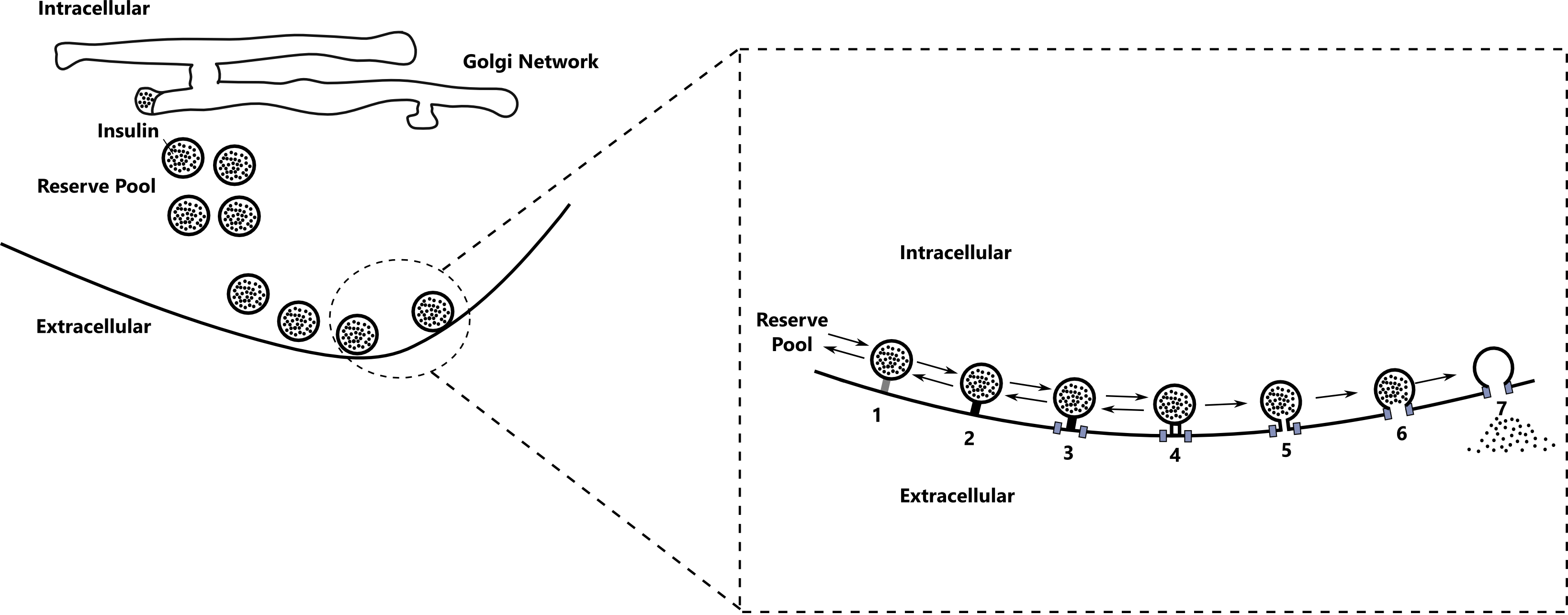
Figure 5: Schematic drawing of exocytosis cascade in $\beta$-cells. On the left, insulin granules produced in Golgi network is transported into extracellular space through exocytosis. On the right, particular steps involved in the exocytosis of the insulin granules. The numbers stand for: 1) Re-supply 2) Priming 3) Domain Binding 4) Ca Triggering 5) Fusion 6) Pore Expansion 7) Insulin Release

Chen et al. [7] developed mathematical model of $\beta$-cell to calculate both rate of granule fusion and the rate of insulin secretion in $\beta$-cells stimulated with electrical potential. The model is based on five-state kinetic model of granule fusion proposed by Voets et al. [31]. Figure 5 illustrates kinetic scheme proposed for exocytosis in pancreatic $\beta$-cells. As it is shown in the figure the model accounts for steps involved in exocytosis cascade such as re-suply, priming, domain binding, Ca²⁺ triggering, fusion, pore expansion and insulin release. It is assumed that L-type (not the R-type) voltage-sensitive Ca²⁺-channels are used for secretion of primed granules through cell membrane. During this process “microdomains” with high Ca²⁺ concentration are formed at the inner mouth of L-type channels (illustrated as circles in Figure 5). Concentration of Ca²⁺ in cytosol and microdomain at time $t$ are denoted by $C_{i}(t)$ and $C_{md}(t)$, respectively. Since the number of granules are far less than number of Ca²⁺, it is also assumed that dynamics of Ca²⁺ is independent of exocytosis cascade. For further details we refer the reader to the original paper [7].

(a) The digraph structure of dynamics presented in [7].

(b) The associated complementary digraph $G^{\star}$ of digraph $G$ illustrated in part a.

(c) Complementary digraph $G^{\star}$ at resting state, when $C_{md}\approx 0$

Figure 6: Exocytosis cascade of insulin granules in pancreatic $\beta$-cells

Figure 6a illustrates the dynamics associated with exocytosis cascade as a digraph $G$. Since complementary digraph of $G$ (Figure 6b) is strongly connected, the steady state solutions of dynamics can be calculated using the algorithm described in Section 3.1. The ES is given as

$$N_{{\scriptscriptstyle ES}}=\Delta\left(\begin{array}[]{c}6k_{-1}^{3}+2u_{1}k_{-1}^{2}+C_{\text{md}}k_{1}u_{1}k_{-1}+2C_{\text{md}}^{2}k_{1}^{2}u_{1}\\ 18C_{\text{md}}k_{1}k_{-1}^{2}+6C_{\text{md}}k_{1}u_{1}k_{-1}+3C_{\text{md}}^{2}k_{1}^{2}u_{1}\\ 18C_{\text{md}}^{2}k_{-1}k_{1}^{2}+6C_{\text{md}}^{2}u_{1}k_{1}^{2}\\ 6C_{\text{md}}^{3}k_{1}^{3}\\ \frac{6r_{-1}k_{-1}^{3}}{r_{1}}+\frac{2r_{-1}u_{1}k_{-1}^{2}}{r_{1}}+\frac{C_{\text{md}}k_{1}r_{-1}u_{1}k_{-1}}{r_{1}}+\frac{6C_{\text{md}}^{3}k_{1}^{3}u_{1}}{r_{1}}+\frac{2C_{\text{md}}^{2}k_{1}^{2}r_{-1}u_{1}}{r_{1}}\\ \frac{6r_{-2}r_{-1}k_{-1}^{3}}{r_{1}r_{2}}+\frac{2r_{-2}r_{-1}u_{1}k_{-1}^{2}}{r_{1}r_{2}}+\frac{C_{\text{md}}k_{1}r_{-2}r_{-1}u_{1}k_{-1}}{r_{1}r_{2}}+\frac{6C_{\text{md}}^{3}k_{1}^{3}u_{1}}{r_{2}}+\frac{6C_{\text{md}}^{3}k_{1}^{3}r_{-2}u_{1}}{r_{1}r_{2}}+\frac{2C_{\text{md}}^{2}k_{1}^{2}r_{-2}r_{-1}u_{1}}{r_{1}r_{2}}\\ \frac{6C_{\text{md}}^{3}k_{1}^{3}u_{1}}{u_{2}}\\ \frac{6C_{\text{md}}^{3}k_{1}^{3}u_{1}}{u_{3}}\end{array}\right)$$

where $\Delta$ is given as follows

$$\begin{array}[]{c}\Delta=\frac{r_{1}r_{2}r_{3}}{r_{-1}r_{-2}r_{-3}\left(\frac{6k_{1}^{3}r_{1}u_{1}C_{\text{md}}^{3}}{r_{-2}r_{-1}}+\frac{6k_{1}^{3}r_{1}r_{2}u_{1}C_{\text{md}}^{3}}{r_{-3}r_{-2}r_{-1}}+\frac{6k_{1}^{3}u_{1}C_{\text{md}}^{3}}{r_{-1}}+k_{1}k_{-1}u_{1}C_{\text{md}}+2k_{1}^{2}u_{1}C_{\text{md}}^{2}+2k_{-1}^{2}u_{1}+6k_{-1}^{3}\right)}\end{array}$$

As we can see the ES gets complicated for the large graphs. However, our framework provides steady state value of any given substrate (see (12)), which is not easily found by numerical simulations.

At the resting state (electric potential set to $V=-70\,mV$ ), concentration of Ca²⁺ in the microdomain is very low, so it is assumed that $C_{md}=C_{md}(t)\approx 0$. In this case, the complementary digraph of $G$ is no longer strongly connected, which is given in Figure 6c. Then the ES solution have to be computed by the process described in Section 3.2.1, and is given as

$$N_{r,{\scriptscriptstyle ES}}=\left(\begin{array}[]{c}\frac{r_{1}r_{2}r_{3}}{r_{-3}r_{-2}r_{-1}}\\ 0\\ 0\\ 0\\ \frac{r_{2}r_{3}}{r_{-3}r_{-2}}\\ \frac{r_{3}}{r_{-3}}\\ 0\\ 0\end{array}\right)$$

In the above example the dynamics were essentially linear. Although the framework in this paper is linear in nature, it can be applied to nonlinear systems as well. This can be done by incorporating nonlinearity into the framework through the edge labels. So far we treated edge weights as uninterpreted symbols. In fact, edge weights can be an arbitrary positive rational expressions. For example, the Michaelis-Menten formula used in enzyme kinetics is a legitimate edge weight

$$a=\frac{V_{max}[S]}{K_{m}+[S]}\,,$$

where $[S]$ stands for the concentration of the substrate $S$, $K_{m}$ and $V_{max}$ are reaction specific constants. However, in most cases a chemical reaction network modeled with mass action kinetics, which gives rise to a nonlinear system of ODEs. The steady states of this type of dynamics can also be algorithmically computed using our framework. For instance, a chemical reaction of type

$$A+B\overset{k}{\longrightarrow}C$$

can be represented in our way as

$$A\overset{kB}{\longrightarrow}C$$

One can then use above formalism to transform chemical reactions into a digraph with time dependent edge weights. Consequently, this digraph can be used to calculate the steady states using our framework. One should keep in mind that in a such transformation only the equilibrium solutions coincide not the transient dynamics [16]. For more extensive discussion of the topic we refer the reader to [16] and [17]. Next we illustrate such incorporation by applying it to a nonlinear biochemical network.

5.2 Glucose metabolism in $\beta$-cells

In their paper Sweet and Matschinsky [29] setup a mathematical model of pancreatic $\beta$-cell glucose metabolism to investigate the relation between glucose and the rate of glycolysis (see Figure 7). Since glucose metabolism in $\beta$-cells indirectly affects the rate of insulin secretion [27], this type of models have implications for the diabetes treatment. All reactions together make dynamics overwhelmingly complex. To avoid this authors assumed that reactions inside dashed rectangles (pools) are operating sufficiently fast, and have reached thermodynamic equilibrium. Then ordinary differential equations are written for the rates of transfers between these pools. Consequently, equilibrium metabolites in a pool are calculated algebraically using equilibrium assumptions. Although the model is minimalistic, it still includes parameters describing overall behavior glycolysis in $\beta$-cell. Nonlinear dynamics associated with the model can be given as in figure 8A. In this case nonlinearity is hidden in label $f$,

$$f=\frac{G_{PK}D\sqrt{b^{2}-b-\frac{8K_{TPI}}{V_{c}}{\scriptstyle GIP(t)}}}{{\scriptstyle GIP(t)}}$$

where ${\scriptstyle GIP(t)}$ stands for concentration of ${\scriptstyle GIP}$ at time $t$, and every other letter are reaction rate constants. Since complementary digraph of $G$ (Figure 8b) is strongly connected, the ES solutions to the system can be obtained by the procedure described in Section 3.1:

$$\left(\begin{array}[]{c}Glu^{*}\\ H-6-P^{*}\\ \frac{1}{2}GIP^{*}\\ Pyr^{*}\end{array}\right)=\frac{1}{bdh+beh+ceh}\left(\begin{array}[]{c}adh+aeh\\ ach\\ \frac{aceh}{f}\\ ace+bdg+beg+ceg\end{array}\right)$$

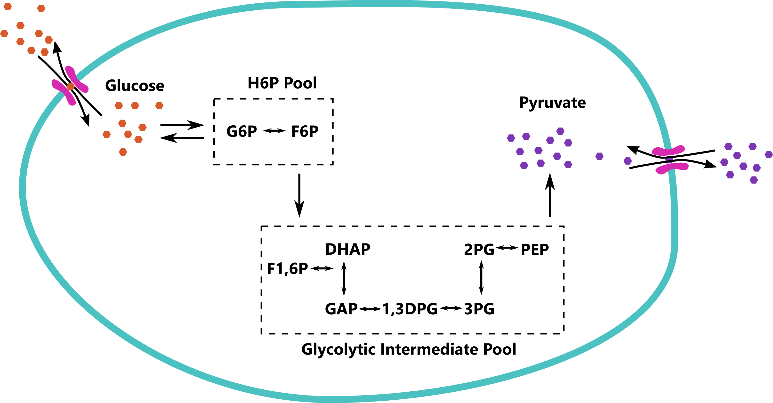
Figure 7: Schematic model of glycolysis in pancreatic $\beta$-cells

(a) The digraph describing the main mechanism of glycolisis

(b) The corresponding complementary digraph $G^{\star}$

Figure 8: Glycolysis in pancreatic $\beta$-cells

6 Conclusions and future work

In our previous work, we have developed a “linear framework” for symbolical computation of equilibrium solutions of Laplacian dynamics, which has applications in many diverse fields of biology such as enzyme kinetics, pharmacology and receptor theory, gene regulation, protein post-translation modification [16, 17, 2]. Our effort here was to extend existing framework for the case when zeroth order synthesis and first order degradation is added to Laplacian dynamics. The main motivation came from [16], where the author discusses the addition of synthesis and degradation to Laplacian dynamics of strongly connected digraph. Here we extended the proposed framework for arbitrary digraph with synthesis and degradation, and showed that synthesis and degradation dynamics possesses unique stable steady state solution under certain necessary and sufficient conditions. These conditions can be also used to identify whether given synthesis and degradation dynamics reaches a steady state. Moreover, as before, we have developed a mathematical framework to compute that unique ES. Our algorithm uses underlying digraph structure of dynamics and computer implementation of previous framework [2] can be revised for automatic computations.

This type of dynamics are frequently encountered in biological literature. In fact, to illustrate utility of our framework we have applied it to several examples in biochemistry such as exocytosis cascade of insulin granules and glucose metabolism in pancreatic $\beta$-cells. Since computed steady states are exact (not an approximation), they can be used to check correctness of numerical solutions. On the other hand, one of the greatest challenges in mathematical modeling is finding required parameters using given set of experimental data. Yet another feature of framework is that it can prove useful in parameter estimation problems. Particularly, one can calibrate computed symbolic ES solutions to experimental results.

Although the latter example, glucose metabolism in $\beta$-cells, demonstrates application of framework to nonlinear system of differential equations, the scope of application of our framework to such nonlinear systems is limited. Therefore, as our future plan we intend to further extend framework such that it can be applied to broader range of nonlinear dynamics.

7 Acknowledgements

Funding for this research was supported in part by grants NIH-NIGMS 2R01GM069438-06A2 and NSF-DMS 1225878. The authors would also like to thank Clay Thompson (Systems Biology Group, Pfizer, Inc.) for his suggestion of the insulin synthesis example used in Section 5.

References

• [1] R P Agaev and P Yu Chebotarev, The Matrix of Maximum Out Forests of a Digraph, 61 (2000), pp. 1424–1450.
• [2] Tobias Ahsendorf, Felix Wong, Roland Eils, and Jeremy Gunawardena, A framework for modelling gene regulation that accommodates non-equilibrium mechanisms, (2013).
• [3] Sebastian Barg, Mechanisms of Exocytosis in Insulin-Secreting B-Cells and, (2003), pp. 3–13.
• [4] D Bérenguier, C Chaouiya, P T Monteiro, A Naldi, E Remy, D Thieffry, and L Tichit, Dynamical modeling and analysis of large cellular regulatory networks., Chaos, 23 (2013), p. 025114.
• [5] Jared C. Bronski and Lee DeVille, Spectral Theory for Dynamics on Graphs Containing Attractive and Repulsive Interactions, SIAM Journal on Applied Mathematics, 74 (2014), pp. 83–105.
• [6] Pavel Chebotarev and Rafig Agaev, Forest matrices around the Laplacian matrix, Linear algebra and its applications, (2002), pp. 1–19.
• [7] Yider Chen, Shaokun Wang, and Arthur Sherman, Identifying the targets of the amplifying pathway for insulin secretion in pancreatic beta-cells by kinetic modeling of granule exocytosis., Biophysical journal, 95 (2008), pp. 2226–41.
• [8] Kuo Chen Chou, Graphic rules in steady and non-steady state enzyme kinetics., Journal of Biological Chemistry, 264 (1989), pp. 12074–12079.
• [9]  , Applications of graph theory to enzyme kinetics and protein folding kinetics. Steady and non-steady-state systems., Biophysical chemistry, 35 (1990), pp. 1–24.
• [10]  , Graphic rule for non-steady-state enzyme kinetics and protein folding kinetics, Journal of Mathematical Chemistry, 12 (1993), pp. 97–108.
• [11] Gheorghe Craciun and Martin Feinberg, Multiple Equilibria in Complex Chemical Reaction Networks: I. The Injectivity Property, SIAM Journal on Applied Mathematics, 65 (2005), pp. 1526–1546.
• [12] Georghe Craciun and Martin Feinberg, Multiple equilibria in complex chemical reaction networks: extensions to entrapped species models, IEE Proceedings - Systems Biology, 153 (2006), p. 179.
• [13] Gheorghe Craciun and Martin Feinberg, Multiple Equilibria in Complex Chemical Reaction Networks: Semiopen Mass Action Systems, SIAM Journal on Applied Mathematics, 70 (2010), pp. 1859–1877.
• [14] Gheorghe Craciun, Yangzhong Tang, and Martin Feinberg, Understanding bistability in complex enzyme-driven reaction networks., Proceedings of the National Academy of Sciences of the United States of America, 103 (2006), pp. 8697–702.
• [15] Mirela Domijan and Markus Kirkilionis, Graph theory and qualitative analysis of reaction networks, Networks and Heterogeneous Media, 3 (2008), pp. 295–322.
• [16] Jeremy Gunawardena, A linear framework for time-scale separation in nonlinear biochemical systems., PloS one, 7 (2012), p. e36321.
• [17]  , Time-scale separation - Michaelis and Menten’s old idea, still bearing fruit., The FEBS journal, 281 (2014), pp. 473–88.
• [18] Edward L. King and Carl Altman, A schematic method of deriving the rate laws for enzyme- catalyzed reactions, (1956).
• [19] G. Kirchhoff, Ueber die Auflösung der Gleichungen, auf welche man bei der Untersuchung der linearen Vertheilung galvanischer Ströme geführt wird, Annalen der Physik und Chemie, 148 (1847), pp. 497–508.
• [20] SX Lin and Jacques Lapointe, Theoretical and experimental biology in one, J. Biomedical Science and Engineering, 2013 (2013), pp. 435–442.
• [21] Sayed-Amir Marashi and Mojtaba Tefagh, A mathematical approach to emergent properties of metabolic networks: partial coupling relations, hyperarcs and flux ratios, Journal of Theoretical Biology, (2014).
• [22] Maya Mincheva, Oscillations in biochemical reaction networks arising from pairs of subnetworks., Bulletin of mathematical biology, 73 (2011), pp. 2277–304.
• [23] Maya Mincheva and Marc R Roussel, Graph-theoretic methods for the analysis of chemical and biochemical networks. I. Multistability and oscillations in ordinary differential equation models., Journal of mathematical biology, 55 (2007), pp. 61–86.
• [24]  , Graph-theoretic methods for the analysis of chemical and biochemical networks. II. Oscillations in networks with delays., Journal of mathematical biology, 55 (2007), pp. 87–104.
• [25] Inomzhon Mirzaev and Jeremy Gunawardena, Laplacian dynamics on general graphs, Bulletin of mathematical biology, (2013).
• [26] Charlotta S Olofsson, Sven O Göpel, Sebastian Barg, Juris Galvanovskis, Xiaosong Ma, Albert Salehi, Patrik Rorsman, and Lena Eliasson, Fast insulin secretion reflects exocytosis of docked granules in mouse pancreatic B-cells., Pflügers Archiv : European journal of physiology, 444 (2002), pp. 43–51.
• [27] Morten Gram Pedersen, Contributions of mathematical modeling of beta cells to the understanding of beta-cell oscillations and insulin secretion., Journal of diabetes science and technology, 3 (2009), pp. 12–20.
• [28] P Rorsman and E Renström, Insulin granule dynamics in pancreatic beta cells., Diabetologia, 46 (2003), pp. 1029–45.
• [29] Ian R. Sweet and Franz M. Matschinsky, Mathematical model of beta-cell glucose metabolism and insulin release. I. Glucokinase as glucosensor hypothesis, American journal of physiology. Endocrinology and metabolism, 268 (1995), pp. E775–E788.
• [30] Takeaki Uno, An algorithm for enumerating all directed spanning trees in a directed graph, no. C, 1996.
• [31] T Voets, E Neher, and T Moser, Mechanisms underlying phasic and sustained secretion in chromaffin cells from mouse adrenal slices., Neuron, 23 (1999), pp. 607–15.
• [32] C B Wollheim and G W Sharp, Regulation of insulin release by calcium., Physiological reviews, 61 (1981), pp. 914–73.