Bayesian Semiparametric Multivariate Density Deconvolution

Abstract

We consider the problem of multivariate density deconvolution when interest lies in estimating the distribution of a vector valued random variable ${\mathbf{X}}$ but precise measurements on ${\mathbf{X}}$ are not available, observations being contaminated by measurement errors ${\mathbf{U}}$. The existing sparse literature on the problem assumes the density of the measurement errors to be completely known. We propose robust Bayesian semiparametric multivariate deconvolution approaches when the measurement error density of ${\mathbf{U}}$ is not known but replicated proxies are available for at least some individuals. Additionally, we allow the variability of ${\mathbf{U}}$ to depend on the associated unobserved values of ${\mathbf{X}}$ through unknown relationships, which also automatically includes the case of multivariate multiplicative measurement errors. Basic properties of finite mixture models, multivariate normal kernels and exchangeable priors are exploited in novel ways to meet modeling and computational challenges. Theoretical results showing the flexibility of the proposed methods in capturing a wide variety of data generating processes are provided. We illustrate the efficiency of the proposed methods in recovering the density of ${\mathbf{X}}$ through simulation experiments. The methodology is applied to estimate the joint consumption pattern of different dietary components from contaminated 24 hour recalls. Supplementary materials present substantive additional details.

Some Key Words: B-splines, Conditional heteroscedasticity, Latent factor analyzers, Measurement errors, Mixture models, Multivariate density deconvolution, Regularization, Shrinkage.

Short Title: Multivariate Density Deconvolution

1 Introduction

Many problems of practical importance require estimation of the density $f_{{\mathbf{X}}}$ of a vector valued random variable ${\mathbf{X}}$. Precise measurements on ${\mathbf{X}}$ may not, however, be available, observations being contaminated by measurement errors ${\mathbf{U}}$. Under the assumption of additive measurement errors, the observations are generated from a convolution of the density $f_{{\mathbf{X}}}$ of ${\mathbf{X}}$ and the density $f_{{\mathbf{U}}}$ of the measurement errors ${\mathbf{U}}$. The problem of estimating the density $f_{{\mathbf{X}}}$ from available contaminated measurements then becomes a problem of multivariate density deconvolution.

This article proposes novel Bayesian semiparametric density deconvolution approaches based on finite mixtures of latent factor analyzers for robust estimation of the density $f_{{\mathbf{X}}}$ when the measurement error density $f_{{\mathbf{U}}}$ is not known, but replicated proxies contaminated with measurement errors ${\mathbf{U}}$ are available for at least some individuals. The proposed deconvolution approaches are highly robust, not having to impose restrictive parametric assumptions on $f_{{\mathbf{X}}}$ or $f_{{\mathbf{U}}}$. Additionally, the variability of ${\mathbf{U}}$ is allowed to depend on the associated unobserved values of ${\mathbf{X}}$ through unknown relationships.

While the focus of the article will primarily be on additive measurement errors, importantly, the methodology for additive conditionally heteroscedastic measurement errors developed here also automatically encompasses the case of multivariate multiplicative measurement errors.

To the best of our knowledge, all existing multivariate deconvolution approaches assume that ${\mathbf{U}}$ is independent of ${\mathbf{X}}$ and that the error density $f_{{\mathbf{U}}}$ is completely known. Ours is thus the first paper that allows the density of the measurement errors to be unknown and free from parametric laws and additionally also accommodates conditional heteroscedasticity in the measurement errors.

The literature on the problem of univariate density deconvolution, in which context we denote the variable of interest by $X$ and the measurement errors by $U$, is vast. Most of the early literature considered scenarios when the measurement error density $f_{U}$ is completely known. Fourier inversion based deconvoluting kernel density estimators have been studied by Carroll and Hall (1988), Liu and Taylor (1989), Devroye (1989), Fan (1991a, 1991b, 1992) and Hesse (1999) among many others. For a review of these methods, the reader may be referred to Section 12.1 in Carroll, et al. (2006) and Section 10.2.3 in Buonaccorsi (2010). In reality $f_{U}$ is rarely known. The problem of deconvolution when the errors are homoscedastic with an unknown density and replicated proxies are available for each subject has been addressed by Li and Vuong (1998). See also Diggle and Hall (1993), Neumann (1997), Carroll and Hall (2004) and the references therein. The assumptions of homoscedasticity of $U$ and their independence from $X$ are also often unrealistic. Flexible Bayesian density deconvolution approaches that allow $U$ to be conditionally heteroscedastic have recently been developed in Staudenmayer, et al. (2008) and Sarkar, et al. (2014). Staudenmayer, et al. (2008) assumed the measurement errors to be normally distributed and used finite mixtures of B-splines to estimate $f_{X}$ and a variance function that captured the conditional heteroscedasticity. Sarkar, et al. (2014) further relaxed the assumption of normality of $U$ employing flexible infinite mixtures of normal kernels induced by Dirichlet processes to estimate both $f_{X}$ and $f_{U}$. Sieve based methods developed in Schennach (2004) and Hu and Schennach (2008) can also handle conditional heteroscedasticity.

In sharp contrast to the univariate case, the literature on multivariate density deconvolution is quite sparse. We can only mention Masry (1991), Youndjé and Wells (2008), Comte and Lacour (2013), Hazelton and Turlach (2009, 2010) and Bovy, et al. (2011). The first three considered deconvoluting kernel based approaches assuming the measurement errors ${\mathbf{U}}$ to be distributed independently from ${\mathbf{X}}$ according to a known probability law. Hazelton and Turlach (2009, 2011), working with the same assumptions on ${\mathbf{U}}$, proposed weighted kernel based methods. Bovy, et al. (2011) modeled the density $f_{{\mathbf{X}}}$ using flexible mixtures of multivariate normal kernels, but they assumed $f_{{\mathbf{U}}}$ to be multivariate normal with known covariance matrices, independent from ${\mathbf{X}}$. As in the case of univariate problems, the assumptions of a fully specified $f_{{\mathbf{U}}}$, known covariance matrices, and independence from ${\mathbf{X}}$ are highly restrictive for most practical applications.

The focus of this article is on multivariate density deconvolution when $f_{{\mathbf{U}}}$ is not known but replicated proxies are available for at least some individuals. The proposed deconvolution approaches can additionally accommodate conditional heteroscedasticity in ${\mathbf{U}}$. The problem is important, for instance, in nutritional epidemiology, where nutritionists are typically interested not just in the consumption behaviors of individual dietary components but also in their joint consumption patterns. The data are often available in the form of dietary recalls and are contaminated by measurement errors that show strong patterns of conditional heteroscedasticity.

As in Sarkar, et al. (2014), we use mixture models to estimate both $f_{{\mathbf{X}}}$ and $f_{{\mathbf{U}}}$ but the multivariate nature of the problem brings in new modeling challenges and computational obstacles that preclude straightforward extension of their univariate deconvolution approaches. Instead of using infinite mixtures induced by Dirichlet processes, we use finite mixtures of multivariate normal kernels with exchangeable Dirichlet priors on the mixture probabilities. The use of finite mixtures and exchangeable priors greatly reduces computational complexity while retaining essentially the same flexibility. Carefully constructed priors also allow automatic model selection and model averaging. To save space, detailed discussions on these important issues are moved to Section S.6 in the Supplementary Materials.

We also exploit symmetric Dirichlet priors and properties of multivariate normal distributions and finite mixture models to develop a novel strategy that enables us to enforce a required zero mean restriction on the measurement errors. Our proposed technique, as opposed to the one adopted by Sarkar, et al. (2014), is particularly suitable for high dimensional applications and can be easily generalized to enforce moment restrictions on other types of finite mixture models.

It is well known that inverse Wishart priors, due to their dense parametrization, are not suitable for modeling covariance matrices in high dimensional applications. In deconvolution problems the issue is further complicated since ${\mathbf{X}}$ and ${\mathbf{U}}$ are both latent. This results in numerically unstable estimates even for small and moderate dimensions, particularly when the true covariance matrices are sparse and the likelihood function is of complicated form. To reduce the effective number of parameters required to be estimated, we consider factor-analytic representation of the component specific covariance matrices with sparsity inducing shrinkage priors on the factor loading matrices.

Models for multivariate regression errors that assume normality but allow the covariance matrix to vary flexibly with associated precisely measured and possibly multivariate predictors have recently been developed in the literature (Hoff and Niu, 2012; Fox and Dunson, 2016, etc.). Unlike regression settings, exclusive relationships exist between different components of multivariate measurement errors ${\mathbf{U}}$ and different components of the associated multivariate latent ‘predictor’ ${\mathbf{X}}$ - the $\ell^{th}$ component $U_{\ell}$ of ${\mathbf{U}}$ contaminates only the $\ell^{th}$ component $X_{\ell}$ of ${\mathbf{X}}$ but not others. We thus deem covariance regression models that allow $\hbox{cov}({\mathbf{U}}|{\mathbf{X}})$ to vary arbitrarily with all components of ${\mathbf{X}}$ to be inappropriate in multivariate measurement error settings. As discussed above, the assumption of multivariate normality is also particularly restrictive in measurement error problems. In this article, we develop a semiparametric approach that appropriately highlights the exclusive associations between $U_{\ell}$ and $X_{\ell}$ while allowing the distribution of $({\mathbf{U}}|{\mathbf{X}})$ to depart from normality. Importantly, the model also arises naturally from multivariate multiplicative measurement error settings, automatically encompassing such cases. Diagnostic tools for checking model adequacy are also discussed.

The likelihood function for the conditional heteroscedastic model poses significant computational challenges. We overcome these obstacles by designing a novel two-stage procedure that exploits the unique properties of conditionally heteroscedastic multivariate measurement errors to our advantage. The procedure first estimates the variance functions characterizing $\hbox{var}(U_{\ell}|X_{\ell})$ using reparametrized versions of the corresponding univariate submodels. The estimates obtained in the first stage are then plugged-in to estimate the remaining parameters in the second stage. Having two estimation stages, our deconvolution method for conditionally heteroscedastic measurement errors is not purely Bayesian. But they show good empirical performance and, with no other solution available in the existing literature, they provide at least workable starting points towards more sophisticated methodology.

The article is organized as follows. Section 2 details the models. Model identifiability issues and implementation details, including the choice of hyper-parameters and Markov chain Monte Carlo (MCMC) algorithms to sample from the posterior, are discussed in the Supplementary Materials. Section 4 discusses model identifiability issues. Section 5 presents theoretical results showing flexibility of the proposed models. Simulation studies comparing the proposed deconvolution methods to a naive method that ignores measurement errors are presented in Section 6. Section 7 presents an application of the proposed methodology in estimation of the joint consumption pattern of dietary intakes from contaminated 24 hour recalls in a nutritional epidemiologic study. Section 8 includes a discussion. An unnumbered section concludes the article with a description of the Supplementary Materials.

2 Deconvolution Models

The goal is to estimate the unknown joint density of a $p$-dimensional multivariate random variable ${\mathbf{X}}$. There are $i=1,\dots,n$ subjects. Precise measurements of ${\mathbf{X}}$ are not available. Instead, for $j=1,\dots,m_{i}$, replicated proxies ${\mathbf{W}}_{ij}$ contaminated with measurement errors ${\mathbf{U}}_{ij}$ are available for each subject $i$. The replicates are assumed to be generated by the model

$${\mathbf{W}}_{ij} = {\mathbf{X}}_{i}+{\mathbf{U}}_{ij}.$$ (1)

Given ${\mathbf{X}}_{i}$, ${\mathbf{U}}_{ij}$ are independently distributed with $E({\mathbf{U}}_{ij}|{\mathbf{X}}_{i})={\mathbf{0}}$. The marginal density of ${\mathbf{W}}_{ij}$ is denoted by $f_{{\mathbf{W}}}$. The implied conditional distributions of ${\mathbf{W}}_{ij}$ and ${\mathbf{U}}_{ij}$, given ${\mathbf{X}}_{i}$, are denoted by $f_{{\mathbf{W}}|{\mathbf{X}}}$ and $f_{{\mathbf{U}}|{\mathbf{X}}}$, respectively.

2.1 Modeling the Density $f_{{\mathbf{X}}}$

In this article $f_{{\mathbf{X}}}$ is specified as a mixture of multivariate normal kernels

$$f_{{\mathbf{X}}}({\mathbf{X}})=\textstyle\sum_{k=1}^{K_{{\mathbf{X}}}}\pi_{{\mathbf{X}},k}~{}\hbox{MVN}_{p}({\mathbf{X}}|\mbox{\boldmath$\mu$}_{{\mathbf{X}},k},\mbox{\boldmath$\Sigma$}_{{\mathbf{X}},k}),$$ (2)

where $\hbox{MVN}_{p}(\cdot|\mbox{\boldmath$\mu$},\mbox{\boldmath$\Sigma$})$ denotes a $p$-dimensional multivariate normal density with mean $\mu$ and covariance matrix $\Sigma$. For the rest of this subsection, the subscript ${\mathbf{X}}$ is kept implicit to keep the notation clean.

We assign a finite Dirichlet prior to the mixture probability vector $\mbox{\boldmath$\pi$}=(\pi_{1},\dots,\pi_{K})^{\rm T}$ as

$$\pi \sim \hbox{Dir}(\alpha/K,\dots,\alpha/K).$$ (3)

Here $\hbox{Dir}(\alpha_{1},\dots,\alpha_{K})$ denotes a finite dimensional Dirichlet distribution on the $K$-dimensional unit simplex with concentration parameter $(\alpha_{1},\dots,\alpha_{K})$. Given $K$ and the latent cluster membership indices, the prior is conjugate. The symmetry of the assumed Dirichlet prior helps in additional reduction of computational complexity by simplifying MCMC mixing issues. Provided $K$ is sufficiently large, a carefully chosen $\alpha$ can impart the posterior with certain properties that simplify model selection and model averaging issues by influencing the posterior to concentrate in regions that favor empty redundant components, see Section S.1 and Section S.6 of the Supplementary Materials. We assign conjugate multivariate normal priors to the component specific mean vectors $\mbox{\boldmath$\mu$}_{k}$, so that

$$\mbox{\boldmath$\mu$}_{k} \sim \hbox{MVN}_{p}(\mbox{\boldmath$\mu$}_{0},\mbox{\boldmath$\Sigma$}_{0}).$$ (4)

The conjugacy again helps in simplifying posterior calculations. Later on, we will employ similar mixture models for the density of the measurement errors, and this conjugacy, along with some basic properties of multivariate normal kernels, will also help us enforce the mean zero restriction on the measurement errors. For the component specific covariance matrices $\mbox{\boldmath$\Sigma$}_{k}$, we first consider conjugate inverse Wishart priors

$$\ \mbox{\boldmath$\Sigma$}_{k}\sim\hbox{IW}_{p}(\nu_{0},\mbox{\boldmath$\Psi$}_{0}).$$ (5)

Here $\hbox{IW}_{p}(\nu,\mbox{\boldmath$\Psi$})$ denotes an inverse Wishart density on the space of $p\times p$ positive definite matrices with mean $\mbox{\boldmath$\Psi$}/(\nu-p-1)$. While the conjugacy of the inverse Wishart priors helps in simplifying posterior calculations, in complex high dimensional problems its dense parameterization may result in numerically unstable estimates, particularly when the covariance matrices are sparse. In a deconvolution problem the issue is compounded further by the nonavailability of the true ${\mathbf{X}}_{i}$’s. To reduce the effective number of parameters to be estimated, we consider a parsimonious factor-analytic representation of the component specific covariance matrices:

$$\mbox{\boldmath$\Sigma$}_{k}=\mbox{\boldmath$\Lambda$}_{k}\mbox{\boldmath$\Lambda$}_{k}^{\rm T}+\mbox{\boldmath$\Omega$},$$ (6)

where $\mbox{\boldmath$\Lambda$}_{k}$ are $p\times q_{k}$ factor loading matrices and $\Omega$ is a diagonal matrix with non-negative entries. In practical applications $q_{k}$ will typically be much smaller than $p$, inducing parsimonious characterizations of the unknown covariance matrices $\mbox{\boldmath$\Sigma$}_{k}$. Model (2) can be equivalently represented as

$$\Pr(C_{i}=k)=\pi_{k},$$ (7)

$$({\mathbf{X}}_{i}|C_{i}=k)=\mbox{\boldmath$\mu$}_{k}+\mbox{\boldmath$\Lambda$}_{k}\mbox{\boldmath$\eta$}_{i}+\mbox{\boldmath$\Delta$}_{i},$$ (8)

$$\mbox{\boldmath$\eta$}_{i}\sim\hbox{MVN}_{p}({\mathbf{0}},{\mathbf{I}}_{p}),~{}~{}~{}~{}~{}\mbox{\boldmath$\Delta$}_{i}\sim\hbox{MVN}_{p}({\mathbf{0}},\mbox{\boldmath$\Omega$}),$$ (9)

where $C_{i}$ are the mixture labels associated with ${\mathbf{X}}_{i}$, $\mbox{\boldmath$\eta$}_{i}$ are latent factors, and $\mbox{\boldmath$\Delta$}_{i}$ are errors with covariance $\mbox{\boldmath$\Omega$}=\hbox{diag}(\sigma_{1}^{2},\dots,\sigma_{p}^{2})$.

The above characterization of $\mbox{\boldmath$\Sigma$}_{k}$ is not unique, since for any semi-orthogonal matrix ${\mathbf{P}}$ the loading matrix $\mbox{\boldmath$\Lambda$}_{k}^{1}=\mbox{\boldmath$\Lambda$}_{k}{\mathbf{P}}$ also satisfies (6). Since interest lies primarily in estimating the density $f_{{\mathbf{X}}}$, identifiability of the latent factors is, however, not required. This also allows the loading matrices to have a-priori a potentially infinite number of columns. Sparsity inducing priors, that favor more shrinkage as the column index increases, can then be used to shrink the redundant columns towards zero. In this article, we do this by adapting the shrinkage priors proposed in Bhattacharya and Dunson (2011) that allow easy posterior computation. Let $\mbox{\boldmath$\Lambda$}_{k}=((\lambda_{k,jh}))_{j=1,h=1}^{p,\infty}$, where $j$ and $h$ denote the row and the column indices, respectively. For $h=1,\dots,\infty$, we assign priors as follows

$$\lambda_{k,jh} \sim \hbox{Normal}(0,\phi_{k,jh}^{-1}\tau_{k,h}^{-1}),~{}~{}~{}~{}~{}\phi_{k,jh}\sim\hbox{Ga}(\nu/2,\nu/2),$$ (10)

$$\tau_{k,h} \sim \textstyle\prod_{\ell=1}^{h}\delta_{k,\ell},~{}~{}~{}~{}~{}\delta_{k,\ell}\sim\hbox{Ga}(a_{\ell},1),~{}~{}~{}~{}~{}\sigma_{j}^{2}\sim\hbox{Inv-Ga}(a_{\sigma},b_{\sigma}).$$ (11)

Here $\hbox{Ga}(\alpha,\beta)$ denotes a Gamma distribution with shape parameter $\alpha$ and rate parameter $\beta$ and $\hbox{IG}(a,b)$ denotes an inverse-Gamma distribution with shape parameter $a$ and scale parameter $b$. In the $k^{th}$ component factor loading matrix $\mbox{\boldmath$\Lambda$}_{k}$, the parameters $\{\phi_{k,jh}\}_{j=1}^{p}$ control the local shrinkage of the elements in the $h^{th}$ column, whereas $\tau_{k,h}$ controls the global shrinkage. When $a_{h}>1$ for $h=2,\dots,\infty$, the sequence $\{\tau_{k,h}\}_{h=1}^{\infty}$ becomes stochastically increasing and thus favors more shrinkage as the column index $h$ increases.

In addition to inducing adaptive sparsity and hence numerical stability, by favoring more shrinkage as the column index increases, the shrinkage priors play another important role in making the proposed factor analytic model highly robust to misspecification of the number of latent factors, allowing us to adopt simple strategies to determine the number of latent factors to be included in the model in practice. Details are deferred to Section S.1.

Throughout the rest of the paper, mixtures with inverse Wishart prior on the covariance matrices will be referred to as MIW models and mixtures of latent factor analyzers will be referred to as MLFA models.

For a review of finite mixture models and mixtures of latent factor analyzers, without moment restrictions or sparsity inducing priors and with applications in measurement error free scenarios, see Fokoué and Titterington (2003), Frühwirth-Schnatter (2006), Mengersen, et al. (2011) and the references therein. For other types of shrinkage priors, see Brown and Griffin (2010), Carvalho, et al. (2010), Bhattacharya, et al. (2014) etc.

2.2 Modeling the Density of the Measurement Errors

2.2.1 Independently Distributed Measurement Errors

In this section, we develop models for the measurement errors ${\mathbf{U}}$ assuming them to be independent from ${\mathbf{X}}$. That is, we assume $f_{{\mathbf{U}}|{\mathbf{X}}}=f_{{\mathbf{U}}}$ for all ${\mathbf{X}}$. This remains the most extensively researched deconvolution problem for both univariate and multivariate cases. The techniques developed in this section will also provide crucial building blocks for more realistic models in Section 2.2.2. The measurement errors and their density are now denoted by $\mbox{\boldmath$\epsilon$}_{ij}$ and $f_{\mbox{\boldmath$\epsilon$}}$, respectively, for reasons to become obvious shortly in Section 2.2.2.

As in Section 2.1, a mixture of multivariate normals can be used to model the density $f_{\mbox{\boldmath$\epsilon$}}$ but the model now has to satisfy a mean zero constraint. That is

$$f_{\mbox{\boldmath$\epsilon$}}(\mbox{\boldmath$\epsilon$})=\textstyle\sum_{k=1}^{K_{\mbox{\boldmath$\epsilon$}}}\pi_{\mbox{\boldmath$\epsilon$},k}~{}\hbox{MVN}_{p}(\mbox{\boldmath$\epsilon$}|\mbox{\boldmath$\mu$}_{\mbox{\boldmath$\epsilon$},k},\mbox{\boldmath$\Sigma$}_{\mbox{\boldmath$\epsilon$},k}),$$ (12)

$$\text{subject to}~{}\textstyle\sum_{k=1}^{K_{\mbox{\boldmath$\epsilon$}}}\pi_{\mbox{\boldmath$\epsilon$},k}\mbox{\boldmath$\mu$}_{\mbox{\boldmath$\epsilon$},k}={\mathbf{0}}.$$ (13)

To get numerically stable estimates of the density of the errors, latent factor characterization of the covariance matrices with sparsity inducing shrinkage priors as in Section 2.1 may again be used. Details are curtailed to avoid unnecessary repetition and we only present the mechanism to enforce the zero mean restriction on the model. The subscript $\epsilon$ is again dropped in favor of cleaner notation. In later sections, the subscripts ${\mathbf{X}}$ and $\epsilon$ reappear to distinguish between the parameters associated with $f_{{\mathbf{X}}}$ and $f_{\mbox{\boldmath$\epsilon$}}$, when necessary.

Without the mean restriction and under conjugate multivariate normal priors $\mbox{\boldmath$\mu$}_{k}\sim\hbox{MVN}_{p}(\mbox{\boldmath$\mu$}_{0},\mbox{\boldmath$\Sigma$}_{0})$, the posterior full conditional of $\mbox{\boldmath$\mu$}^{Kp\times 1}=(\mbox{\boldmath$\mu$}_{1}^{\rm T},\dots,\mbox{\boldmath$\mu$}_{K}^{\rm T})^{\rm T}$ is given by

$$\hbox{MVN}_{Kp}\left\{\left(\begin{array}[]{c}\mbox{\boldmath$\mu$}_{1}^{0}\\ \mbox{\boldmath$\mu$}_{2}^{0}\\ \vdots\\ \mbox{\boldmath$\mu$}_{K}^{0}\end{array}\right),\left(\begin{array}[]{c c c c}\mbox{\boldmath$\Sigma$}_{1}^{0}&{\mathbf{0}}&\dots&{\mathbf{0}}\\ {\mathbf{0}}&\mbox{\boldmath$\Sigma$}_{2}^{0}&\dots&{\mathbf{0}}\\ \vdots&\vdots&&\vdots\\ {\mathbf{0}}&{\mathbf{0}}&\dots&\mbox{\boldmath$\Sigma$}_{K}^{0}\end{array}\right)\right\}\equiv\hbox{MVN}_{Kp}(\mbox{\boldmath$\mu$}^{0},\mbox{\boldmath$\Sigma$}^{0}),$$ (22)

where $\mbox{\boldmath$\epsilon$}_{ij}$ and other conditioning variables are implicitly understood. Explicit expressions of $\mbox{\boldmath$\mu$}^{0}$ and $\mbox{\boldmath$\Sigma$}^{0}$ in terms of the conditioning variables can be found in Section S.1. The posterior full conditional of $\mu$ under the mean restriction can then be obtained easily by further conditioning the distribution in (22) by $\mbox{\boldmath$\mu$}_{R}=\sum_{k=1}^{K}\pi_{k}\mbox{\boldmath$\mu$}_{k}=0$ and is given by

$$(\mbox{\boldmath$\mu$}|\mbox{\boldmath$\mu$}_{R}={\mathbf{0}})\sim\hbox{MVN}_{Kp}\{\mbox{\boldmath$\mu$}^{0}-\mbox{\boldmath$\Sigma$}_{1,R}^{0}(\mbox{\boldmath$\Sigma$}_{R,R}^{0})^{-1}\mbox{\boldmath$\mu$}_{R}^{0},\mbox{\boldmath$\Sigma$}^{0}-\mbox{\boldmath$\Sigma$}_{1,R}^{0}(\mbox{\boldmath$\Sigma$}_{R,R}^{0})^{-1}\mbox{\boldmath$\Sigma$}_{R,1}^{0}\},$$ (23)

where $\mbox{\boldmath$\mu$}_{R}^{0}=\sum_{k=1}^{K}\pi_{k}\mbox{\boldmath$\mu$}_{k}^{0}=E(\mbox{\boldmath$\mu$}_{R})$, $\mbox{\boldmath$\Sigma$}_{k,K}=\pi_{k}\mbox{\boldmath$\Sigma$}_{k}^{0}=\hbox{cov}(\mbox{\boldmath$\mu$}_{k},\mbox{\boldmath$\mu$}_{R})$, $\mbox{\boldmath$\Sigma$}_{R,R}^{0}=\mbox{\boldmath$\Sigma$}_{K+1,K+1}=\sum_{k=1}^{K}\pi_{k}^{2}\mbox{\boldmath$\Sigma$}_{k}^{0}=\hbox{cov}(\mbox{\boldmath$\mu$}_{R})$, and $\mbox{\boldmath$\Sigma$}_{R,1}^{0}=(\mbox{\boldmath$\Sigma$}_{1,K+1},\mbox{\boldmath$\Sigma$}_{2,K+1},\dots,\mbox{\boldmath$\Sigma$}_{K,K+1})$. To sample from this singular density, we can first sample from the non-singular distribution of $\{(\mbox{\boldmath$\mu$}_{1}^{\rm T},\mbox{\boldmath$\mu$}_{2}^{\rm T},\dots,\mbox{\boldmath$\mu$}_{K-1}^{\rm T})^{\rm T}|\mbox{\boldmath$\mu$}_{R}={\mathbf{0}}\}$, which can also be trivially obtained from (23), and then set $\mbox{\boldmath$\mu$}_{K}=-\sum_{k=1}^{K-1}\pi_{k}\mbox{\boldmath$\mu$}_{k}/\pi_{K}$.

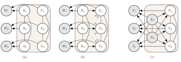
Figure 1: Dependency structures in trivariate deconvolution problems with (a) independently distributed and (b) conditionally varying measurement errors. (c) Dependency structure in a trivariate regression problem with response ${\mathbf{Y}}$, regression errors ${\mathbf{U}}$ and bivariate predictor ${\mathbf{X}}$. The filled rectangular regions focus on the relationship between the (potentially conditionally varying) errors ${\mathbf{U}}$ and the (corresponding conditioning) variable ${\mathbf{X}}$. The unfilled and the shaded nodes signify latent and observable variables, respectively. The directed and the undirected edges represent one and two-way relationships, respectively. The solid black and the dashed gray edges in panel (b) signify strong and weak dependencies, respectively.

2.2.2 Conditionally Heteroscedastic Measurement Errors

We now consider the case when the variances of the measurement errors depend on the associated unknown values of ${\mathbf{X}}$ through unknown relationships.

Interpreting the conditioning variables ${\mathbf{X}}$ broadly as predictors, one can loosely connect our problem of modeling conditionally heteroscedastic ${\mathbf{U}}$ to the problem of covariance regression (Hoff and Niu, 2012; Fox and Dunson, 2016, etc.), where the covariance of the multivariate regression errors are allowed to vary flexibly with precisely measured and possibly multivariate predictors. In such problems, the dimension of the regression errors is unrelated to the dimension of the predictors and different components of the regression errors are assumed to be equally influenced by different components of the predictors. In multivariate deconvolution problems, in contrast, the dimension of ${\mathbf{U}}_{ij}$ is exactly the same as the dimension of ${\mathbf{X}}_{i}$, the $\ell^{th}$ component $U_{ij\ell}$ being the measurement error associated exclusively with $X_{i\ell}$. See Figure 1. While different components of ${\mathbf{U}}_{ij}$ may be correlated, this exclusive association between $U_{ij\ell}$ and $X_{i\ell}$ implies that the dependence of $U_{ij\ell}$ on ${\mathbf{X}}_{i}$ should be explained primarily through $X_{i\ell}$. Figure 7, for instance, suggests strong conditional heteroscedasticity patterns and it is plausible to assume that this conditional variability in $U_{ij\ell}$ can be explained mostly through $X_{i\ell}$ only. It is interesting to note these contrasts between conditionally varying regression and measurement errors become particularly prominent in the multivariate set up. Additionally, the aforementioned covariance regression approaches all assume multivariate normality of the regression errors. As discussed in the introduction, such strong parametric assumptions on the error distribution are particularly restrictive in measurement error problems. Additional detailed discussions of these important issues and resulting modeling implications can be found in Section S.5 of the Supplementary Materials. They preclude direct application of existing covariance regression approaches to multivariate deconvolution problems but warrant models that can highlight the aforementioned unique dependence relationships, accommodate distributional flexibility while enforcing the mean zero restriction, and produce computationally stable estimates even in the absence of precise information on the conditioning variable ${\mathbf{X}}$.

The semiparametric approach that we adopt in this article achieves distributional flexibility, enforces the mean zero restriction, accommodates the exclusive relationships between $U_{ij\ell}$ and $X_{i\ell}$ but ignores the weak dependencies of $U_{ij\ell}$ on $\{X_{im}\}_{m\neq\ell}$ depicted in Figure 1(b). Specifically, we let

$$({\mathbf{U}}_{ij}|{\mathbf{X}}_{i})={\mathbf{S}}({\mathbf{X}}_{i})\mbox{\boldmath$\epsilon$}_{ij},$$ (24)

where ${\mathbf{S}}({\mathbf{X}}_{i})=\hbox{diag}\{s_{1}(X_{i1}),s_{2}(X_{i2}),\dots,s_{p}(X_{ip})\}$ and $\mbox{\boldmath$\epsilon$}_{ij}$, henceforth referred to as the ‘scaled errors’, are distributed independently of ${\mathbf{X}}_{i}$. Model (24) implies that $\hbox{cov}({\mathbf{U}}_{ij}|{\mathbf{X}}_{i})={\mathbf{S}}({\mathbf{X}}_{i})~{}\hbox{cov}(\mbox{\boldmath$\epsilon$}_{ij})~{}{\mathbf{S}}({\mathbf{X}}_{i})$ and marginally $\hbox{var}(U_{ij\ell}|{\mathbf{X}}_{i})=s_{\ell}^{2}(X_{i\ell})\hbox{var}(\epsilon_{ij\ell})$, a function of $X_{i\ell}$ only. The techniques developed in Section 2.2.1 can now be employed to model the density of $\mbox{\boldmath$\epsilon$}_{ij}$, allowing different components of ${\mathbf{U}}_{ij}$ to be correlated and their joint density to deviate from multivariate normality.

We model the variance functions $s_{\ell}^{2}$, denoted also by $v_{\ell}$, using positive mixtures of B-spline basis functions with smoothness inducing priors on the coefficients as in Staudenmayer, et al. (2008). For the $\ell^{th}$ component, partition an interval $[A_{\ell},B_{\ell}]$ of interest into $L_{\ell}$ subintervals using knot points $A_{\ell}=t_{\ell,1}=\dots=t_{\ell,q+1}<t_{\ell,q+2}<t_{\ell,q+3}<\dots<t_{\ell,q+L_{k}}<t_{\ell,q+L_{\ell}+1}=\dots=t_{\ell,2q+L_{\ell}+1}=B_{\ell}$. A flexible model for the variance functions is given by

$$v_{\ell}(X_{i\ell})=s_{\ell}^{2}(X_{i\ell})=\textstyle\sum_{j=1}^{J_{\ell}}b_{q,j,\ell}(X_{i\ell})\exp(\xi_{j\ell})={\mathbf{B}}_{q,J_{\ell},\ell}(X_{i\ell})\exp(\mbox{\boldmath$\xi$}_{\ell}),$$ (25)

$$(\mbox{\boldmath$\xi$}_{\ell}|J_{\ell},\sigma_{\xi,\ell}^{2})\propto(2\pi\sigma_{\xi,\ell}^{2})^{-J_{\ell}/2}\exp\{-\mbox{\boldmath$\xi$}_{\ell}^{\rm T}P_{\ell}\mbox{\boldmath$\xi$}_{\ell}/(2\sigma_{\xi,\ell}^{2})\},~{}~{}~{}~{}\sigma_{\xi,\ell}^{2}\sim\hbox{Inv-Ga}(a_{\xi},b_{\xi}).$$ (26)

Here $\{b_{q,j,\ell}\}_{j=1}^{J_{\ell}}$ denote $J_{\ell}=(q+L_{\ell})$ B-spline bases of degree $q$ as defined in de Boor (2000), $\mbox{\boldmath$\xi$}_{\ell}=\{\xi_{1\ell},\xi_{2\ell},\dots,\xi_{J_{\ell}\ell}\}^{\rm T}$; $\exp(\mbox{\boldmath$\xi$}_{\ell})=\{\exp(\xi_{1\ell}),\exp(\xi_{2\ell}),\dots,\exp(\xi_{J_{\ell}\ell})\}^{\rm T}$; and $P_{\ell}=D_{\ell}^{\rm T}D_{\ell}$, where $D_{\ell}$ is a $J_{\ell}\times(J_{\ell}+2)$ matrix such that $D_{\ell}\mbox{\boldmath$\xi$}_{\ell}$ computes the second differences in $\mbox{\boldmath$\xi$}_{\ell}$. The prior $P_{0}(\mbox{\boldmath$\xi$}_{\ell}|\sigma_{\xi,\ell}^{2})$ induces smoothness in the coefficients because it penalizes $\sum_{j=1}^{J_{k}}(\Delta^{2}\xi_{j\ell})^{2}=\mbox{\boldmath$\xi$}_{\ell}^{\rm T}P_{\ell}\mbox{\boldmath$\xi$}_{\ell}$, the sum of squares of the second order differences in $\mbox{\boldmath$\xi$}_{\ell}$ (Eilers and Marx, 1996). The parameters $\sigma_{\xi,\ell}^{2}$ play the role of smoothing parameter - the smaller the value of $\sigma_{\xi,\ell}^{2}$, the stronger the penalty and the smoother the variance function. The inverse-Gamma hyper-priors on $\sigma_{\xi,\ell}^{2}$ allow the data to have influence on the posterior smoothness and make the approach data adaptive.

Since $s_{\ell}^{2}(X_{i\ell})\hbox{var}(\epsilon_{ij\ell})=\{s_{\ell}^{2}(X_{i\ell})c\}\{\hbox{var}(\epsilon_{ij\ell})/c\}$ for any $c>0$, the variance functions $s_{\ell}^{2}$’s can not be uniquely determined without additional restrictions on $\hbox{var}(\epsilon_{ij\ell})$. Separate identifiability of ${\mathbf{S}}$ and $f_{\mbox{\boldmath$\epsilon$}}$ is, however, not required for inference on $f_{{\mathbf{X}}}$ or to assess the conditional variability in $U_{ij\ell}$. The latter, for instance, may simply be obtained as $\hbox{var}(U_{ij\ell}|X_{i})=s_{\ell}^{2}(X_{i\ell})\hbox{var}(\epsilon_{ij\ell})$. We thus avoid additional identifiability restrictions that would further compound modeling challenges. Adjustments made to the estimates of $s_{\ell}^{2}$ and $f_{\mbox{\boldmath$\epsilon$}}$ to enable comparisons with the corresponding true values in simulation experiments are discussed in Section S.3 in the Supplementary Materials.

2.2.3 Multiplicative Measurement Errors

In this section we consider the case of multivariate multiplicative measurement errors. The replicates are now assumed to be generated by the model

$${\mathbf{W}}_{ij} = {\mathbf{X}}_{i}\circ\widetilde{\mathbf{U}}_{ij},$$ (27)

where $\circ$ denotes element wise product and the errors $\widetilde{\mathbf{U}}_{ij}$ are distributed independently of ${\mathbf{X}}_{i}$ with $E(\widetilde{\mathbf{U}}_{ij})={\mathbf{1}}$. Importantly, model (27) can be reformulated to arrive at model (24) as

$${\mathbf{W}}_{ij} = {\mathbf{X}}_{i}\circ\widetilde{\mathbf{U}}_{ij}={\mathbf{X}}_{i}+{\mathbf{U}}_{ij},~{}~{}~{}\text{with}~{}~{}~{}{\mathbf{U}}_{ij}={\mathbf{X}}_{i}\circ(\widetilde{\mathbf{U}}_{ij}-{\mathbf{1}})={\mathbf{S}}({\mathbf{X}}_{i})\mbox{\boldmath$\epsilon$}_{ij}.$$ (28)

with $E({\mathbf{U}}_{ij}|{\mathbf{X}}_{i})={\mathbf{X}}_{i}\circ E(\widetilde{\mathbf{U}}_{ij}-{\mathbf{1}})={\mathbf{0}}$, ${\mathbf{S}}({\mathbf{X}}_{i})=\hbox{diag}\{s_{1}(X_{i1}),\dots,s_{p}(X_{ip})\}$ with $s_{\ell}(X_{i\ell})=X_{i\ell}$ and $\mbox{\boldmath$\epsilon$}_{ij}=(\widetilde{\mathbf{U}}_{ij}-1)$ are independent of ${\mathbf{X}}_{i}$ with $E(\mbox{\boldmath$\epsilon$}_{ij})={\mathbf{0}}$. This observation precludes the need for separate methodology to be developed for the problem of multivariate density deconvolution in the presence of multiplicative measurement errors and further emphasizes the importance of the additive conditionally heteroscedastic measurement error model (24) developed in Section 2.2.2.

3 Posterior Inference

Inference is based on samples drawn from the posterior using MCMC algorithms. A Gibbs sampler for the independent error case discussed in Section 2.2.1 is presented in Section S.2 of the Supplementary Materials. For the conditionally heteroscedastic case discussed in Section 2.2.2, the full conditionals of the parameters characterizing the variance functions do not have closed form expressions. MCMC algorithms where we tried to integrate Metropolis-Hastings (MH) steps within the Gibbs sampler to generate samples from the full posterior were numerically unstable and failed to converge sufficiently quickly. To address this challenge, we designed a novel two-stage procedure. For each $k$, we first estimate the functions $s_{\ell}(X_{i\ell})$ by fitting the univariate deconvolution models $W_{ij\ell}=X_{i\ell}+s_{\ell}(X_{i\ell})\epsilon_{ij\ell}$. High precision estimates of the variance functions $s_{\ell}^{2}(X_{i\ell})$ can be obtained using the univariate deconvolution models. See Figure 2 in the main article and Figure S.7 in the Supplementary Materials for illustrations. Parameters characterizing other components of the full model are then sampled using a Gibbs sampler keeping the estimates of the variance functions fixed. Additional details are deferred to Sections S.3 and S.4 of the Supplementary Materials.

4 Model Identifiability

This section presents a discussion of model identifiability issues. The density of interest $f_{{\mathbf{X}}}$ is identifiable under mild technical assumptions. In the case of independently distributed measurement errors considered in Section 2.2.1 of the main paper, appealing to Li and Vuong (1998), the densities $f_{{\mathbf{X}}}$ and $f_{\mbox{\boldmath$\epsilon$}}$ are identifiable provided $m_{i}\geq 2$ replicates are available for some individuals, and the characteristics functions $\phi_{{\mathbf{X}}}({\mathbf{t}})=E\{\exp(\iota{\mathbf{t}}^{\rm T}{\mathbf{X}})\}$ and $\phi_{\mbox{\boldmath$\epsilon$}}({\mathbf{t}})=E\{\exp(\iota{\mathbf{t}}^{\rm T}\mbox{\boldmath$\epsilon$})\}$ are non-vanishing everywhere.

In the case of conditionally heteroscedastic measurement errors considered in Section 2.2.2 of the main paper, appealing to Hu and Schennach (2004), the densities $f_{{\mathbf{X}}}$ and $f_{{\mathbf{U}}|{\mathbf{X}}}$ are identifiable provided $m_{i}\geq 3$ replicates are available for some individuals, the joint, conditional and marginal densities of ${\mathbf{W}}_{1},{\mathbf{W}}_{2},{\mathbf{W}}_{3},{\mathbf{X}}$ are all bounded, and the density $f_{{\mathbf{X}}|{\mathbf{W}}}$ is bounded complete in the sense that the unique solution to $\int f_{{\mathbf{X}}|{\mathbf{W}}}({\mathbf{X}})g({\mathbf{X}})d{\mathbf{X}}=0$ for all ${\mathbf{W}}$ and for all bounded $g({\mathbf{X}})$ is $g({\mathbf{X}})=0$ for all ${\mathbf{X}}$. The following lemma provides a sufficient condition for the density $f_{{\mathbf{X}}|{\mathbf{W}}}$ to be bounded complete.

Lemma 1.

$f_{{\mathbf{X}}|{\mathbf{W}}}$ is bounded complete if $E\{\exp(\iota{\mathbf{t}}^{\rm T}{\mathbf{X}}|{\mathbf{W}})\}$ is non-vanishing everywhere for all ${\mathbf{W}}$.

Proof.

By Theorem 10C of Goldberg (1961), since $E\{\exp(\iota{\mathbf{t}}^{\rm T}{\mathbf{X}}|{\mathbf{W}})\}$ is non-vanishing everywhere for all ${\mathbf{W}}$, the closed linear span of $f_{{\mathbf{X}}|{\mathbf{W}}}(\cdot)$ is $L_{1}(\mathbb{R})$. By Hahn-Banach Theorem, the dual space of $L_{1}(\mathbb{R})$ is $L_{\infty}(\mathbb{R})$ and there is an isometric isomorphism from $L_{\infty}(\mathbb{R})$ to $L_{1}(\mathbb{R})$ given by $g\mapsto\Phi_{g}$ where $\Phi_{g}(f_{{\mathbf{X}}|{\mathbf{W}}})=\int f_{{\mathbf{X}}|{\mathbf{W}}}({\mathbf{X}})g({\mathbf{X}})d{\mathbf{X}}$ for all ${\mathbf{W}}$. Since the closed linear span of $f_{{\mathbf{X}}|{\mathbf{W}}}(\cdot)$ for all ${\mathbf{W}}$ is $L_{1}(\mathbb{R})$, $\int f_{{\mathbf{X}}|{\mathbf{W}}}({\mathbf{X}})g({\mathbf{X}})d{\mathbf{X}}=0$ for all ${\mathbf{W}}$ implies that the mapping $\Phi_{g}$ is identically $0$. By the isometric isomorphism above, it follows that $g$ should be identically $0$. ∎

Different types of completeness of densities are often used as key identifying conditions in measurement error problems. See, for example, d’Haultfoeuille (2011) and Carroll, et al. (2010). Here, we have provided a general sufficient condition for bounded completeness to hold true and a novel proof using functional analysis techniques. Loosely speaking, if the density $f_{{\mathbf{X}}|{\mathbf{W}}}({\mathbf{X}})$ varies with ${\mathbf{X}}$, its characteristic function does not vanish. Without sufficient variability of the density of ${\mathbf{X}}|{\mathbf{W}}$, observations on ${\mathbf{W}}$ do not have enough information to recover the density of ${\mathbf{X}}$.

Model parameters specifying the components $f_{{\mathbf{X}}}$, $f_{\mbox{\boldmath$\epsilon$}}$, $s_{\ell}$ etc. are not separately identifiable. For inference on identifiable functional model components, identifiability of individual parameters is, however, not required. Indeed, the mixture models and the associated priors were so chosen that the mixture components remain unidentifiable. This helps simplify MCMC mixing issues. See Section S.6 of the Supplementary Materials.

5 Model Flexibility

This section presents a theoretical study of the flexibility of the proposed models. Proofs of the results are presented in the Supplementary Materials. We focus on the deconvolution models for conditionally heteroscedastic measurement errors, the case of independently distributed errors following as a special case. First we show that componentwise our models for the density $f_{{\mathbf{X}}}$ of ${\mathbf{X}}$, the density $f_{\mbox{\boldmath$\epsilon$}}$ of the scaled errors $\epsilon$, and the variance functions $v_{\ell}$ are all highly flexible. Building on these results, we then show that our proposed deconvolution models can accommodate a large class of data generating processes.

Let the generic notation $\Pi$ denote a prior on some class of random functions. Also let ${\cal T}$ denote the target class of functions to be modeled by $\Pi$. The support of $\Pi$ throws light on the flexibility of $\Pi$. For $\Pi$ to be a flexible prior, one would expect that ${\cal T}$ or a large subset of ${\cal T}$ would be contained in the support of $\Pi$.

For investigating the flexibility of priors for density functions, a relevant concept is that of Kullback-Leibler (KL) support. The KL divergence between two densities $f_{0}$ and $f$, denoted by $d_{KL}(f_{0},f)$, is defined as $d_{KL}(f_{0},f)=\int f_{0}(Z)~{}\hbox{log}~{}\{f_{0}(Z)/f(Z)\}dZ$. Let $\Pi_{f}$ denote a prior assigned to a random density $f$. A density $f_{0}$ is said to belong to the KL support of $\Pi_{f}$ if $\Pi_{f}\{f:d_{KL}(f_{0},f)<\delta\}>0~{}\forall\delta>0$. The class of densities in the KL support of $\Pi_{f}$ is denoted by $KL(\Pi_{f})$.

Let ${\cal F}$ be the class of target densities to be modeled by the prior $\Pi_{f}$. Let ${\cal S}$ denote the support of ${\cal F}$ and $\widetilde{{\cal F}}\subseteq{\cal F}$ denote the class of densities that satisfy the following fairly minimal set of regularity conditions. Since $\widetilde{\cal F}$ is a large subclass of ${\cal F}$, its inclusion in the KL support of $\Pi_{f}$ would establish the flexibility of $\Pi_{f}$.

Conditions 1.

1. $f_{0}$ is continuous on ${\cal S}$ except on a set of measure zero.
2. The second order moments of $f_{0}$ are finite.
3. For some $r>0$ and for all ${\mathbf{z}}\in{\cal S}$, there exist hypercubes $C_{r}({\mathbf{z}})$ with side length $r$ and ${\mathbf{z}}\in C_{r}({\mathbf{z}})$ such that

$$\int f_{0}({\mathbf{z}})~{}\hbox{log}\left\{\frac{f_{0}({\mathbf{z}})}{\inf_{{\mathbf{t}}\in C_{r}({\mathbf{z}})}f_{0}({\mathbf{t}})}\right\}d{\mathbf{z}}<\infty.$$

Let $\Pi_{{\mathbf{X}}}$ be a generic notation for both the MIW and the MLFA prior on $f_{{\mathbf{X}}}$ defined in Section 2.1. Similarly, let $\Pi_{\mbox{\boldmath$\epsilon$}}$ be a generic notation for both the MIW and the MLFA prior on $f_{\mbox{\boldmath$\epsilon$}}$ defined in Section 2.2. When the measurement errors are distributed independently of ${\mathbf{X}}$, the support of $f_{{\mathbf{X}}}$, say ${\cal X}$, may be taken to be any subset of $\mathbb{R}^{p}$. For conditionally heteroscedastic measurement errors, the variance functions $s_{\ell}^{2}(\cdot)$ that capture the conditional variability are modeled by mixtures of B-splines defined on closed intervals $[A_{k},B_{k}]$. In this case, the support of $f_{{\mathbf{X}}}$ is assumed to be the closed hypercube ${\cal X}=[A_{1},B_{1}]\times\dots\times[A_{p},B_{p}]$. Let ${\cal F}_{{\mathbf{X}}}$ denote the set of all densities on ${\cal X}$, the target class of densities to be modeled by $\Pi_{{\mathbf{X}}}$ and $\widetilde{\cal F}_{{\mathbf{X}}}\subseteq{\cal F}_{{\mathbf{X}}}$ denote the class of densities $f_{0{\mathbf{X}}}$ that satisfy Conditions 1. Similarly, let ${\cal F}_{\mbox{\boldmath$\epsilon$}}$ denote the set of all densities on $\mathbb{R}^{p}$ that have mean zero and $\widetilde{\cal F}_{\mbox{\boldmath$\epsilon$}}\subseteq{\cal F}_{\mbox{\boldmath$\epsilon$}}$ denote the class of densities $f_{0\mbox{\boldmath$\epsilon$}}$ that satisfy Conditions 1. The following Lemma establishes the flexibility of the models for $f_{{\mathbf{X}}}$ and $f_{\mbox{\boldmath$\epsilon$}}$.

Lemma 2.

1. $\widetilde{{\cal F}}_{{\mathbf{X}}}\subseteq KL(\Pi_{{\mathbf{X}}})$ 2. $\widetilde{{\cal F}}_{\mbox{\boldmath$\epsilon$}}\subseteq KL(\Pi_{\mbox{\boldmath$\epsilon$}})$.

For investigating the flexibility of models for general classes of functions, a relevant concept is that of sup norm support. The sup norm distance between two functions $g_{0}$ and $g$, denoted by $||g_{0}-g||_{\infty}$, is defined as $||g_{0}-g||_{\infty}=\sup_{Z}|g_{0}(Z)-g(Z)|$. Let $\Pi_{g}$ denote a prior assigned to a random function $g$. A function $g_{0}$ is said to belong to the sup norm support of $\Pi_{g}$ if $\Pi_{g}(g:||g_{0}-g||_{\infty}<\delta)>0~{}\forall\delta>0$. The class of functions in the sup norm support of $\Pi_{g}$ is denoted by $SN(\Pi_{g})$.

Let $\Pi_{{\mathbf{V}}}$ denote the prior on the variance functions based on mixtures of B-spline basis functions defined in Section 2.2.2. For notational convenience we consider the case of a univariate variance function supported on $[A,B]$. Extension to the multivariate case with variance functions supported on ${\cal X}$ is technically trivial. Let ${\cal C}_{+}[A,B]$ denote the set of continuous functions from $[A,B]$ to $\mathbb{R}^{+}$. Also, for $\alpha\leq(q+1)$, let ${\cal C}_{+}^{\alpha}[A,B]\subseteq{\cal C}_{+}[A,B]$ denote the set of functions that are $\alpha_{0}$ times continuously differentiable, and for all $v_{0}\in{\cal C}_{+}^{\alpha}[A,B]$, $\left\|v_{0}\right\|_{\alpha}<\infty$, where $\alpha_{0}$ is largest integer less than or equals to $\alpha$ and the seminorm is defined by $\left\|v_{0}\right\|_{\alpha}=\sup_{X,X^{\prime}\in[A,B],X\neq X^{\prime}}\{|v_{0}^{(\alpha_{0})}(X)-v_{0}^{(\alpha_{0})}(X^{\prime})|/|X-X^{\prime}|^{\alpha-\alpha_{0}}\}$. The local support properties of B-splines make the models for the variance functions very flexible as is indicated by the following lemma.

Lemma 3.

${\cal C}_{+}^{\alpha}[A,B]\subseteq{\cal C}_{+}[A,B]\subseteq SN(\Pi_{{\mathbf{V}}})$.

Although technically the sup norm distance between linear combinations of B-splines and any continuous function can be made arbitrarily small by increasing the number of knots, for obvious reasons the actual bounds for the sup norm distance may not be very sharp if the function to be modeled is wiggly. However, for most applications of practical importance, the true variance function may be assumed to be smooth, that is, to belong to some ${\cal C}_{+}^{\alpha}[A,B]$ with $\alpha\geq 1$. Therefore, for practical reasons, it is only important that the smaller Hölder class of functions ${\cal C}_{+}^{\alpha}[A,B]$ belongs to the sup norm support of $\Pi_{{\mathbf{V}}}$. As shown in Section S.7.2 of the Supplementary Materials, the bounds for sup norm distance in this case will also be much sharper.

Since the models for the variance functions $v_{\ell}$ and the models for the density of the scaled errors $f_{\mbox{\boldmath$\epsilon$}}$ are separately very flexible, under model (24) on the measurement errors, the implied conditional and joint densities are also expected to be very flexible. This is investigated in the next lemma. For a given ${\mathbf{X}}$, let $\Pi_{{\mathbf{U}}|{\mathbf{X}}}$ denote the prior for $f_{{\mathbf{U}}|{\mathbf{X}}}$ induced by $\Pi_{\mbox{\boldmath$\epsilon$}}$ and $\Pi_{{\mathbf{V}}}$ under model (24). Define $\widetilde{\cal F}_{{\mathbf{U}}|{\mathbf{X}}}=\{f_{0{\mathbf{U}}|{\mathbf{X}}}:f_{0{\mathbf{U}}|{\mathbf{X}}}({\mathbf{U}})=\prod_{k=1}^{p}s_{0k}^{-1}(X_{k})f_{0\mbox{\boldmath$\epsilon$}}\{{\mathbf{S}}_{0}^{-1}({\mathbf{X}}){\mathbf{U}}\},s_{0k}^{2}\in{\cal C}_{+}[A_{k},B_{k}]~{}\hbox{for}~{}k=1,\dots,p,f_{0\mbox{\boldmath$\epsilon$}}\in\widetilde{{\cal F}}_{\mbox{\boldmath$\epsilon$}}\}$. Also let $\Pi_{{\mathbf{U}}|{\mathbf{V}}}$ denote the prior for the unknown conditional density of ${\mathbf{U}}$ induced by $\Pi_{\mbox{\boldmath$\epsilon$}}$ and $\Pi_{{\mathbf{V}}}$ under model (24). Define $\widetilde{\cal F}_{{\mathbf{U}}|\bullet}=\{f_{0{\mathbf{U}}|\bullet}:~{}\hbox{for any given}~{}{\mathbf{X}}\in{\cal X},~{}f_{0{\mathbf{U}}|\bullet}=f_{0{\mathbf{U}}|{\mathbf{X}}}\in\widetilde{\cal F}_{{\mathbf{U}}|{\mathbf{X}}}\}$. Finally, let $\Pi_{{\mathbf{X}},{\mathbf{U}}}$ denote the prior for the joint density of $({\mathbf{X}},{\mathbf{U}})$ induced by $\Pi_{{\mathbf{X}}}$, $\Pi_{\mbox{\boldmath$\epsilon$}}$ and $\Pi_{{\mathbf{V}}}$ under model (24). Define $\widetilde{\cal F}_{{\mathbf{X}},{\mathbf{U}}}=\{f_{0,{\mathbf{X}},{\mathbf{U}}}:f_{0,{\mathbf{X}},{\mathbf{U}}}({\mathbf{X}},{\mathbf{U}})=f_{0,{\mathbf{X}}}({\mathbf{X}})f_{0,{\mathbf{U}}|{\mathbf{X}}}({\mathbf{U}}|{\mathbf{X}}),~{}\hbox{where}~{}f_{0{\mathbf{X}}}\in\widetilde{\cal F}_{{\mathbf{X}}}~{}\hbox{and}~{}f_{0{\mathbf{U}}|{\mathbf{X}}}\in\widetilde{\cal F}_{{\mathbf{U}}|{\mathbf{X}}}~{}\hbox{for all}~{}{\mathbf{X}}\in{\cal X}\}$.

Lemma 4.

1. $\widetilde{\cal F}_{{\mathbf{U}}|{\mathbf{X}}}\subseteq KL(\Pi_{{\mathbf{U}}|{\mathbf{X}}})$ for any given ${\mathbf{X}}\in{\cal X}$.
2. For any $f_{0{\mathbf{U}}|\bullet}\in\widetilde{\cal F}_{{\mathbf{U}}|{\mathbf{V}}}$, $\Pi_{{\mathbf{U}}|{\mathbf{V}}}\{\sup_{{\mathbf{X}}\in{\cal X}}d_{KL}(f_{0{\mathbf{U}}|{\mathbf{X}}},f_{{\mathbf{U}}|{\mathbf{X}}})<\delta\}>0$ for all $\delta>0$.
3. $\widetilde{\cal F}_{{\mathbf{X}},{\mathbf{U}}}\subseteq KL(\Pi_{{\mathbf{X}},{\mathbf{U}}})$.

The flexibility of the implied model for the marginal density $f_{{\mathbf{W}}}$ is the subject of our final result. Since the only observed quantities are ${\mathbf{W}}_{ij}$, the support of the induced prior on $f_{{\mathbf{W}}}$ tells us about the types of likelihood functions the model can approximate.

Let $\Pi_{{\mathbf{W}}}$ denote the prior for the density of ${\mathbf{W}}$ induced by $\Pi_{{\mathbf{X}}}$, $\Pi_{\mbox{\boldmath$\epsilon$}}$ and $\Pi_{{\mathbf{V}}}$ under model (24). Also let $\widetilde{\cal F}_{{\mathbf{W}}}=\{f_{0{\mathbf{W}}}:f_{0{\mathbf{W}}}({\mathbf{W}})=\int f_{0{\mathbf{X}}}({\mathbf{X}})f_{0{\mathbf{U}}|{\mathbf{X}}}({\mathbf{W}}-{\mathbf{X}})d{\mathbf{X}},f_{0{\mathbf{X}}}\in\widetilde{\cal F}_{{\mathbf{X}}},f_{0{\mathbf{U}}|\bullet}\in\widetilde{\cal F}_{{\mathbf{U}}|\bullet}\}$, the class of densities $f_{0{\mathbf{W}}}$ that can be obtained as the convolution of two densities $f_{0{\mathbf{X}}}$ and $f_{0{\mathbf{U}}|\bullet}$, where $f_{0{\mathbf{X}}}\in\widetilde{\cal F}_{{\mathbf{X}}}$ and $f_{0{\mathbf{U}}|\bullet}\in\widetilde{\cal F}_{{\mathbf{U}}|\bullet}$.

Since the supports of $\Pi_{{\mathbf{X}}}$ and $\Pi_{{\mathbf{U}}|{\mathbf{X}}}$ are large, it is expected that the support of $\Pi_{{\mathbf{W}}}$ will also be large. However, because convolution is involved, investigation of KL support of $\Pi_{{\mathbf{W}}}$ is a difficult problem. A weaker but relevant concept is that of $L_{1}$ support. The $L_{1}$ distance between two densities $f_{0}$ and $f$, denoted by $||f_{0}-f||_{1}$, is defined as $||f_{0}-f||_{1}=\int|f_{0}(Z)-f(Z)|dZ$. A density $f_{0}$ is said to belong to the $L_{1}$ support of $\Pi_{f}$ if $\Pi_{f}(f:||f_{0}-f||_{1}<\delta)>0~{}\forall\delta>0$. The class of densities in the $L_{1}$ support of $\Pi_{f}$ is denoted by $L_{1}(\Pi_{f})$. The following theorem shows that the $L_{1}$ support of $\Pi_{{\mathbf{W}}}$ is large.

Theorem 1.

$\widetilde{\cal F}_{{\mathbf{W}}}\subseteq L_{1}(\Pi_{{\mathbf{W}}})$.

The proofs of these results are deferred to Section S.7 of the Supplementary Materials. The proofs require that the number of mixture components $K$ be allowed to vary over $\mathbb{N}$, the set of all positive integers, through priors, denoted by the generic notation $P_{0}(K)$, that assign positive probability to all $K\in\mathbb{N}$. Posterior computation for such methods will be computationally intensive, specially in a complicated multivariate set up like ours. In our implementation, we thus keep the number of mixture components fixed at finite values.

6 Simulation Experiments

The mean integrated squared error (MISE) of estimation of $f_{{\mathbf{X}}}$ by $\widehat{f}_{{\mathbf{X}}}$ is defined as $MISE=E_{f_{{\mathbf{X}}}}\int\{f_{{\mathbf{X}}}({\mathbf{X}})-\widehat{f}_{{\mathbf{X}}}({\mathbf{X}})\}^{2}d{\mathbf{X}}$. Based on $B$ simulated data sets, a Monte Carlo estimate of MISE is given by $MISE_{est}=~{}B^{-1}~{}\sum_{b=1}^{B}\sum_{m=1}^{M}\{f_{{\mathbf{X}}}({\mathbf{X}}_{b,m})-\widehat{f}_{{\mathbf{X}}}^{(b)}({\mathbf{X}}_{b,m})\}^{2}/p_{0}({\mathbf{X}}_{b,m})$, where $\{{\mathbf{X}}_{b,m}\}_{b=1,m=1}^{B,M}$ are random samples from the density $p_{0}$. We designed simulation experiments to evaluate the MISE performance of the proposed models for a wide range of possibilities. The MISEs we report here are all based on $100$ simulated data sets and $M=10^{6}$ samples generated from each of the two densities (a) $p_{0}=f_{{\mathbf{X}}}$, the true density of ${\mathbf{X}}$, and (b) $p_{0}$ that is uniform on the hypercube with edges $\min_{k}\{\mbox{\boldmath$\mu$}_{{\mathbf{X}},k}-3{\mathbf{1}}_{p}\}$ and $\max_{k}\{\mbox{\boldmath$\mu$}_{{\mathbf{X}},k}+3{\mathbf{1}}_{p}\}$. With carefully chosen initial values and proposal densities for the MH steps, we were able to achieve quick convergence for the MCMC samplers. The use of exchangeable Dirichlet priors helped simplify mixing issues (Geweke, 2007). See Section S.6.2 in the Supplementary Materials for additional discussions. We programmed our methods in R. In each case, we ran $3000$ MCMC iterations and discarded the initial $1000$ iterations as burn-in. The post burn-in samples were thinned by a thinning interval of length $5$. For the univariate samplers, $1000$ MCMC iterations with a burn-in of $500$ sufficed to produce stable estimates of the variance functions. In our experiments with much larger iteration numbers and burn-ins, the MISE performances remained practically the same. This being the first article that tries to solve the problem of multivariate density deconvolution when the measurement error density is unknown, the proposed MIW and MLFA models have no competitors. We thus compared our models with a naive Bayesian method that ignores measurement errors and treats the subject specific means as precisely measured observations instead, modeling $f_{{\mathbf{X}}}$ by a finite mixture of multivariate normals as in (2) with inverse Wishart priors on the component specific covariance matrices.

We considered two choices for the sample size $n=500,1000$. For each subject, we simulated $m_{i}=3$ replicates. The true density of ${\mathbf{X}}$ was chosen to be $f_{{\mathbf{X}}}({\mathbf{X}})=\sum_{k=1}^{K_{{\mathbf{X}}}}\pi_{{\mathbf{X}},k}~{}\hbox{MVN}_{p}({\mathbf{X}}|\mbox{\boldmath$\mu$}_{{\mathbf{X}},k},\mbox{\boldmath$\Sigma$}_{{\mathbf{X}},k})$ with $p=4$, $K_{{\mathbf{X}}}=3$, $\mbox{\boldmath$\pi$}_{{\mathbf{X}}}=(0.25,0.50,0.25)^{\rm T}$, $\mbox{\boldmath$\mu$}_{{\mathbf{X}},1}=(0.8,6,4,5)^{\rm T}$, $\mbox{\boldmath$\mu$}_{{\mathbf{X}},2}=(2.5,4,5,6)^{\rm T}$ and $\mbox{\boldmath$\mu$}_{{\mathbf{X}},3}=(6,4,2,4)^{\rm T}$. For the density of the measurement errors $f_{\mbox{\boldmath$\epsilon$}}$ we considered two choices, namely

1. $f_{\mbox{\boldmath$\epsilon$}}^{(1)}(\mbox{\boldmath$\epsilon$})=\hbox{MVN}_{p}(\mbox{\boldmath$\epsilon$}|{\mathbf{0}},\mbox{\boldmath$\Sigma$}_{\mbox{\boldmath$\epsilon$}})$, and

2. $f_{\mbox{\boldmath$\epsilon$}}^{(2)}(\mbox{\boldmath$\epsilon$})=\sum_{k=1}^{K_{\mbox{\boldmath$\epsilon$}}}\pi_{\mbox{\boldmath$\epsilon$},k}~{}\hbox{MVN}_{p}(\mbox{\boldmath$\epsilon$}|\mbox{\boldmath$\mu$}_{\mbox{\boldmath$\epsilon$},k},\mbox{\boldmath$\Sigma$}_{\mbox{\boldmath$\epsilon$},k})$ with $K_{\mbox{\boldmath$\epsilon$}}=3$, $\mbox{\boldmath$\pi$}_{\mbox{\boldmath$\epsilon$}}=(0.2,0.6,0.2)^{\rm T}$, $\mbox{\boldmath$\mu$}_{\mbox{\boldmath$\epsilon$},1}=(-0.3,0,0.3,0)^{\rm T}$, $\mbox{\boldmath$\mu$}_{\mbox{\boldmath$\epsilon$},2}=(-0.5,0.4,0.5,0)^{\rm T}$ and $\mbox{\boldmath$\mu$}_{\mbox{\boldmath$\epsilon$},3}=-(\pi_{\mbox{\boldmath$\epsilon$},1}\mbox{\boldmath$\mu$}_{\mbox{\boldmath$\epsilon$},1}+\pi_{\mbox{\boldmath$\epsilon$},2}\mbox{\boldmath$\mu$}_{\mbox{\boldmath$\epsilon$},2})/\pi_{\mbox{\boldmath$\epsilon$},3}$.

For the component specific covariance matrices, we set $\mbox{\boldmath$\Sigma$}_{{\mathbf{X}},k}={\mathbf{D}}_{{\mathbf{X}}}\mbox{\boldmath$\Sigma$}_{{\mathbf{X}},0}{\mathbf{D}}_{{\mathbf{X}}}$ for each $k$, where ${\mathbf{D}}_{{\mathbf{X}}}=\hbox{diag}(0.75^{1/2},\dots,0.75^{1/2})$. Similarly, $\mbox{\boldmath$\Sigma$}_{\mbox{\boldmath$\epsilon$},k}={\mathbf{D}}_{\mbox{\boldmath$\epsilon$}}\mbox{\boldmath$\Sigma$}_{\mbox{\boldmath$\epsilon$},0}{\mathbf{D}}_{\mbox{\boldmath$\epsilon$}}$ for each $k$, where ${\mathbf{D}}_{\mbox{\boldmath$\epsilon$}}=\hbox{diag}(0.3^{1/2},\dots,0.3^{1/2})$. For each pair of $f_{{\mathbf{X}}}$ and $f_{\mbox{\boldmath$\epsilon$}}$, we considered four types of covariance structures for $\mbox{\boldmath$\Sigma$}_{{\mathbf{X}},0}=\{(\sigma_{ij}^{{\mathbf{X}},0})\}$ and $\mbox{\boldmath$\Sigma$}_{\mbox{\boldmath$\epsilon$},0}=\{(\sigma_{ij}^{\mbox{\boldmath$\epsilon$},0})\}$, namely

1. Identity (I): $\mbox{\boldmath$\Sigma$}_{{\mathbf{X}},0}=\mbox{\boldmath$\Sigma$}_{\mbox{\boldmath$\epsilon$},0}=\hbox{I}_{p}$,

2. Latent Factor (LF): $\mbox{\boldmath$\Sigma$}_{{\mathbf{X}},0}=\mbox{\boldmath$\Lambda$}_{{\mathbf{X}}}\mbox{\boldmath$\Lambda$}_{{\mathbf{X}}}+\mbox{\boldmath$\Omega$}_{{\mathbf{X}}}$, with $\mbox{\boldmath$\Lambda$}_{{\mathbf{X}}}=(0.7,\dots,0.7)^{\rm T}$ and $\mbox{\boldmath$\Omega$}_{{\mathbf{X}}}=\hbox{diag}(0.51,\dots,0.51)$, and $\mbox{\boldmath$\Sigma$}_{\mbox{\boldmath$\epsilon$},0}=\mbox{\boldmath$\Lambda$}_{\mbox{\boldmath$\epsilon$}}\mbox{\boldmath$\Lambda$}_{\mbox{\boldmath$\epsilon$}}+\mbox{\boldmath$\Omega$}_{\mbox{\boldmath$\epsilon$}}$, with $\mbox{\boldmath$\Lambda$}_{\mbox{\boldmath$\epsilon$}}=(0.5,\dots,0.5)^{\rm T}$ and $\mbox{\boldmath$\Omega$}_{\mbox{\boldmath$\epsilon$}}=\hbox{diag}(0.75,\dots,0.75)$,

3. Autoregressive (AR): $\sigma_{ij}^{{\mathbf{X}},0}=0.7^{\left|i-j\right|}$ and $\sigma_{ij}^{\mbox{\boldmath$\epsilon$},0}=0.5^{\left|i-j\right|}$ for each $(i,j)$, and

4. Exponential (EXP): $\sigma_{ij}^{{\mathbf{X}},0}=\exp(-0.5\left|i-j\right|)$ and $\sigma_{ij}^{\mbox{\boldmath$\epsilon$},0}=\exp(-0.9\left|i-j\right|)$ for each $(i,j)$.

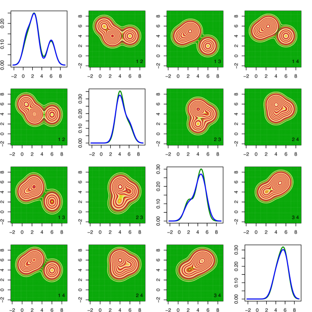
Figure 4: Results for the $f_{{\mathbf{X}}}$ produced by the MLFA (mixtures of latent factor analyzers) method for the conditionally heteroscedastic error distribution $f_{\mbox{\boldmath$\epsilon$}}^{(2)}$ with sample size $n=1000$, $m_{i}=3$ replicates for each subject and identity matrix (I) for the component specific covariance matrices. The results correspond to the data set that produced the median of the estimated integrated squared errors (ISE) out of a total of 100 simulated data sets. See Section 6 for additional details. The upper triangular panels show the contour plots of the true two dimensional marginal densities. The lower triangular diagonally opposite panels show the corresponding estimates. The numbers $i,j$ at the bottom right corners of the off-diagonal panels show that the marginal densities $f_{X_{i},X_{j}}$ are plotted in those panels. The diagonal panels show the true (lighter shaded green lines) and the estimated (darker shaded blue lines) one dimensional marginals. The figure is in color in the electronic version of this article.

The parameters were chosen to produce a wide variety of one and two dimensional marginal densities, see Figure 4 and also Figure 6. Scale adjustments by multiplication with ${\mathbf{D}}_{{\mathbf{X}}}$ and ${\mathbf{D}}_{\mbox{\boldmath$\epsilon$}}$ were done so that the simulated values of each component of ${\mathbf{X}}$ fall essentially in the range $(-2,6)$ and the simulated values of all components of $\epsilon$ fall essentially in the range $(-3,3)$. For conditionally heteroscedastic measurement errors, we set the true variance functions at $s_{\ell}^{2}(X)=(1+X/4)^{2}$ for each component $\ell$. A total of $16~{}(2\times 1\times 2\times 4)$ cases were thus considered for both independent and conditionally heteroscedastic measurement errors.

We first discuss the results of the simulation experiments when the measurement errors ${\mathbf{U}}$ were independent of ${\mathbf{X}}$. The estimated MISEs are presented in Table 1. When the true $f_{\mbox{\boldmath$\epsilon$}}$ was a single component multivariate normal, the MLFA model produced the lowest MISE when the true covariance matrices were diagonal. In all other cases the MIW model produced the best results. When the true $f_{\mbox{\boldmath$\epsilon$}}$ was a mixture of multivariate normals, the model complexity increases and the performance of the MIW model started to deteriorate. In this case, the MLFA model dominated the MIW model when the true covariance matrices were either diagonal or had a latent factor characterization.

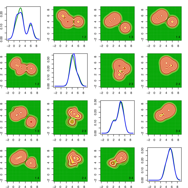
Figure 3: Results for $f_{{\mathbf{X}}}$ produced by the MIW (mixtures with inverse Wishart priors) method for the conditionally heteroscedastic error distribution $f_{\mbox{\boldmath$\epsilon$}}^{(2)}$ with sample size $n=1000$, $m_{i}=3$ replicates for each subject and identity matrix (I) for the component specific covariance matrices. The results correspond to the data set that produced the median of the estimated integrated squared errors (ISE) out of a total of 100 simulated data sets. See Section 6 for additional details. The upper triangular panels show the contour plots of the true two dimensional marginal densities. The lower triangular diagonally opposite panels show the corresponding estimates. The numbers $i,j$ at the bottom right corners of the off-diagonal panels show that the marginal densities $f_{X_{i},X_{j}}$ are plotted in those panels. The diagonal panels show the true (lighter shaded green lines) and the estimated (darker shaded blue lines) one dimensional marginals. The figure is in color in the electronic version of this article.

The estimated MISEs for the cases when ${\mathbf{U}}$ were conditionally heteroscedastic are presented in Table 2. Models that accommodate conditional heteroscedasticity are significantly more complex compared to models that assume independence of the measurement errors from ${\mathbf{X}}$. The numerically more stable MLFA model thus out-performed the MIW model in all 32 cases. The improvements were particularly significant when the true covariance matrices were sparse and the number of subjects was small ($n=500$). The true and estimated univariate and bivariate marginals of $f_{{\mathbf{X}}}$ produced by the MIW and the MLFA methods when the true density of the scaled errors was a mixture of multivariate normals ($f_{\mbox{\boldmath$\epsilon$}}^{(2)}$) and the component specific covariance matrices were diagonal (I) are summarized in Figure 3 and Figure 4, respectively. The true and estimated univariate and bivariate marginals for the density of the scaled errors $f_{\mbox{\boldmath$\epsilon$}}$ for this case produced by the two methods are summarized in Figure 5 and Figure 6, respectively. The true and the estimated variance functions produced by the univariate submodels are summarized in Figure 2. Comparisons between Figure 3 and Figure 4 illustrate the limitations of the MIW models in capturing high dimensional sparse covariance matrices and the improvements that can be achieved by the MLFA models. The estimates of $f_{\mbox{\boldmath$\epsilon$}}$ produced by the two methods are in better agreement. This may be attributed to the fact that many more residuals are available for estimating $f_{\mbox{\boldmath$\epsilon$}}$ than there are ${\mathbf{X}}_{i}$’s to estimate $f_{{\mathbf{X}}}$. Figure 2 in the main paper and Figures S.7 and S.16 in the Supplementary Materials show that the univariate submodels can recover the true variance functions well. Additional figures when the true covariance matrices had auto-regressive structure (AR) are presented in the Supplementary Materials. In this case the true covariance matrices were not sparse. The MLFA method still vastly dominated the MIW method when the sample size was small ($n=500$). When the sample size was large ($n=1000$) the two methods produced comparable results.

The proposed deconvolution methods, in particular the MLFA method, are highly scalable. In small scale simulations, not reported here, we tried $p=6,8$ and $10$ and observed good empirical performance. We have focused here on $p=4$ dimensional problems since with $p=4$ the numbers of univariate and bivariate marginals, $p=4$ and ${p\choose 2}=6$, remain manageable and the results are conveniently graphically summarized.

Additional small scale simulations for a variety of other distributions with similar MISE patterns are presented in the Supplementary Materials.

7 Example

Dietary habits are known to be leading causes of many chronic diseases. Accurate estimation of the distributions of dietary intakes is thus important in nutritional epidemiologic surveillance and epidemiology. Nutritionists are typically interested not just in the consumption patterns of individual dietary components but also in their joint consumption patterns. By the very nature of the problem, ${\mathbf{X}}$, the average long term daily intakes of the dietary components, can never be directly observed. Data are thus typically collected from a representative sample of the population in the form of dietary recalls, the subjects participating in the study remembering and reporting the type and amount of food they had consumed in the past 24 hours. The problem of estimating the joint consumption pattern of the dietary components from the contaminated 24-hour recalls then becomes a problem of multivariate density deconvolution.

A large scale epidemiologic study conducted by the National Cancer Institute, the Eating at America’s Table (EATS) study (Subar, et al. 2001), serves as the motivation for this paper. In this study $n=965$ participants were interviewed $m_{i}=4$ times over the course of a year and their 24 hour dietary recalls (${\mathbf{W}}_{ij}$’s) were recorded. The goal is to estimate the joint consumption patterns of the true daily intakes (${\mathbf{X}}_{i}$’s).

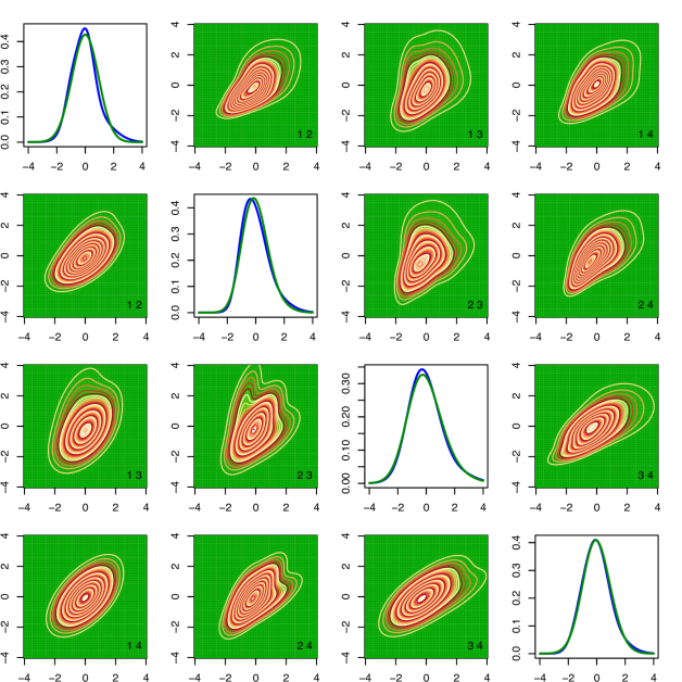
Figure 9: Results for the EATS data set for the density of the scaled errors $f_{\mbox{\boldmath$\epsilon$}}$. The off-diagonal panels show the contour plots of two-dimensional marginals estimated by the MIW method (upper triangular panels) and the MLFA method (lower triangular panels). The numbers $i,j$ at the bottom right corners of the off-diagonal panels show that the marginal densities $f_{\epsilon_{i},\epsilon_{j}}$ are plotted in those panels. The diagonal panels show the one dimensional marginal densities estimated by the MIW method (darker shaded blue lines) and the MLFA method (lighter shaded green lines). The figure is in color in the electronic version of this article.

To illustrate our methodology, we consider the problem of estimating the joint consumption pattern of four dietary components, namely (a) carbohydrate, (b) fiber, (c) protein and (d) a mineral potassium. Figure 7 shows the plots of subject-specific means versus subject-specific variances for daily intakes of the dietary components with the estimates of the variance functions produced by univariate submodels superimposed over them. As is clearly identifiable from this plot, conditional heteroscedasticity is a very prominent feature of the measurements errors contaminating the 24 hour recalls. The estimated univariate and bivariate marginal densities of average long term daily intakes of the dietary components produced by the MIW method and the MLFA method are summarized in Figure 8. The estimated univariate and bivariate marginal densities for the scaled errors are summarized in Figure 9. The estimated marginals of ${\mathbf{X}}$ produced by the two methods look quite different, while the estimated marginals of $\epsilon$ are in close agreement. The estimated univariate and bivariate marginal densities of the long term intakes of the dietary components produced by the MIW model look irregular and unstable, whereas the estimates produced by the MLFA model look relatively more regular and stable. In experiments not reported here, we observed that the estimates produced by the MIW method were sensitive to the choice of the number of mixture components, but the estimates produced by the MLFA model were quite robust. The trace plots and the frequency distributions of the of the numbers of nonempty mixture components are summarized in Figures S.14 and S.15 in the Supplementary Materials and provide some idea about the relative stability of the two methods. These observations are similar to that made in Section 6 for conditionally heteroscedastic measurement errors and sparse covariance matrices.

We next comment only on the estimates produced by the MLFA method assuming them to be closer to the truth. The estimates show that the long term daily intakes of the four dietary components are strongly correlated. The shapes of the bivariate consumption patterns suggest deviations from normality. Similarly, the shapes of the bivariate marginals for the scaled errors suggest that the measurement errors in the reported 24 hour recalls are positively correlated and deviate from normality. People who consume more are expected to do so for most dietary components. Strong correlations between the intakes of the dietary components are thus somewhat expected. The correlations among different components of the measurement errors suggest that people usually have a tendency to either over-report or under-report the daily intakes. These findings illustrate the importance of robust but numerically stable multivariate deconvolution methods in nutritional epidemiologic studies.

Additional discussions on potentially far-reaching impact of our work on nutritional epidemiology studies are deferred to Section S.10 in the Supplementary Materials.

8 Discussion

We considered the problem of multivariate density deconvolution when the measurement error density is not known but replicated proxies are available for some individuals. We used flexible finite mixtures of multivariate normal kernels with symmetric Dirichlet priors on the mixture probabilities to model both the density of interest and the density of the measurement errors. We proposed a novel technique to make the model for the density of the errors satisfy a zero mean restriction. We showed that the dense parametrization of inverse Wishart priors are not suitable for modeling covariance matrices in the presence of measurement errors. We proposed a numerically more stable approach based on latent factor characterization of the covariance matrices with sparsity inducing priors on the factor loading matrices. We built models for conditionally heteroscedastic additive measurement errors that also automatically accommodate multivariate multiplicative measurement errors.

The methodological contributions of this article are not limited to deconvolution problems. Mixtures of latent factor analyzers with sparsity inducing priors on the factor loading matrices can be used in other high dimensional applications including ordinary density estimation. The techniques proposed in Section 2.2.1 to enforce the mean zero moment restriction on the measurement errors can be readily used to model multivariate regression errors that are distributed independently of the predictors. The technique can also be adapted to relax the strong assumption of multivariate normality made by Hoff and Niu (2012) and Fox and Dunson (2016) in covariance regression problems.

As explained in Sections 2.2.2 and 2.2.3 in the main paper and also in Section S.5 in the Supplementary Materials, the structural separability assumption (24) arises naturally in both additive and multiplicative multivariate measurement error settings. It would still be interesting, in future work, to consider more general covariance models that allow $\hbox{var}(U_{ij\ell}|{\mathbf{X}})$ to be explained primarily by $X_{i\ell}$, as in the current approach, but would allow the residual variability to be explained by the remaining components $\{X_{im}\}_{m\neq\ell}$ of ${\mathbf{X}}$. The current MCMC based implementation of the proposed methodology is computationally intensive. We are pursuing the development of faster algorithms for approximate posterior inference as the subject of a separate manuscript.

The question of consistency of Bayesian procedures is intimately related to the flexibility of the priors. For instance, in ordinary density estimation problems inclusion of the true density in the KL support of the prior is a sufficient condition to ensure weak consistency via the Schwartz theorem. In density deconvolution problems such a condition is not sufficient but is still required. The results from Section 5 thus provide crucial first steps in that direction. We have not pursued the question of consistency of the proposed deconvolution methods any further in this article. It remains an important direction for future research.

Supplementary Materials

The Supplementary Materials discuss the choice of hyper-parameters and MCMC algorithms to sample from the posterior, including the two-stage estimation procedure for conditionally heteroscedastic measurement errors. The Supplementary Materials also present our arguments in favor of finite mixture models, pointing out how their close connections and their subtle differences with possible infinite dimensional alternatives are exploited to achieve significant reduction in computational complexity while retaining the major advantages of infinite dimensional mixture models including model flexibility and automated model selection and model averaging. The Supplementary Materials additionally present discussions on the contrasts between regression and measurement errors that preclude the use of covariance regression techniques to model conditionally heteroscedastic measurement errors, the proofs of the theoretical results presented in Section 5, some additional figures, and results of additional simulation experiments. R programs implementing the deconvolution methods for conditionally heteroscedastic errors are included as part of the Supplementary Materials. The EATS data analyzed in Section 7 can be accessed from National Cancer Institute by arranging a Material Transfer Agreement. A simulated data set, simulated according to one of the designs described in Section 6, and a ‘readme’ file providing additional details are also included in the Supplementary Materials.

References

Bhattacharya, A. and Dunson, D. B. (2011). Sparse Bayesian infinite factor models. Biometrika, 98, 291-306.

Bhattacharya, A., Pati, D., Pillai, N. and Dunson, D. B. (2014). Bayesian shrinkage. Unpublished manuscript.

Brown, P. J. and Griffin, J. E. (2010). Inference with normal-gamma prior distributions in regression problems. Bayesian Analysis, 5, 171-188.

Bovy, J., Hogg, D. W. and Rowies, S. T. (2011). Extreme deconvolution: inferring complete distribution functions from noisy, heterogeneous and incomplete observations. Annals of Applied Statistics, 5, 1657-1677.

Buonaccorsi, J. P. (2010). Measurement Error: Models, Methods and Applications. New York: Chapman and Hall/CRC.

Carroll, R. J. and Hall, P. (1988). Optimal rates of convergence for deconvolving a density. Journal of the American Statistical Association, 83, 1184-1186.

Carroll, R. J. and Hall, P. (2004). Low order approximations in deconvolution and regression with errors in variables. Journal of the Royal Statistical Society, Series B, 66, 31-46.

Carroll, R. J., Ruppert, D., Stefanski, L. A. and Crainiceanu, C. M. (2006). Measurement Error in Nonlinear Models (2nd ed.). Boca Raton: Chapman and Hall/CRC Press.

Carvalho, M. C., Polson, N. G. and Scott, J. G. (2010). The horseshoe estimator for sparse signals. Biometrika, 97, 465-480.

Comte, F. and Lacour, C. (2013). Anisotropic adaptive density deconvolution. Annales de l’Institut Henri Poincaré - Probabilités et Statistiques, 49, 569-609.

Devroye, L. (1989). Consistent deconvolution in density estimation. Canadian Journal of Statistics, 17, 235-239.

Diggle, P. J. and Hall, P. (1993). A Fourier approach to nonparametric deconvolution of a density estimate. Journal of the Royal Statistical Society, Series B, 55, 523-531.

Eilers, P. H. C. and Marx, B. D. (1996). Flexible smoothing with B-splines and penalties. Statistical Science, 11, 89-121.

Fan, J. (1991a). On the optimal rates of convergence for nonparametric deconvolution problems. Annals of Statistics, 19, 1257-1272.

Fan, J. (1991b). Global behavior of deconvolution kernel estimators. Statistica Sinica, 1, 541-551.

Fan, J. (1992). Deconvolution with supersmooth distributions. Canadian Journal of Statistics, 20, 155-169.

Fokoué, E. and Titterington, D. M. (2003). Mixtures of factor analyzers. Bayesian estimation and inference by stochastic simulation. Machine Learning, 50, 73-94.

Fox, E. B. and Dunson, D. (2016). Bayesian nonparametric covariance regression. To appear in Journal of Machine Learning Research.

Frühwirth-Schnatter, S. (2006). Finite Mixture and Markov Switching Models. New York: Springer.

Geweke, J. (2007). Interpretation and inference in mixture models: Simple MCMC works. Computational Statistics & Data Analysis, 51, 3529-3550.

Hazelton, M.L. and Turlach, B.A. (2009). Nonparametric density deconvolution by weighted kernel estimators. Statistics and Computing, 19, 217-228.

Hazelton, M.L. and Turlach, B.A. (2010). Semiparametric density deconvolution. Scandinavian Journal of Statistics, 37, 91-108.

Hesse, C. H. (1999). Data driven deconvolution. Journal of Nonparametric Statistics, 10, 343-373.

Hoff, P. D. and Niu, X. (2012). A covariance regression model. Statistica Sinica, 22, 729-753.

Hu, Y and Schennach, S. (2008). Instrumental Variable Treatment of Nonclassical Measurement Error Models. Econometrica, 76, 195-216.

Li, T. and Vuong, Q. (1998). Nonparametric estimation of the measurement error model using multiple indicators. Journal of Multivariate Analysis, 65, 139-165.

Liu, M. C. and Taylor, R. L. (1989). A consistent nonparametric density estimator for the deconvolution problem. Canadian Journal of Statistics, 17, 427-438.

Masry, E. (1991). Multivariate probability density deconvolution for stationary random processes. IEEE Transactions on Information Theory, 37, 1105-1115.

Mengersen, K. L., Robert, C. P. and Titterington, D. M. (eds) (2011). Mixtures - Estimation and Applications. Chichester: John Wiley.

Neumann, M. H. (1997). On the effect of estimating the error density in nonparametric deconvolution. Journal of Nonparametric Statistics, 7, 307-330.

Sarkar, A., Mallick, B. K., Staudenmayer, J., Pati, D. and Carroll, R. J. (2014). Bayesian semiparametric density deconvolution in the presence of conditionally heteroscedastic measurement errors. Journal of Computational and Graphical Statistics, 23, 1101-1125.

Schennach, S. (2004). Nonparametric regression in the presence of measurement error. Econometric Theory, 20, 1046-1093.

Staudenmayer, J., Ruppert, D. and Buonaccorsi, J. P. (2008). Density estimation in the presence of heteroscedastic measurement error. Journal of the American Statistical Association, 103, 726-736.

Subar, A. F., Thompson, F. E., Kipnis, V., Midthune, D., Hurwitz, P. McNutt, S., McIntosh, A. and Rosenfeld, S. (2001). Comparative validation of the block, Willet, and National Cancer Institute food frequency questionnaires. American Journal of Epidemiology, 154, 1089-1099.

Youndjé, E. and Wells, M. T. (2008). Optimal bandwidth selection for multivariate kernel deconvolution. TEST, 17, 138-162.

True Error Distribution	Covariance Structure	Sample Size	MISE $\times 10^{4}$
			MLFA	MIW	Naive
(a) Multivariate Normal	I	500	1.24	3.05	8.01
		1000	0.59	1.33	6.58
	LF	500	6.88	6.33	33.41
		1000	5.15	3.10	32.42
	AR	500	11.91	5.51	27.17
		1000	9.82	2.78	26.01
	EXP	500	7.15	4.40	17.82
		1000	5.46	2.19	17.40
(b) Mixture of Multivariate Normal	I	500	1.28	3.24	5.97
		1000	0.64	1.37	4.99
	LF	500	7.28	7.51	31.62
		1000	4.17	4.34	31.48
	AR	500	10.43	6.66	30.74
		1000	7.75	4.35	28.90
	EXP	500	7.16	5.18	17.85
		1000	4.87	2.66	17.26

Table 1: Mean integrated squared error (MISE) performance of MLFA (mixtures of latent factor analyzers) and MIW (mixtures with inverse Wishart priors) density deconvolution models described in Section 2 of this article for homoscedastic errors compared with a naive method that ignores measurement errors for different measurement error distributions. The minimum value in each row is highlighted.

True Error Distribution	Covariance Structure	Sample Size	MISE $\times 10^{4}$
			MLFA	MIW	Naive
(a) Multivariate Normal	I	500	2.53	19.08	10.64
		1000	1.15	9.43	9.14
	LF	500	11.46	34.21	21.33
		1000	5.78	15.98	20.75
	AR	500	17.11	30.83	36.44
		1000	10.77	12.46	36.37
	EXP	500	11.63	26.99	24.28
		1000	6.67	10.56	23.36
(b) Mixture of Multivariate Normal	I	500	2.79	22.17	20.16
		1000	1.38	10.55	19.39
	LF	500	13.39	35.67	43.43
		1000	7.50	20.86	43.28
	AR	500	18.27	35.70	75.26
		1000	12.06	16.64	77.55
	EXP	500	12.11	34.50	48.76
		1000	7.59	13.74	50.02

Table 2: Mean integrated squared error (MISE) performance of MLFA (mixtures of latent factor analyzers) and MIW (mixtures with inverse Wishart priors) density deconvolution models described in Section 2 of this article for conditionally heteroscedastic errors compared with a naive method that ignores measurement errors for different measurement error distributions. The minimum value in each row is highlighted.

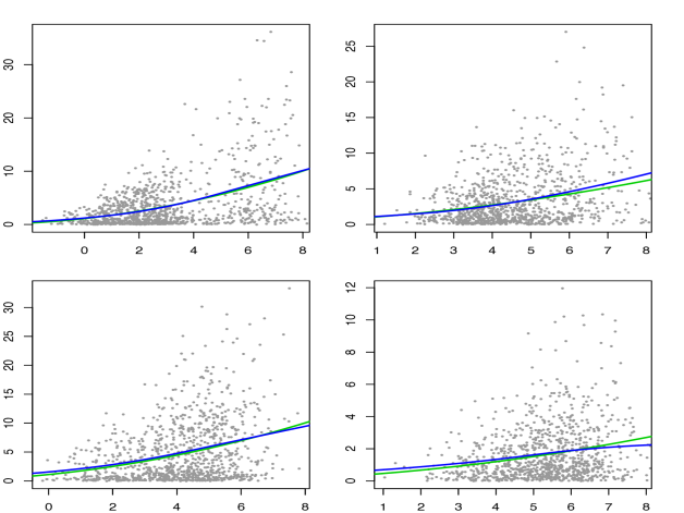
Figure 2: Results for conditional variability $\hbox{var}(U|X)=s^{2}(X)\hbox{var}(\epsilon)$ produced by the univariate density deconvolution method for each component of ${\mathbf{X}}$ for the conditionally heteroscedastic error distribution $f_{\mbox{\boldmath$\epsilon$}}^{(2)}$ with sample size $n=1000$, $m_{i}=3$ replicates for each subject and identity matrix (I) for the component specific covariance matrices. The results correspond to the data set that produced the median of the estimated integrated squared errors (ISE) out of a total of 100 simulated data sets for the MLFA (mixtures of latent factor analyzers) method. For each component of ${\mathbf{X}}$, the true variance function is $s^{2}(X)=(1+X/4)^{2}$. See Section 2.2.2 and Section S.3 for additional details. In each panel, the true (lighter shaded green lines) and the estimated (darker shaded blue lines) variance functions are superimposed over a plot of subject specific sample means vs subject specific sample variances. The figure is in color in the electronic version of this article.

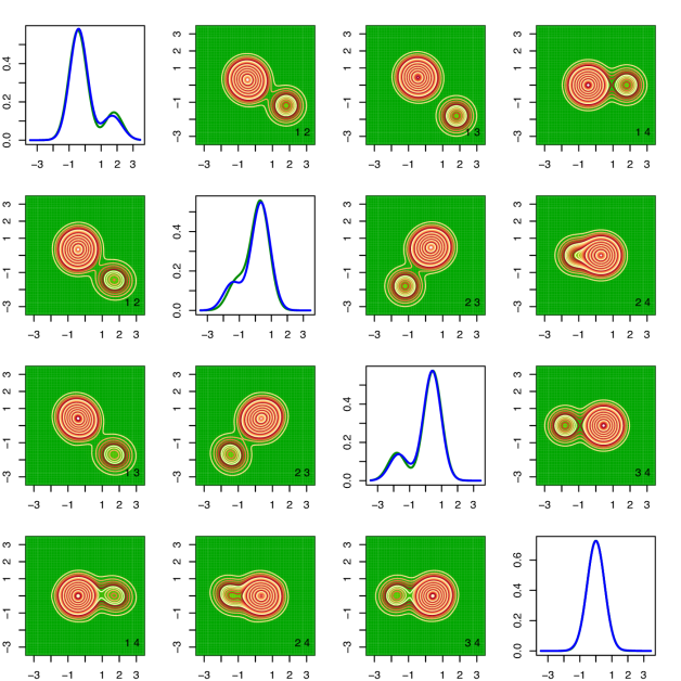
Figure 5: Results for the density of the scaled measurement errors $f_{\mbox{\boldmath$\epsilon$}}$ produced by the MIW (mixtures with inverse Wishart priors) method for the conditionally heteroscedastic error distribution $f_{\mbox{\boldmath$\epsilon$}}^{(2)}$ with sample size $n=1000$, $m_{i}=3$ replicates for each subject and identity matrix (I) for the component specific covariance matrices. The results correspond to the data set that produced the median of the estimated integrated squared errors (ISE) out of a total of 100 simulated data sets. See Section 6 for additional details. The upper triangular panels show the contour plots of the true two dimensional marginal densities. The lower triangular diagonally opposite panels show the corresponding estimates. The numbers $i,j$ at the bottom right corners of the off-diagonal panels show that the marginal densities $f_{\epsilon_{i},\epsilon_{j}}$ are plotted in those panels. The diagonal panels show the true (lighter shaded green lines) and the estimated (darker shaded blue lines) one dimensional marginals. The figure is in color in the electronic version of this article.

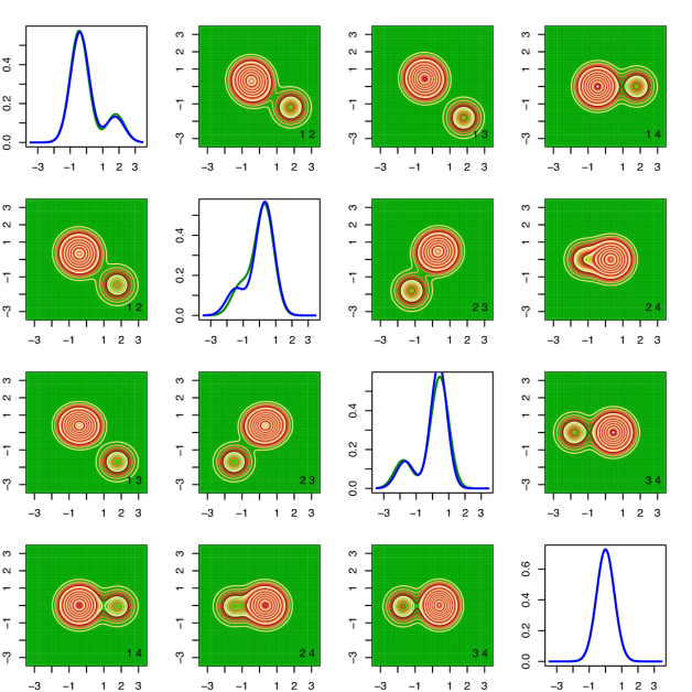
Figure 6: Results for the density of the scaled measurement errors $f_{\mbox{\boldmath$\epsilon$}}$ produced by the MLFA (mixtures of latent factor analyzers) method for the conditionally heteroscedastic error distribution $f_{\mbox{\boldmath$\epsilon$}}^{(2)}$ with sample size $n=1000$, $m_{i}=3$ replicates for each subject and identity matrix (I) for the component specific covariance matrices. The results correspond to the data set that produced the median of the estimated integrated squared errors (ISE) out of a total of 100 simulated data sets. See Section 6 for additional details. The upper triangular panels show the contour plots of the true two dimensional marginal densities. The lower triangular diagonally opposite panels show the corresponding estimates. The numbers $i,j$ at the bottom right corners of the off-diagonal panels show that the marginal densities $f_{\epsilon_{i},\epsilon_{j}}$ are plotted in those panels. The diagonal panels show the true (lighter shaded green lines) and the estimated (darker shaded blue lines) one dimensional marginals. The figure is in color in the electronic version of this article.

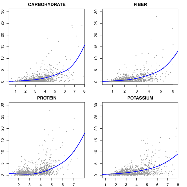
Figure 7: Estimated variance functions $\hbox{var}(U|X)=s^{2}(X)\hbox{var}(\epsilon)$ produced by the univariate density deconvolution method for each component of ${\mathbf{X}}$ for the EATS data set with sample size $n=965$, $m_{i}=4$ replicates for each subject. See Section 7 for additional details. The figure is in color in the electronic version of this article.

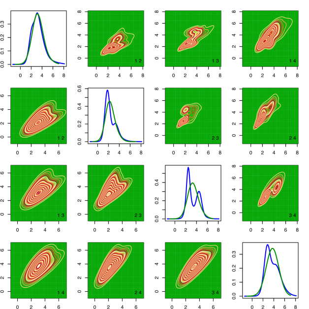
Figure 8: Results for the EATS data set for the $f_{{\mathbf{X}}}$. The off-diagonal panels show the contour plots of two-dimensional marginals estimated by the MIW method (upper triangular panels) and the MLFA method (lower triangular panels). The numbers $i,j$ at the bottom right corners of the off-diagonal panels show that the marginal densities $f_{X_{i},X_{j}}$ are plotted in those panels. The diagonal panels show the one dimensional marginal densities estimated by the MIW method (darker shaded blue lines) and the MLFA method (lighter shaded green lines). The figure is in color in the electronic version of this article.

Supplementary Materials for
Bayesian Semiparametric Multivariate Density Deconvolution

Abhra Sarkar

Department of Statistical Science, Duke University, Durham, NC 27708-0251, USA

abhra.sarkar@duke.edu

Debdeep Pati

Department of Statistics, Florida State University, Tallahassee, FL 32306-4330, USA

debdeep@stat.fsu.edu

Bani K. Mallick

Department of Statistics, Texas A&M University, 3143 TAMU, College Station,

TX 77843-3143, USA

bmallick@stat.tamu.edu

Raymond J. Carroll

Department of Statistics, Texas A&M University, 3143 TAMU, College Station,

TX 77843-3143, USA

and School of Mathematical and Physical Sciences, University of Technology Sydney, Broadway NSW 2007, Australia

carroll@stat.tamu.edu

The Supplementary Materials are organized as follows. Section S.1 discusses the choice of hyper-parameters. In Section S.2, we describe a Gibbs sampler for drawing samples from the posterior of the deconvolution model for multivariate independently distributed homoscedastic errors, described in Section 2.2.1 of the main paper. In Section S.3, we detail a two stage estimation procedure for drawing samples from the posterior of the deconvolution model for multivariate conditionally heteroscedastic measurement errors described in Section 2.2.2 of the main paper. Section S.4 provides heuristic justification for the two-stage sampler. In Section S.5, we provide additional detailed discussion of the model for multivariate conditionally heteroscedastic measurement errors described in Section 2.2.2 of the main paper, contrasting it with models for multivariate conditionally varying regression errors (Section S.5.1), its connections with latent factor models (Section S.5.2), its flexibility, limitations, and plausible generalizations (Section S.5.3), and tools for model adequacy checks (Section S.5.4). Section S.6 presents our arguments in favor of finite mixture models, pointing out how their close connections and their subtle differences with possible infinite dimensional alternatives are exploited to achieve significant reduction in computational complexity (Section S.6.2) while retaining the major advantages of infinite dimensional mixture models including model flexibility (Section S.6.4) and automated model selection and model averaging (Section S.6.3). Section S.7 details proofs of the theoretical results presented in Section 5 of the main paper. Section S.8 presents additional figures related to the simulation experiments discussed in Section 6 of the main paper. Section S.9 presents results of additional simulation experiments. Section S.10 discusses potentially far-reaching impact of our work in nutritional epidemiology.

S.1 Choice of Hyper-Parameters

We discuss the choice of hyper-parameters in this section. To avoid unnecessary repetition, in this section and onwards, symbols sans the subscripts ${\mathbf{X}}$ and $\epsilon$ are sometimes used as generics for similar components and parameters of the models. For example, $K$ is a generic for $K_{{\mathbf{X}}}$ and $K_{\mbox{\boldmath$\epsilon$}}$; $\mbox{\boldmath$\mu$}_{k}$ is a generic for $\mbox{\boldmath$\mu$}_{{\mathbf{X}},k}$ and $\mbox{\boldmath$\mu$}_{\mbox{\boldmath$\epsilon$},k}$; and so on.

1. Number of mixture components: Practical application of our method requires that a decision be made on the number of mixture components $K_{{\mathbf{X}}}$ and $K_{\mbox{\boldmath$\epsilon$}}$ in the models for the densities $f_{{\mathbf{X}}}$ and $f_{\mbox{\boldmath$\epsilon$}}$, respectively.

   Our simulation experiments suggest that when the true densities are finite mixtures of multivariate normals and $K_{{\mathbf{X}}}$ and $K_{\mbox{\boldmath$\epsilon$}}$ are assigned values greater than the corresponding true numbers, the MCMC chain often quickly reaches a steady state where the redundant components become empty. See Figures S.6, S.12 and S.13 in the Supplementary Materials for illustrations. These observations are similar to that made in the context of ordinary density estimation by Rousseau and Mengersen (2011) who studied the asymptotic behavior of the posterior for overfitted mixture models and showed that when $\alpha/K<L/2$, where $L$ denotes the number of parameters specifying the component kernels, the posterior is stable and concentrates in regions with empty redundant components. We set $\alpha_{{\mathbf{X}}}=\alpha_{\mbox{\boldmath$\epsilon$}}=1$ so that the condition $\alpha/K<L/2$ is satisfied.

   Educated guesses about $K_{{\mathbf{X}}}$ and $K_{\mbox{\boldmath$\epsilon$}}$ may nevertheless be useful in safeguarding against gross overfitting that would result in a wastage of computation time and resources. The following simple strategies may be employed. Model based cluster analysis techniques as implemented by the mclust package in R (Fraley and Raftery, 2007) may be applied to the starting values of ${\mathbf{X}}_{i}$ and the corresponding residuals, obtained by fitting univariate submodels for each component of ${\mathbf{X}}$, to get some idea about $K_{{\mathbf{X}}}$ and $K_{\mbox{\boldmath$\epsilon$}}$. The chain may be started with larger values of $K_{{\mathbf{X}}}$ and $K_{\mbox{\boldmath$\epsilon$}}$ and after a few hundred iterations the redundant empty components may be deleted on the fly.

   As shown in Section 5, our methods can approximate a large class of data generating densities, and we found the strategy described above to be very effective in all cases we experimented with. The parameter $\alpha$ now plays the role of a smoothing parameter, smaller values favoring a smaller number of mixture components and thus smoother densities. In simulation experiments involving multivariate t and multivariate Laplace distributions reported in the Supplementary Materials, and in some other cases not reported here, the values $\alpha_{{\mathbf{X}}}=\alpha_{\mbox{\boldmath$\epsilon$}}=1$ worked well.

   As we discuss in Section 6, the MIW method becomes highly numerically unstable when the measurement errors are conditionally heteroscedastic and the true covariance matrices are highly sparse. In these cases in particular, the MIW method usually requires much larger sample sizes for the asymptotic results to hold and in finite samples the above mentioned strategy usually overestimates the required number of mixture components. See Figure S.5 in the Supplementary Materials for an illustration. Since mixtures based on $(K+1)$ components are at least as flexible as mixtures based on $K$ components, as far as model flexibility is concerned, such overestimation is not an issue. But since this also results in clusters of smaller sizes, the estimates of the component specific covariance matrices become numerically even more unstable, further compounding the stability issues of the MIW model. In contrast, for the numerically more stable MLFA model, for the exact opposite reasons, the asymptotic results are valid for moderate sample sizes and such models are also more robust to overestimation of the number of nonempty clusters.

2. Number of latent factors: For the MLFA method, the MCMC algorithm summarized in Section S.2 also requires that the component specific infinite factor models be truncated at some appropriate truncation level. The shrinkage prior again makes the model highly robust to overfitting allowing us to adopt a simple strategy. Since a latent factor characterization leads to a reduction in the number or parameters only when $q_{k}\leq\lceil(p+1)/2\rceil$, where $\lceil s\rceil$ denotes the largest integer smaller than or equals to $s$, we simply set the truncation level at $q_{k}=q=\max\{2,\lceil(p+1)/2\rceil\}$ for all the components. We also experimented by setting the truncation level at $q_{k}=q=p$ for all $k$ with the results remaining practically the same. The shrinkage prior, being continuous in nature, does not set the redundant columns to exact zeroes, but it adaptively shrinks the redundant parameters sufficiently towards zero, thus producing stable and efficient estimates of the densities being modeled.

3. Other hyper-parameters: We take an empirical Bayes type approach to assign values to other hyper-parameters. We set $\mbox{\boldmath$\mu$}_{{\mathbf{X}},0}=\overline{{\mathbf{X}}}^{(0)}$, the overall mean of ${{\mathbf{X}}}_{1:n}^{(0)}$, where ${\mathbf{X}}_{1:n}^{(0)}$ denote the starting values of ${\mathbf{X}}_{1:n}$ for the MCMC sampler discussed in Section S.2. For the scaled errors we set $\mbox{\boldmath$\mu$}_{\mbox{\boldmath$\epsilon$},0}={\mathbf{0}}$. For the MIW model we take $\nu_{0}=(p+2)$, the smallest possible integral value of $\nu_{0}$ for which the prior mean of $\mbox{\boldmath$\Sigma$}_{k}$ exists. We then take $\mbox{\boldmath$\Sigma$}_{{\mathbf{X}},0}/2=\mbox{\boldmath$\Psi$}_{{\mathbf{X}},0}=\hbox{cov}(\overline{{\mathbf{X}}}_{1:n}^{(0)})$. These choices imply $E(\mbox{\boldmath$\Sigma$}_{{\mathbf{X}},k})=\mbox{\boldmath$\Psi$}_{{\mathbf{X}},0}=\hbox{cov}(\overline{{\mathbf{X}}}^{(0)})$ and, since the variability of each component is expected to be significantly less than the overall variability, ensure noninformativeness. Similarly, for the scaled errors we take $\mbox{\boldmath$\Sigma$}_{\mbox{\boldmath$\epsilon$},0}/2=\mbox{\boldmath$\Psi$}_{\mbox{\boldmath$\epsilon$},0}=\hbox{cov}(\mbox{\boldmath$\epsilon$}_{1:N}^{(0)})$. For the MLFA model, the hyper-parameters specifying the prior for $\Lambda$ are set at $a_{1}=1,a_{h}=2$ for all $h\geq 2$, and $\nu=1$. Inverse gamma priors with parameters $a_{\sigma}=1.1,b_{\sigma}=1$ are placed on the elements of $\Omega$. For each $k$, the variance functions were modeled using quadratic (q=2) B-splines based on $(2\times 2+5+1)=10$ equidistant knot points on $[A_{k},B_{k}]=[\hbox{min}(\overline{{\mathbf{W}}}_{k,1:n})-0.1~{}\hbox{range}(\overline{{\mathbf{W}}}_{k,1:n}),\hbox{max}(\overline{{\mathbf{W}}}_{k,1:n})+0.1~{}\hbox{range}(\overline{{\mathbf{W}}}_{k,1:n})]$, where $\overline{{\mathbf{W}}}_{\ell,1:n}$ denotes the subject specific means corresponding to $\ell^{th}$ component.

S.2 Posterior Computation

Samples from the posterior can be drawn using Gibbs sampling techniques. In what follows $\zeta$ denotes a generic variable that collects the observed proxies ${\mathbf{W}}_{1:N}$ and all the parameters of a model, including the imputed values of ${\mathbf{X}}_{1:n}$ and $\mbox{\boldmath$\epsilon$}_{1:N}$, that are not explicitly mentioned.

Carefully chosen starting values can facilitate convergence of the sampler. The posterior means of the $X_{i\ell}$’s, obtained by fitting univariate submodels, are used as the starting values for the multivariate sampler. The number of mixture components are initialized at $K_{{\mathbf{X}}}=(m_{{\mathbf{X}}}+2)$, where $m_{{\mathbf{X}}}$ denotes the optimal number of clusters returned by model based clustering algorithm implemented by the mclust package in R applied to the corresponding initial values ${\mathbf{X}}_{1:n}^{(0)}$. The component specific mean vectors of the nonempty clusters are set at the mean of ${\mathbf{X}}_{i}^{(0)}$ values that belong to that cluster. The component specific mean vectors of the two empty clusters are set at $\overline{{\mathbf{X}}}^{(0)}$, the overall mean of ${{\mathbf{X}}}_{1:n}^{(0)}$. For the MIW model, the initial values of the cluster specific covariance matrices are chosen in a similar fashion. The mixture probabilities for the $k^{th}$ nonempty cluster is set at $\mbox{\boldmath$\pi$}_{{\mathbf{X}},k}=n_{k}/n$, where $n_{k}$ denotes the number of ${\mathbf{X}}_{i}^{(0)}$ belonging to the $k^{th}$ cluster. The mixture probabilities of the empty clusters are initialized at zero. For the MLFA method, the starting values of all elements of $\Lambda$ and $\eta$ are set at zero. The starting values for the elements of $\Omega$ are chosen to equal the variances of the corresponding starting values. The parameters specifying the density of the scaled errors are initialized in a similar manner. The MCMC iterations comprise the following steps. We suppress the subscript $\epsilon$ to keep the notation clean as in the main paper.

1. Updating the parameters specifying $f_{{\mathbf{X}}}$: For the MIW model the parameters specifying the density $f_{{\mathbf{X}}}$ are updated using the following steps.
   

   $$(\mbox{\boldmath$\pi$}|\mbox{\boldmath$\zeta$}) \sim \hbox{Dir}(\alpha/K+n_{1},\alpha/K+n_{2},\dots,\alpha/K+n_{K}),$$

   $$(C_{i}|\mbox{\boldmath$\zeta$}) \sim \hbox{Mult}(1,p_{i1},p_{i2},\dots,p_{iK}),$$

   $$(\mbox{\boldmath$\mu$}_{k}|\mbox{\boldmath$\zeta$}) \sim \hbox{MVN}_{p}(\mbox{\boldmath$\mu$}_{k}^{(n)},\mbox{\boldmath$\Sigma$}_{k}^{(n)}),$$

   $$(\mbox{\boldmath$\Sigma$}_{k}|\mbox{\boldmath$\zeta$}) \sim \hbox{IW}_{p}\{n_{k}+\nu_{0},\textstyle\sum_{i:C_{i}=k}({\mathbf{X}}_{i}-\mbox{\boldmath$\mu$}_{k})({\mathbf{X}}_{i}-\mbox{\boldmath$\mu$}_{k})^{\rm T}+\mbox{\boldmath$\Psi$}_{0}\},$$

   
   

   where $n_{k}=\sum_{i}1(C_{i}=k)$, $p_{ik}\propto\pi_{k}\times\hbox{MVN}_{p}({\mathbf{X}}_{i}|\mbox{\boldmath$\mu$}_{k},\mbox{\boldmath$\Sigma$}_{k})$, $\mbox{\boldmath$\Sigma$}_{k}^{(n)}=(\mbox{\boldmath$\Sigma$}_{0}^{-1}+n_{k}\mbox{\boldmath$\Sigma$}_{k}^{-1})^{-1}$ and $\mbox{\boldmath$\mu$}_{k}^{(n)}=\mbox{\boldmath$\Sigma$}_{k}^{(n)}\left\{\mbox{\boldmath$\Sigma$}_{k}^{-1}\textstyle\sum_{i:C_{i}=k}{\mathbf{X}}_{i}+\mbox{\boldmath$\Sigma$}_{0}^{-1}\mbox{\boldmath$\mu$}_{0}\right\}$. To update the parameters specifying the covariance matrices in the MLFA model, the sampler cycles through the following steps.
   

   $$(\mbox{\boldmath$\lambda$}_{k,j}|\mbox{\boldmath$\zeta$}) \sim \hbox{MVN}_{q}\{({\mathbf{D}}_{k,j}^{-1}+\sigma_{j}^{-2}\mbox{\boldmath$\eta$}_{k}^{\rm T}\mbox{\boldmath$\eta$}_{k})^{-1}\sigma_{j}^{-2}\mbox{\boldmath$\eta$}_{k}^{\rm T}({\mathbf{X}}_{k}^{(j)}-\mbox{\boldmath$\mu$}_{k}^{(j)}),({\mathbf{D}}_{k,j}^{-1}+\sigma_{j}^{-2}\mbox{\boldmath$\eta$}_{k}^{\rm T}\mbox{\boldmath$\eta$}_{k})^{-1}\},$$

   $$(\mbox{\boldmath$\eta$}_{i}|C_{i}=k,\mbox{\boldmath$\zeta$}) \sim \hbox{MVN}_{q}\{(\hbox{I}_{q}+\mbox{\boldmath$\Lambda$}_{k}^{\rm T}\mbox{\boldmath$\Omega$}^{-1}\mbox{\boldmath$\Lambda$}_{k})^{-1}\mbox{\boldmath$\Lambda$}_{k}^{\rm T}\mbox{\boldmath$\Omega$}^{-1}({\mathbf{X}}_{i}-\mbox{\boldmath$\mu$}_{k}),(\hbox{I}_{q}+\mbox{\boldmath$\Lambda$}_{k}^{\rm T}\mbox{\boldmath$\Omega$}^{-1}\mbox{\boldmath$\Lambda$}_{k})^{-1}\},$$

   $$(\sigma_{j}^{2}|\mbox{\boldmath$\zeta$}) \sim \hbox{Inv-Ga}\left\{a_{\sigma}+n/2,b_{\sigma}+(1/2)\textstyle\sum_{i=1}^{n}(X_{ij}-\mbox{\boldmath$\mu$}_{C_{i},j}-\mbox{\boldmath$\lambda$}_{C_{i},j}^{\rm T}\mbox{\boldmath$\eta$}_{i})^{2}\right\},$$

   $$(\phi_{k,jh}|\mbox{\boldmath$\zeta$}) \sim \hbox{Ga}\{(\nu+1)/2,(\nu+\tau_{k,h}\lambda_{k,jh}^{2})/2\},$$

   $$(\delta_{k,h}|\mbox{\boldmath$\zeta$}) \sim \textstyle\hbox{Ga}\{a_{h}+p(q-h+1)/2,1+\sum_{\ell=1}^{q}\tau_{k,\ell}^{(h)}\sum_{j=1}^{p}\phi_{k,j\ell}\lambda_{k,j\ell}^{2}/2\},$$

   
   

   where $D_{k,j}^{-1}=\hbox{diag}(\phi_{k,j1}\tau_{k,1},\dots,\phi_{k,jq}\tau_{k,q})$, $\tau_{k,\ell}^{(h)}=\prod_{t=1,t\neq h}^{\ell}\delta_{k,t}$, ${\mathbf{X}}_{k}^{(j)}=(X_{i_{1}j},X_{i_{2}j},\dots,X_{i_{n_{k}}j})^{\rm T}$, $\mbox{\boldmath$\eta$}_{k}^{n_{k}\times q}=(\mbox{\boldmath$\eta$}_{i_{1}},\mbox{\boldmath$\eta$}_{i_{2}},\dots,\mbox{\boldmath$\eta$}_{i_{n_{k}}})^{\rm T}$, $\{i_{1},i_{2},\dots,i_{n_{k}}\}=\{i:C_{i}=k\}$.

2. Updating the parameters specifying $f_{\mbox{\boldmath$\epsilon$}}$: The unconstrained full conditionals of the parameters specifying $f_{\mbox{\boldmath$\epsilon$}}$ are very similar. For instance, for the MIW model they are given by

   $$(\mbox{\boldmath$\pi$}|\mbox{\boldmath$\zeta$}) \sim \hbox{Dir}(\alpha/K+N_{1},\alpha/K+N_{2},\dots,\alpha/K+N_{K}),$$

   $$(C_{ij}|\mbox{\boldmath$\zeta$}) \sim \hbox{Mult}(1,p_{ij1},p_{ij2},\dots,p_{ijK}),$$

   $$(\mbox{\boldmath$\mu$}_{k}|\mbox{\boldmath$\zeta$}) \sim \hbox{MVN}_{p}(\mbox{\boldmath$\mu$}_{k}^{(N)},\mbox{\boldmath$\Sigma$}_{k}^{(N)}),$$

   $$(\mbox{\boldmath$\Sigma$}_{k}|\mbox{\boldmath$\zeta$}) \sim \hbox{IW}_{p}\{N_{k}+\nu_{0},\textstyle\sum_{ij:C_{ij}=k}(\mbox{\boldmath$\epsilon$}_{ij}-\mbox{\boldmath$\mu$}_{k})(\mbox{\boldmath$\epsilon$}_{ij}-\mbox{\boldmath$\mu$}_{k})^{\rm T}+\mbox{\boldmath$\Psi$}_{0}\},$$

   
   

   where $N_{k}=\sum_{i,j}1(C_{ij}=k)$, $p_{ijk}\propto\pi_{k}\times\hbox{MVN}_{p}(\mbox{\boldmath$\epsilon$}_{ij}|\mbox{\boldmath$\mu$}_{k},\mbox{\boldmath$\Sigma$}_{k})$, $\mbox{\boldmath$\Sigma$}_{k}^{(N)}=(\mbox{\boldmath$\Sigma$}_{0}^{-1}+N_{k}\mbox{\boldmath$\Sigma$}_{k}^{-1})^{-1}$ and $\mbox{\boldmath$\mu$}_{k}^{(N)}=\mbox{\boldmath$\Sigma$}_{k}^{(N)}\left\{\mbox{\boldmath$\Sigma$}_{k}^{-1}\textstyle\sum_{ij:C_{ij}=k}\mbox{\boldmath$\epsilon$}_{ij}+\mbox{\boldmath$\Sigma$}_{0}^{-1}\mbox{\boldmath$\mu$}_{0}\right\}$. Samples from the constrained posterior $(\{\mbox{\boldmath$\mu$}_{k}\}_{k=1}^{K}|\sum_{k=1}^{K}\pi_{k}\mbox{\boldmath$\mu$}_{k}=0,\mbox{\boldmath$\zeta$})$ are then obtained from the unconstrained full conditionals $(\mbox{\boldmath$\mu$}_{k}|\mbox{\boldmath$\zeta$})$ given above using the simple additional steps described in Section 2.2.2 of the main paper. The steps to update the parameters specifying the covariance matrices in the MLFA model are similarly obtained and are excluded.

3. Updating the values of ${\mathbf{X}}$: When the measurement errors are independent of ${\mathbf{X}}$, the ${\mathbf{X}}_{i}$ have closed form full conditionals given by
   

   $$({\mathbf{X}}_{i}|C_{{\mathbf{X}},i}=k,C_{\mbox{\boldmath$\epsilon$},i1}=k_{1},\dots,C_{\mbox{\boldmath$\epsilon$},im_{i}}=k_{m_{i}},\mbox{\boldmath$\zeta$}) \sim \hbox{MVN}_{p}(\mbox{\boldmath$\mu$}_{{\mathbf{X}}}^{(n)},\mbox{\boldmath$\Sigma$}_{{\mathbf{X}}}^{(n)}),$$

   
   

   where $\mbox{\boldmath$\Sigma$}_{{\mathbf{X}}}^{(n)}=(\mbox{\boldmath$\Sigma$}_{{\mathbf{X}},k}^{-1}+\sum_{j=1}^{m_{i}}\mbox{\boldmath$\Sigma$}_{\mbox{\boldmath$\epsilon$},k_{j}}^{-1})^{-1}$ and $\mbox{\boldmath$\mu$}_{{\mathbf{X}}}^{(n)}=\mbox{\boldmath$\Sigma$}_{{\mathbf{X}}}^{(n)}(\mbox{\boldmath$\Sigma$}_{{\mathbf{X}},k}^{-1}\mbox{\boldmath$\mu$}_{{\mathbf{X}},k}+\sum_{j=1}^{m_{i}}\mbox{\boldmath$\Sigma$}_{\mbox{\boldmath$\epsilon$},k_{j}}^{-1}{\mathbf{W}}_{ij})$. For conditionally heteroscedastic measurement errors, the full conditionals are given by
   

   $$({\mathbf{X}}_{i}|C_{{\mathbf{X}},i}=k,C_{\mbox{\boldmath$\epsilon$},i1}=k_{1},\dots,C_{\mbox{\boldmath$\epsilon$},im_{i}}=k_{m_{i}},\mbox{\boldmath$\zeta$})$$

   $$\propto\hbox{MVN}_{p}({\mathbf{X}}_{i}|\mbox{\boldmath$\mu$}_{{\mathbf{X}},k},\mbox{\boldmath$\Sigma$}_{{\mathbf{X}},k})\times\textstyle\prod_{j=1}^{m_{i}}\hbox{MVN}_{p}\{{\mathbf{W}}_{ij}|{\mathbf{X}}_{i}+{\mathbf{S}}({\mathbf{X}}_{i})\mbox{\boldmath$\mu$}_{\mbox{\boldmath$\epsilon$},k_{j}},{\mathbf{S}}({\mathbf{X}}_{i})\mbox{\boldmath$\Sigma$}_{\mbox{\boldmath$\epsilon$},k_{j}}{\mathbf{S}}({\mathbf{X}}_{i})\},$$

   
   

   The full conditionals do not have closed forms. Metropolis-Hastings (MH) steps with multivariate truncated normal proposals are used within the Gibbs sampler.

4. Updating the parameters specifying $s_{\ell}$: When the measurement errors are conditionally heteroscedastic, we first estimate the variance functions $s_{\ell}^{2}(X_{i\ell})$ by fitting univariate submodels $W_{ij\ell}=X_{i\ell}+s_{\ell}(X_{i\ell})\epsilon_{ij\ell}$ for each $\ell$. The details are provided in Section S.3. The parameters characterizing other components of the full model are then sampled using the Gibbs sampler described above, keeping the estimates of the variance functions fixed.

   An alternative class of algorithms integrates out the mixture probabilities $\pi$ and works with the resulting Polya urn scheme (Neal, 2000). We did not consider such algorithms as they render the labels $C_{i}$ a-priori dependent, requiring the prior conditionals $(C_{i}|{\mathbf{C}}_{-i})$ to be recomputed each time any $C_{i}$ is updated. Importantly, we also need the sampled values of $\pi$ to enforce the zero mean restriction $\sum_{k=1}^{K}\pi_{k}\mbox{\boldmath$\mu$}_{k}=0$ on the measurement errors.

S.3 Estimation of the Variance Functions

When the measurement errors are conditionally heteroscedastic, we need to update the parameters $\mbox{\boldmath$\xi$}_{\ell}$ that specify the variance functions $s_{\ell}^{2}(X_{i\ell})$. These parameters do not have closed form full conditionals. MCMC algorithms, where we tried to integrate MH steps for $\mbox{\boldmath$\xi$}_{\ell}$ with the sampler for the parameters specifying $f_{\mbox{\boldmath$\epsilon$}}$, were numerically unstable and failed to converge sufficiently quickly. We need to supply the values of the scaled errors $\epsilon_{ij\ell}$ to step 2 of the algorithm described in Section S.2 and the instability stems from the operation $\mbox{\boldmath$\epsilon$}_{ij}={\mathbf{S}}({\mathbf{X}}_{i})^{-1}{\mathbf{U}}_{ij}$ required to calculate the scaled residuals $\epsilon_{ij\ell}$, as we try to divide $U_{ij\ell}$ by the quantity $s_{\ell}(X_{i\ell})$, which may be very small for certain values of $X_{i\ell}$, for example, for values of $X_{i\ell}$ near zero for the EATS data application. See Figure 7.

To solve the problem, we adopt a novel two-stage procedure. First, for each $k$, we estimate the functions $s_{\ell}^{2}(X_{i\ell})$ by fitting the univariate submodels $W_{ij\ell}=X_{i\ell}+s_{\ell}(X_{i\ell})\epsilon_{ij\ell}$. The problem of numerical instability arising out of the operation to determine the values of the scaled errors remains in these univariate subproblems too. But the following lemma from Pelenis (2014), presented here for easy reference, provides us with an escape route by allowing us to avoid this operation in the first place.

Lemma 5.

Let $\mbox{\boldmath$\theta$}_{1:K}=\{(\pi_{k},\mu_{k},\sigma_{k}^{2})\}_{k=1}^{K}$ be such that

$$\textstyle f_{1}(\epsilon|\mbox{\boldmath$\theta$}_{1:K})=\sum_{k=1}^{K}\pi_{k}~{}\hbox{Normal}(\epsilon|\mu_{k},\sigma_{k}^{2}),~{}~{}~{}\hbox{with}~{}~{}\sum_{k=1}^{K}\pi_{k}=1,~{}~{}~{}\sum_{k=1}^{K}\pi_{k}\mu_{k}=0.$$ (S.1)

Then there exists a set of parameters $\mbox{\boldmath$\theta$}_{1:(K-1)}^{\star}=\{(\pi_{k}^{\star},p_{k,r}^{\star},\mu_{k,r}^{\star},\sigma_{k,r}^{\star 2})\}_{r=1,k=1}^{2,K-1}$ such that

$$\textstyle f_{1}(\epsilon|\mbox{\boldmath$\theta$}_{1:K})=f_{2}(\epsilon|\mbox{\boldmath$\theta$}_{1:(K-1)}^{\star})=\sum_{k=1}^{K-1}\pi_{k}^{\star}~{}\sum_{r=1}^{2}p_{k,r}^{\star}\hbox{Normal}(\epsilon|\mu_{k,r}^{\star},\sigma_{k,r}^{\star 2}),$$ (S.2)

$$\textstyle\sum_{k=1}^{K-1}\pi_{k}^{\star}=1,~{}~{}~{}\sum_{r=1}^{2}p_{k,r}^{\star}=1,~{}~{}~{}\sum_{r=1}^{2}p_{k,r}^{\star}\mu_{k,r}^{\star}=0~{}\forall k.$$

Lemma 5 implies that the univariate submodels for the density of the scaled errors given by (S.1) has a reparametrization (S.2) where each component is itself a two-component normal mixture with its mean restricted at zero. The reparametrization (S.2) thus replaces the zero mean restriction on (S.1) by similar restrictions on each of its components. These restrictions also imply that each mixture component in (S.2) can be further reparametrized by only four free parameters. One such parametrization could be in terms of $\widetilde{}\mbox{\boldmath$\theta$}_{k}=(\widetilde{p}_{k},\widetilde{\mu}_{k},\widetilde{\sigma}_{k,1}^{2},\widetilde{\sigma}_{k,2}^{2})$, where $(p_{k,1}^{\star},\sigma_{k,1}^{\star 2},\sigma_{k,2}^{\star 2})=(\widetilde{p}_{k},\widetilde{\sigma}_{k,1}^{2},\widetilde{\sigma}_{k,2}^{2})$ and $\mu_{k,r}^{\star}=c_{k,r}\widetilde{\mu}_{k}$, where $c_{k,1}=(1-\widetilde{p}_{k})/\{\widetilde{p}_{k}^{2}+(1-\widetilde{p}_{k})^{2}\}^{1/2}$ and $c_{k,2}=-\widetilde{p}_{k}/\{\widetilde{p}_{k}^{2}+(1-\widetilde{p}_{k})^{2}\}^{1/2}$. Letting $p_{0}$ denote the prior assigned to $\widetilde{}\mbox{\boldmath$\theta$}_{k}$, the full conditional of $\widetilde{}\mbox{\boldmath$\theta$}_{k}$ in terms of the conditional likelihood $f_{U|X}$ is proportional to $P_{0}(\widetilde{}\mbox{\boldmath$\theta$}_{k})\textstyle\prod_{ij:C_{\epsilon,ij\ell}=k}f_{U|X}(U_{ij\ell}|X_{i\ell},\mbox{\boldmath$\xi$}_{\ell},\widetilde{}\mbox{\boldmath$\theta$}_{k},\mbox{\boldmath$\zeta$})$. The problem of numerical instability can now be tackled by using MH steps to update not only the parameters $\mbox{\boldmath$\xi$}_{\ell}$ specifying the variance functions but also the parameters $\{\widetilde{}\mbox{\boldmath$\theta$}_{k}\}_{k}$ characterizing the density $f_{\epsilon}$ using the conditional likelihood $f_{U|X}$ (and not $f_{\epsilon}$ itself), thus escaping the need to separately determine the values of the scaled errors.

The priors and the hyper-parameters for the univariate submodels are chosen following the suggestions of Sarkar, et al. (2014) who used an infinite dimensional extension of this reparametrized finite dimensional submodel. The strategy of exploiting the properties of overfitted mixture models to determine the number of mixture components described in Section S.1 can also be applied to the univariate subproblems. High precision estimates of the variance functions can be obtained using these reparametrized finite dimensional univariate deconvolution models. See Figure 2 and also Figures S.7 and S.16 in the Supplementary Materials for illustrations.

A similar reparametrization exists for the multivariate problem too, but the strategy would not be very effective in a multivariate set up as it would require updating the mean vectors and the covariance matrices involved in $f_{\mbox{\boldmath$\epsilon$}}$ through MH steps which are not efficient in simultaneous updating of large numbers of parameters. After estimating the parameters characterizing the variance functions from the univariate submodels, we therefore keep these estimates fixed and sample the other parameters using the Gibbs sampler described in Section S.2. Additional details follow.

As discussed in Section 2.2.2 of the main paper, the variance functions $s_{\ell}^{2}$’s can not be uniquely determined without additional identifiability restrictions on the variance of $\epsilon_{ij\ell}$. This, however, does not pose any problem to assess $\hbox{var}(U_{ij\ell}|X_{i\ell})$ which can be estimated as $\widehat{v}_{\ell}(X_{i\ell})=\sum_{m=1}^{M}v_{\ell}^{(m)}(X_{i\ell})\hbox{var}^{(m)}(\epsilon_{ij\ell})/M$, where $v_{\ell}^{(m)}(X_{i\ell})$ and $\hbox{var}^{(m)}(\epsilon_{ij\ell})$ are estimates of $s_{\ell}^{2}(X_{i\ell})$ and $\hbox{var}(\epsilon_{ij\ell})$ based on the $m^{th}$ sample drawn from the posterior of the $\ell^{th}$ univariate submodel in the first stage. The final estimate of $\mbox{\boldmath$\xi$}_{\ell}$ is then obtained as $\textstyle\widehat{}\mbox{\boldmath$\xi$}_{\ell,opt}=\arg_{\mbox{\boldmath$\xi$}_{\ell}}\min\sum_{r=1}^{R_{\ell}}\left\{\widehat{v}_{\ell}(X_{r\ell}^{\Delta})-{\mathbf{B}}_{q,J_{\ell},\ell}(X_{r\ell}^{\Delta})\exp(\mbox{\boldmath$\xi$}_{\ell})\right\}^{2}$, where $\{X_{r\ell}^{\Delta}\}_{r=1}^{R_{\ell}}$ is a set of grid points on the support $[A_{\ell},B_{\ell}]$ of the variance functions.

In the second stage, we keep these estimates $\widehat{}\mbox{\boldmath$\xi$}_{\ell,opt}$ fixed and sample the other parameters using the Gibbs sampler described in Section S.2. At the $m^{th}$ MCMC iteration of the Gibbs sampler, the scaled errors to be used in step 2 of the algorithm are obtained as $\epsilon_{ij\ell}^{(m)}=(W_{ij\ell}-X_{i\ell}^{(m)})/\widehat{s}_{\ell}(X_{i\ell}^{(m)})$, where $\widehat{s}_{\ell}(X_{i\ell}^{(m)})=\{{\mathbf{B}}_{q,J_{\ell},\ell}(X_{i\ell}^{(m)})\exp(\widehat{\mbox{\boldmath$\xi$}}_{\ell,opt})\}^{1/2}$ and $X_{i\ell}^{(m)}$ is sampled value of $X_{i\ell}$ at the $m^{th}$ iteration.

Appropriate scale adjustments are made to make the estimate $\widehat{f}_{\mbox{\boldmath$\epsilon$}}$ comparable to the true $f_{\mbox{\boldmath$\epsilon$}}$ in simulation experiments. Specifically, $\widehat{f}_{\mbox{\boldmath$\epsilon$}}=\sum_{m=1}^{M}\pi_{k}^{(m)}\hbox{MVN}({\mathbf{D}}\mbox{\boldmath$\mu$}_{k}^{(m)},{\mathbf{D}}\mbox{\boldmath$\Sigma$}_{k}^{(m)}{\mathbf{D}})/M$, where ${\mathbf{D}}=\hbox{diag}(\sigma_{true,1},\dots,\sigma_{true,p})$, $\sigma_{true,\ell}^{2}$ is the variance of $\epsilon_{ij\ell}$ under the true $f_{\mbox{\boldmath$\epsilon$}}$ used to generate them, and $\{\pi_{k}^{(m)},\mbox{\boldmath$\mu$}_{k}^{(m)},\Sigma_{k}^{(m)}\}_{k=1}^{K}$ are $m^{th}$ sampled values from the posterior of the parameters $\{\pi_{k},\mbox{\boldmath$\mu$}_{k},\Sigma_{k}\}_{k=1}^{K}$ specifying $f_{\mbox{\boldmath$\epsilon$}}$.

S.4 The Two-Stage Sampler

Over the last two decades, MCMC techniques have remained at the forefront of Bayesian inference. The literature on the topic is already vast and is still rapidly expanding. While the research on exact MCMC methods is still highly active, owing to numerous practical challenges, approximate computation methods are becoming increasingly popular. For a recent review of traditional exact methods and more recent approximate tools, see Green, et al. (2015). The basic idea of the two-stage sampler described above, while being simple and intuitive, is a novel addition to the growing literature on the topic. We are studying its properties in greater detail in simpler settings in a separate manuscript. Figure S.1 below provides some heuristics.

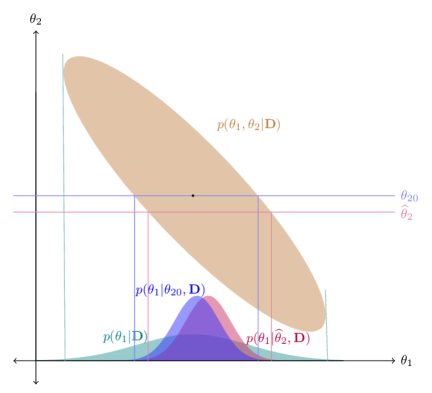
Figure S.1: Heuristics of the two-stage sampler. The brown elliptical region shows the joint posterior $p(\theta_{1},\theta_{2}|{\mathbf{D}})$ of two parameters $\theta_{1}$ and $\theta_{2}$ given data ${\mathbf{D}}$. The light blue curve shows $p(\theta_{1}|{\mathbf{D}})$, the marginal posterior of $\theta_{1}$ given data ${\mathbf{D}}$. The blue curve shows $p(\theta_{1}|\theta_{20},{\mathbf{D}})$, the posterior of $\theta_{1}$, where $\theta_{20}$, the ‘true’ value of $\theta_{2}$, is known. The red curve shows $p(\theta_{1}|\widehat{\theta}_{2},{\mathbf{D}})$, the pseudo-posterior of $\theta_{1}$ given $\widehat{\theta}_{2}$, an estimate of $\theta_{2}$. $p(\theta_{1}|\widehat{\theta}_{2},{\mathbf{D}})$ will be close to $p(\theta_{1}|\theta_{20},{\mathbf{D}})$ when $\widehat{\theta}_{2}$ is close to $\theta_{20}$.

Consider the problem of drawing samples from the posterior $p(\theta_{1},\theta_{2}|{\mathbf{D}})$ of two parameters $\theta_{1}$ and $\theta_{2}$ given data ${\mathbf{D}}$. The basic MCMC sampler iterates between sampling from (A) $p(\theta_{1}|\theta_{2},{\mathbf{D}})$ and (B) $p(\theta_{2}|\theta_{1},{\mathbf{D}})$. If, however, the ‘true’ value of $\theta_{2}$ (in a frequentist sense), say $\theta_{20}$, is known, we only require step (A), which becomes $p(\theta_{1}|\theta_{20},{\mathbf{D}})$. And if we substitute $\theta_{2}$ by a point estimate $\widehat{\theta}_{2}$, step (A) becomes $p(\theta_{1}|\widehat{\theta}_{2},{\mathbf{D}})$. While an uncertainty assessment based on $p(\theta_{1}|\widehat{\theta}_{2},{\mathbf{D}})$ will be overly optimistic compared to that based on the actual marginal posterior $p(\theta_{1}|{\mathbf{D}})$, $p(\theta_{1}|\widehat{\theta}_{2},{\mathbf{D}})$ and $p(\theta_{1}|\theta_{20},{\mathbf{D}})$ will be close when $\widehat{\theta}_{2}$ is close to $\theta_{20}$, and samples drawn from $p(\theta_{1}|\widehat{\theta}_{2},{\mathbf{D}})$ may be used for approximate Bayesian inference on $\theta_{1}$.

The two-stage sampler can also be explained using the following heuristics. Under suitable regularity conditions and considering parametric models (observe that Bayesian nonparametric models are usually large parametric models), the posterior distribution $p(\theta_{1},\theta_{2}|{\mathbf{D}})$ can be approximated by a Gaussian distribution centered at the true value $\mbox{\boldmath$\theta$}_{0}=(\theta_{10},\theta_{20})$ and variance equal to the inverse of the Fisher information matrix ${\mathbf{I}}(\mbox{\boldmath$\theta$}_{0})$. The justification of this argument is usually tedious and follows from Bernstein von-Mises (BvM) theorems. Refer, for example, to Johnstone (2010), Bontemps (2011), Bickel and Kleijn (2012), Spokoiny (2013) and Castillo and Nickl (2014) for recent literature on BvM theorems in nonparametric Bayesian models and growing parametric Bayesian models. For the sake of convenience, let us assume such results are true for $p(\theta_{1},\theta_{2}|{\mathbf{D}})$. Hence the marginal posterior distribution $p(\theta_{1}|{\mathbf{D}})$ is similar to a Gaussian distribution with mean $\theta_{10}$ and variance $[{\mathbf{I}}(\theta_{0})]^{-1}_{11}$, the $(1,1)^{th}$ block of the inverse of ${\mathbf{I}}(\theta_{0})$. Assuming $\widehat{\theta}_{2}$ to be a consistent estimate of $\theta_{20}$, the conditional posterior distribution in step (A) can be approximated by $p(\theta_{1}|\theta_{20},{\mathbf{D}})$ which in turn is similar to a Gaussian distribution centered at $\theta_{10}$ with precision matrix ${\mathbf{I}}(\theta_{10}|\theta_{20})$, the conditional Fisher information matrix assuming $\theta_{20}$ to be known. In classical inference, it is well known that $[{\mathbf{I}}(\theta_{0})]^{-1}_{11}\geq[{\mathbf{I}}(\theta_{10}|\theta_{20})]^{-1}$ in the sense that the difference is non-negative definite, since knowing $\theta_{20}$ results in a higher value of the ‘information’. While confidence intervals based on samples drawn by the two-stage algorithm will be optimistic, the draws will be centered around the true value $\theta_{10}$ and hence may be used for approximate ‘mean’ inference on $\theta_{1}$.

S.5 Comments on the Model for ${{\mathbf{U}}|{\mathbf{X}}}$

As shown in Sarkar, et al. (2014), even in univariate deconvolution settings, due to the nonavailability of precise information about $X$, variations in higher order conditional moments of $(U|X)$ are extremely difficult to capture even in large data sets. Semiparametric approaches that focus separately on the first two moments, namely $E(U|X)=0$ and $\hbox{var}(U|X)$, and the shape of $f_{U|X}$, are thus more efficient than possible fully nonparametric approaches even when the truth closely follows the setup of the nonparametric model. See their Section 4.3. This will certainly remain true in the significantly more difficult multivariate deconvolution problem. In building models for $f_{{\mathbf{U}}|{\mathbf{X}}}$, we may thus concentrate on the class of models that separates the problem of modeling $\hbox{cov}({\mathbf{U}}|{\mathbf{X}})$ from that of modeling the shape and other properties of $f_{{\mathbf{U}}|{\mathbf{X}}}$. Recent advances in covariance regression models, where the covariance of the multivariate regression errors are allowed to vary flexibly with precisely measured and possibly multivariate predictors, provide us with clues about how this may be achieved. However, as we explain in the following section, there are major differences between conditionally varying multivariate regression errors and conditionally varying multivariate measurement errors. As an implication, covariance regression methods may not be exactly appropriate for modeling conditionally varying covariance matrices $\hbox{cov}({\mathbf{U}}|{\mathbf{X}})$ in measurement error settings.

S.5.1 Regression Errors vs Measurement Errors

Consider the problem of flexible modeling of conditionally heteroscedastic regression errors where the response and the covariates are both univariate. Consider also the problem of modeling conditionally heteroscedastic measurement errors in a univariate deconvolution set up. From a modeling perspective, Bayesian hierarchical framework allows us to treat these two problems on par by treating both the covariate in the regression problem and the variable of interest in the deconvolution problem simply as conditioning variables. Of course in the regression problem $X$ is precisely measured, whereas in the deconvolution problem $X$ would be latent, but in either case we are required to flexibly model the density of $(U|X)$ subject to $E(U|X)=0$, where $U$, depending upon the context, denotes either regression or measurement errors. See Figure S.2. Models for regression errors that allow their variance to vary with the values of the covariate (Pati and Dunson, 2013; Pelenis, 2014) can thus be tried as potential candidates for models for univariate conditionally heteroscedastic measurement errors. Conversely, the models for conditionally heteroscedastic univariate measurement errors (Staudenmayer, et al. 2008; Sarkar, et al. 2014) can also be employed to model univariate conditionally heteroscedastic regression errors.

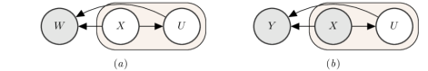
Figure S.2: (a) Dependency structure in a univariate deconvolution model with latent variable of interest $X$, associated measurement errors $U$ and replicates $W$. (b) Dependency structure in a univariate regression model with response $Y$, associated regression errors $U$ and a univariate observed predictor $X$. In both panels, the filled rectangular regions focus on the dependency structures between the conditionally varying errors $U$ and the conditioning variable $X$. The unfilled and the shaded nodes signify latent and observable variables, respectively.

This is not quite true in a multivariate set up. Interpreting the variables of interest ${\mathbf{X}}$ broadly as conditioning variables, one can again loosely connect the problem of modeling conditionally heteroscedastic multivariate measurement errors to the problem of covariance regression (Hoff and Niu, 2012; Fox and Dunson, 2016 etc.), where the goal is to develop models that allow the covariance of multivariate regression errors to vary flexibly with precisely measured and possibly multivariate predictors. In covariance regression problems, the dimension of the regression errors is typically unrelated to the dimension of the predictors. Different components of the regression errors are assumed to be equally influenced by different components of the predictors and hence independent reordering of the components of ${\mathbf{X}}_{i}$ will not change the dependency structure. In multivariate deconvolution problems, in contrast, the $\ell^{th}$ component $U_{ij\ell}$ is the measurement error associated exclusively with $X_{i\ell}$. Here the dimension of ${\mathbf{U}}_{ij}$ is the same as the dimension of ${\mathbf{X}}_{i}$ and any reordering of the components of ${\mathbf{X}}_{i}$ would require that the components of ${\mathbf{U}}_{ij}$ and ${\mathbf{W}}_{ij}$ be also reordered using the same relabeling scheme. See Figure S.3. While different components of the measurement error vectors ${\mathbf{U}}_{ij}$ may be correlated, this exclusive association between $U_{ij\ell}$ and $X_{i\ell}$ implies the plausibility that the dependence of $U_{ij\ell}$ on ${\mathbf{X}}_{i}$ can be explained primarily through $X_{i\ell}$. Figure 7, for instance, suggests strong conditional heteroscedasticity patterns and it is plausible to assume that the conditional variability in $U_{ij\ell}$ can be explained primarily by $X_{i\ell}$ only. The dependency structure of conditionally varying multivariate measurement errors are, therefore, different from that of conditionally varying multivariate regression errors. Additionally, the aforementioned covariance regression approaches all assume multivariate normality of the regression errors. As is well established in the literature, parametric distributional assumptions on the errors can be particularly restrictive in measurement error problems.

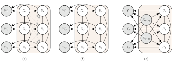
Figure S.3: (a) Dependency structure in a trivariate deconvolution model with latent variable of interest ${\mathbf{X}}=(X_{1},X_{2},X_{3})^{\rm T}$, associated measurement errors ${\mathbf{U}}=(U_{1},U_{2},U_{3})^{\rm T}$ and replicates ${\mathbf{W}}=(W_{1},W_{2},W_{3})^{\rm T}$. The solid black and the dashed gray edges signify strong and weak dependencies, respectively. (b) Dependence relationships in a trivariate deconvolution problem implied by the ‘separable’ measurement error model $({\mathbf{U}}|{\mathbf{X}})={\mathbf{S}}({\mathbf{X}})\mbox{\boldmath$\epsilon$}$ with $\epsilon$ independent of ${\mathbf{X}}$ and ${\mathbf{S}}({\mathbf{X}})=\hbox{diag}\{s_{1}(X_{1}),s_{2}(X_{2}),s_{3}(X_{3})\}$. Unlike panel (a), possible weak relationships between $U_{\ell}$ and $\{X_{m}\}_{m\neq\ell}$ are ignored. (c) Dependency structure in a trivariate regression model with response ${\mathbf{Y}}=(Y_{1},Y_{2},Y_{3})$, associated regression errors ${\mathbf{U}}=(U_{1},U_{2},U_{3})^{\rm T}$ and an observed bivariate predictor ${\mathbf{X}}=(X_{1},X_{2})^{\rm T}$ where ${\mathbf{X}}_{\sigma}=(X_{\sigma(1)},X_{\sigma(2)})^{\rm T}$ denotes arbitrary reordering of ${\mathbf{X}}$. In both panels, the filled rectangular regions focus on the dependency structures between the conditionally varying errors ${\mathbf{U}}$ and the conditioning variable ${\mathbf{X}}$. The unfilled and the shaded nodes signify latent and observable variables, respectively. The directed and the undirected edges represent one-way and two-way relationships, respectively.

These issues preclude direct application of existing covariance regression approaches to model conditionally heteroscedastic multivariate measurement errors. Models for conditionally varying multivariate measurement errors $({\mathbf{U}}|{\mathbf{X}})$ should highlight their unique features, accommodate distributional flexibility, enforce the mean zero restriction and, to be practically effective, should be computationally stable even in the absence of precise information on the conditioning variable ${\mathbf{X}}$.

While we reiterate that, for both modeling and computational reasons, the covariance regression methodology of Fox and Dunson (2016) is not be suitable for our purposes, they still provide clues about how the problems of flexible modeling $\hbox{cov}({\mathbf{U}}|{\mathbf{X}})$ and that of modeling the shape of $f_{{\mathbf{U}}|{\mathbf{X}}}$ can be separated. The following section explains.

S.5.2 Latent Factor Models for Different Covariance Classes

Lemma 6 gives a slightly modified version of Lemma 2.1 of Fox and Dunson (2016).

Lemma 6.

Any conditionally varying covariance matrix $\hbox{cov}({\mathbf{U}}|{\mathbf{X}})=\mbox{\boldmath$\Sigma$}({\mathbf{X}})$ can be represented as $\mbox{\boldmath$\Sigma$}({\mathbf{X}})=\mbox{\boldmath$\Lambda$}({\mathbf{X}})\mbox{\boldmath$\Lambda$}^{\rm T}({\mathbf{X}})$ for some lower triangular matrix $\mbox{\boldmath$\Lambda$}({\mathbf{X}})=((\lambda_{\ell,m}({\mathbf{X}})))$.

Proof.

The proof follows from straightforward application of Cholesky factorization. ∎

Following Lemma 6, introducing a latent factor $\epsilon$, we can write $({\mathbf{U}}|{\mathbf{X}},\mbox{\boldmath$\epsilon$})=\mbox{\boldmath$\Lambda$}({\mathbf{X}})\mbox{\boldmath$\epsilon$}$, that is, $(U_{\ell}|{\mathbf{X}},\mbox{\boldmath$\epsilon$})=\sum_{m=1}^{\ell}\lambda_{\ell,m}({\mathbf{X}})\epsilon_{m}$, with $\mbox{\boldmath$\epsilon$}\perp{\mathbf{X}}$ and $\hbox{cov}(\mbox{\boldmath$\epsilon$})={\mathbf{I}}_{p}$. Completely unrestricted covariance functions can thus be modeled via such latent variable framework by flexibly modeling $\mbox{\boldmath$\Lambda$}({\mathbf{X}})$. $E({\mathbf{U}}|{\mathbf{X}})={\mathbf{0}}$ can be achieved by setting $E(\mbox{\boldmath$\epsilon$})={\mathbf{0}}$.

The general nature of the latent factor formulation having been established, we formulate the subsequent results in terms of additional restrictions on such models. Following the discussion in Section S.5.1, we now focus specifically on covariance functions $\hbox{cov}({\mathbf{U}}|{\mathbf{X}})$ for measurement error problems, where ${\mathbf{U}}$ and ${\mathbf{X}}$ are of the same dimension, each component $U_{\ell}$ of ${\mathbf{U}}$ being related to the corresponding component $X_{\ell}$ of the conditioning vector ${\mathbf{X}}$. We consider first the situation when $(U_{\ell}|{\mathbf{X}},\mbox{\boldmath$\epsilon$})$ depends exclusively on $X_{\ell}$ but not on $\{X_{m}\}_{m\neq\ell}$.

Lemma 7.

Let $({\mathbf{U}}|{\mathbf{X}},\mbox{\boldmath$\epsilon$})=\mbox{\boldmath$\Lambda$}({\mathbf{X}})\mbox{\boldmath$\epsilon$}$, where $\mbox{\boldmath$\Lambda$}({\mathbf{X}})=((\lambda_{\ell,m}({\mathbf{X}})))$ is lower-triangular, $\mbox{\boldmath$\epsilon$}\perp{\mathbf{X}}$ and $\hbox{cov}(\mbox{\boldmath$\epsilon$})={\mathbf{I}}_{p}$. If $(U_{\ell}|{\mathbf{X}},\mbox{\boldmath$\epsilon$})=(U_{\ell}|X_{\ell},\mbox{\boldmath$\epsilon$})$ for all $\ell$, then $\lambda_{\ell,m}({\mathbf{X}})=\lambda_{\ell,m}(X_{\ell})$ for all $\ell,m$.

Proof.

The proof follows trivially by noting that $(U_{\ell}|{\mathbf{X}},\mbox{\boldmath$\epsilon$})=\sum_{m=1}^{\ell}\lambda_{\ell,m}({\mathbf{X}})\epsilon_{m}=(U_{\ell}|X_{\ell},\mbox{\boldmath$\epsilon$})$, if and only if, for all $m\leq\ell$, $\lambda_{\ell,m}({\mathbf{X}})$ is a function of $X_{\ell}$ only. ∎

As an immediate corollary of Lemma 7, the conditional moments $m_{\ell}^{r}({\mathbf{X}})=E(U_{\ell}^{r}|{\mathbf{X}})$ are functions of $X_{\ell}$ only and the conditional cross-moments $m_{\ell,m}^{r,s}({\mathbf{X}})=E(U_{\ell}^{r}U_{m}^{s}|{\mathbf{X}})$ are functions of $X_{\ell}$ and $X_{m}$ only. Modeling variations in the conditional cross-moments is a daunting task in multivariate settings, particularly in the absence of precise information on ${\mathbf{X}}$. The next result allows the cross-moments $m_{\ell,m}^{r,s}({\mathbf{X}})$ to vary with $X_{\ell}$ and $X_{m}$, but assumes the correlations $\hbox{corr}(U_{\ell},U_{m}|{\mathbf{X}})$ to remain constant across ${\mathbf{X}}$.

Lemma 8.

Let $({\mathbf{U}}|{\mathbf{X}},\mbox{\boldmath$\epsilon$})=\mbox{\boldmath$\Lambda$}({\mathbf{X}})\mbox{\boldmath$\epsilon$}$, where $\mbox{\boldmath$\Lambda$}({\mathbf{X}})=((\lambda_{\ell,m}({\mathbf{X}})))$ is lower-triangular, $\mbox{\boldmath$\epsilon$}\perp{\mathbf{X}}$ and $\hbox{cov}(\mbox{\boldmath$\epsilon$})={\mathbf{I}}_{p}$. Also, let $(U_{\ell}|{\mathbf{X}},\mbox{\boldmath$\epsilon$})=(U_{\ell}|X_{\ell},\mbox{\boldmath$\epsilon$})$ for all $\ell$, and $\hbox{corr}(U_{\ell},U_{m}|{\mathbf{X}})$ does not vary with ${\mathbf{X}}$ for all $\ell\neq m$. Then, $\mbox{\boldmath$\Lambda$}({\mathbf{X}})=\mbox{\boldmath$\Lambda$}_{1}({\mathbf{X}}){\mathbf{C}}$ for some diagonal matrix $\mbox{\boldmath$\Lambda$}_{1}({\mathbf{X}})=\hbox{diag}\{\lambda_{1}(X_{1}),\dots,\lambda_{p}(X_{p})\}$ and some lower-triangular matrix ${\mathbf{C}}$.

Proof.

From Lemma 7, we have $\lambda_{\ell,m}({\mathbf{X}})=\lambda_{\ell,m}(X_{\ell})$ for all $\ell,m$, and $\hbox{corr}(U_{\ell},U_{m}|{\mathbf{X}})$ varies with $X_{\ell}$ and $X_{m}$ only. Under the additional assumption of Lemma 8, we first prove that $\lambda_{\ell,m}(X_{\ell})=c_{\ell,m}\lambda_{\ell,\ell}(X_{\ell})$ for some constant $c_{\ell,m}$ for all $m<\ell$ and all $\ell=2,\dots,p$. Without loss of generality, we assume that $\hbox{corr}(U_{\ell},U_{m}|{\mathbf{X}})=r_{\ell,m}\neq 0$ for all $\ell\neq m$. We have

$$\hbox{corr}(U_{1},U_{2}|{\mathbf{X}})=\frac{\lambda_{2,1}(X_{2})}{\{\lambda_{2,1}^{2}(X_{2})+\lambda_{2,2}^{2}(X_{2})\}^{1/2}}=r_{1,2}~{}\Rightarrow~{}\lambda_{2,2}^{2}(X_{2})=\frac{(1-r_{1,2}^{2})}{r_{1,2}^{2}}\lambda_{2,1}^{2}(X_{2}).~{}$$ (S.3)

So the proposition holds true for $\ell=2$. Next, assume that it holds for $\ell=2,\dots,h-1$ for some $h>2$. Also, from (S.3), $\hbox{var}(U_{2}|{\mathbf{X}})=\textstyle\sum_{m=1}^{2}\lambda_{2,m}^{2}(X_{2})=\lambda_{2,1}^{2}(X_{2})/r_{1,2}^{2}$. This is, in fact, more generally true for all $\ell$. For instance, for $\ell=h$,

$$\hbox{corr}(U_{1},U_{h}|{\mathbf{X}})=\frac{\lambda_{h,1}(X_{h})}{\{\sum_{m=1}^{h}\lambda_{h,m}^{2}(X_{h})\}^{1/2}}=r_{1,h}~{}~{}\Rightarrow~{}~{}\sum_{m=2}^{h}\lambda_{h,m}^{2}(X_{h})=\frac{(1-r_{1,h}^{2})}{r_{1,h}^{2}}\lambda_{h,1}^{2}(X_{h})$$

$$~{}~{}\Rightarrow~{}~{}\hbox{var}(U_{h}|{\mathbf{X}})=\textstyle\sum_{m=1}^{h}\lambda_{h,m}^{2}(X_{h})=\lambda_{h,1}^{2}(X_{h})/r_{1,h}^{2}.$$ (S.4)

$$\text{Then,}~{}~{}\hbox{corr}(U_{2},U_{h}|{\mathbf{X}})=\frac{\lambda_{2,1}(X_{2})\lambda_{h,1}(X_{h})+\lambda_{2,2}(X_{2})\lambda_{h,2}(X_{h})}{\{\sum_{m=1}^{2}\lambda_{2,m}^{2}(X_{2})\}^{1/2}\{\sum_{m=1}^{h}\lambda_{h,m}^{2}(X_{h})\}^{1/2}}=r_{2,h}$$

$$~{}~{}\Rightarrow~{}~{}\frac{\lambda_{2,2}(X_{2})\{c_{2,1}\lambda_{h,1}(X_{h})+\lambda_{h,2}(X_{h})\}}{\left|c_{2,1}\lambda_{2,2}(X_{2})\right|\left|\lambda_{h,1}(X_{h})\right|}=\frac{r_{2,h}}{\left|r_{1,2}r_{1,h}\right|}.$$

$$~{}~{}\Rightarrow~{}~{}\lambda_{h,2}(X_{h})=\widetilde{c}_{h,2}\lambda_{h,1}(X_{h})~{}\text{for some constant}~{}\widetilde{c}_{h,2}.$$ (S.5)

$$\text{Next,}~{}~{}\hbox{corr}(U_{3},U_{h}|{\mathbf{X}})=\frac{\sum_{m=1}^{3}\lambda_{3,m}(X_{3})\lambda_{h,m}(X_{h})}{\{\sum_{m=1}^{3}\lambda_{3,m}^{2}(X_{3})\}^{1/2}\{\sum_{m=1}^{h}\lambda_{h,m}^{2}(X_{h})\}^{1/2}}=r_{3,h}$$

$$~{}~{}\Rightarrow~{}~{}\frac{\lambda_{3,3}(X_{3})\{c_{3,1}\lambda_{h,1}(X_{h})+c_{3,2}\widetilde{c}_{h,2}\lambda_{h,1}(X_{h})+\lambda_{h,3}(X_{h})\}}{\left|c_{3,1}\lambda_{3,3}(X_{3})\right|\left|\lambda_{h,1}(X_{h})\right|}=\frac{r_{3,h}}{\left|r_{1,3}r_{1,h}\right|}$$

$$~{}~{}\Rightarrow~{}~{}\lambda_{h,3}(X_{h})=\widetilde{c}_{h,3}\lambda_{h,1}(X_{h})~{}\text{for some constant}~{}\widetilde{c}_{h,3}.$$ (S.6)

$$\text{Finally,}~{}~{}\hbox{corr}(U_{h-1},U_{h}|{\mathbf{X}})=\frac{\sum_{m=1}^{h-1}\lambda_{h-1,m}(X_{h-1})\lambda_{h,m}(X_{h})}{\{\sum_{m=1}^{h-1}\lambda_{h-1,m}^{2}(X_{h-1})\}^{1/2}\{\sum_{m=1}^{h}\lambda_{h,m}^{2}(X_{h})\}^{1/2}}=r_{h-1,h}$$

$$~{}~{}\Rightarrow~{}~{}\frac{\lambda_{h-1,h-1}(X_{h-1})\{c_{h-1,1}\lambda_{h,1}(X_{h})+c_{h-1,2}\widetilde{c}_{h,2}\lambda_{h,1}(X_{h})+\dots+\lambda_{h,h}(X_{h})\}}{\left|c_{h-1,1}\lambda_{h-1,1}(X_{h-1})\right|\left|\lambda_{h,1}(X_{h})\right|}=\frac{r_{h-1,h}}{\left|r_{1,h-1}r_{1,h}\right|}$$

$$~{}~{}\Rightarrow~{}~{}\lambda_{h,h-1}(X_{h})=\widetilde{c}_{h,h-1}\lambda_{h,1}(X_{h})~{}\text{for some constant}~{}\widetilde{c}_{h,h-1}.$$ (S.7)

Combining (S.5), (S.6), (S.7) etc. with (S.4), the proposition follows by principles of mathematical induction. This implies $\mbox{\boldmath$\Lambda$}({\mathbf{X}})=\mbox{\boldmath$\Lambda$}_{1}({\mathbf{X}}){\mathbf{C}}$ where $\mbox{\boldmath$\Lambda$}_{1}({\mathbf{X}})=\hbox{diag}\{\lambda_{1}(X_{1}),\dots,\lambda_{p}(X_{p})\}$ with $\lambda_{\ell}(X_{\ell})=\lambda_{\ell,\ell}(X_{\ell})$ for all $\ell$ and ${\mathbf{C}}=((c_{\ell,m}))$ is a lower triangular matrix with $c_{\ell,\ell}=1$ for all $\ell$. ∎

Under the conditions of Lemma 8, we thus have $\hbox{cov}({\mathbf{U}}|{\mathbf{X}})=\mbox{\boldmath$\Sigma$}({\mathbf{X}})=\mbox{\boldmath$\Lambda$}_{1}({\mathbf{X}})\mbox{\boldmath$\Sigma$}_{1}\mbox{\boldmath$\Lambda$}_{1}^{\rm T}({\mathbf{X}})$ with $\mbox{\boldmath$\Sigma$}_{1}={\mathbf{C}}{\mathbf{C}}^{\rm T}$. Introducing a latent factor $\epsilon$, we can now write $({\mathbf{U}}|{\mathbf{X}},\mbox{\boldmath$\epsilon$})=\mbox{\boldmath$\Lambda$}_{1}({\mathbf{X}})\mbox{\boldmath$\epsilon$}$ with $\mbox{\boldmath$\epsilon$}\perp{\mathbf{X}}$ and $\hbox{cov}(\mbox{\boldmath$\epsilon$})=\mbox{\boldmath$\Sigma$}_{1}$. Due to the diagonal nature of $\mbox{\boldmath$\Lambda$}_{1}({\mathbf{X}})$, each component $\epsilon_{\ell}$ of $\epsilon$ is exclusively associated with the corresponding component $U_{\ell}$ of ${\mathbf{U}}$ and may be treated as a scaled version of $U_{\ell}$. Starting with a general latent factor model framework, with two additional restrictions that are particularly relevant in multivariate measurement error settings, we have now arrived at model (24). The problems of modeling $\hbox{cov}({\mathbf{U}}|{\mathbf{X}})$ and the shape of $f_{{\mathbf{U}}|{\mathbf{X}}}$ can now be achieved by separately modeling $\mbox{\boldmath$\Lambda$}_{1}({\mathbf{X}})$ and $f_{\mbox{\boldmath$\epsilon$}}$. And $E({\mathbf{U}}|{\mathbf{X}})={\mathbf{0}}$ can be achieved by enforcing $E(\mbox{\boldmath$\epsilon$})={\mathbf{0}}$.

S.5.3 Models for ${\mathbf{U}}|{\mathbf{X}}$ and $\hbox{cov}({\mathbf{U}}|{\mathbf{X}})$

In this section, we first revisit the models for conditionally varying measurement errors developed in Section 2.2 of the main paper. A few plausible alternatives and generalizations, the implied covariance structures, their strengths, limitations and connections with the adopted model are also discussed.

The model (24) for conditionally varying measurement errors developed in Section 2.2 of the main paper assumes $({\mathbf{U}}_{ij}|{\mathbf{X}}_{i})={\mathbf{S}}({\mathbf{X}}_{i})\mbox{\boldmath$\epsilon$}_{ij\ell}$ where ${\mathbf{S}}({\mathbf{X}}_{i})=\hbox{diag}\{s_{1}(X_{i1}),\dots,s_{p}(X_{ip})\}$ and $\mbox{\boldmath$\epsilon$}_{ij\ell}$ are distributed independently of ${\mathbf{X}}$ with $E(\mbox{\boldmath$\epsilon$}_{ij})={\mathbf{0}}$. This ‘separability’ of ${\mathbf{X}}_{i}$ and $\mbox{\boldmath$\epsilon$}_{ij}$ allows us to incorporate distributional flexibility and enforce the mean zero restriction using the techniques developed for independent errors in Section 2.2.1 in the main paper. The diagonal structure of ${\mathbf{S}}$ highlights the exclusive associations between $U_{ij\ell}$ and $X_{i\ell}$ but ignores weak dependencies of $U_{ij\ell}$ on $\{X_{im}\}_{m\neq\ell}$. The general of shape of $f_{{\mathbf{U}}|{\mathbf{X}}}$ as well correlations between different components of ${\mathbf{U}}_{ij}$ are inherited from $f_{\mbox{\boldmath$\epsilon$}}$. The associated dependency structure is summarized in Figure S.3(b). The novel two-stage procedure described in Sections S.2 and S.3 produces efficient and numerically stable posterior estimates.

As discussed in Section 2.2.3, the model also arises naturally in multivariate multiplicative measurement error settings ${\mathbf{W}}_{ij}={\mathbf{X}}_{i}\circ\widetilde{\mathbf{U}}_{ij}$ where the errors $\widetilde{\mathbf{U}}_{ij}$ are distributed independently of ${\mathbf{X}}_{i}$ with $E(\widetilde{\mathbf{U}}_{ij})={\mathbf{1}}$. The model can be reformulated as ${\mathbf{W}}_{ij}={\mathbf{X}}_{i}+{\mathbf{U}}_{ij}$, where ${\mathbf{U}}_{ij}={\mathbf{S}}({\mathbf{X}}_{i})\mbox{\boldmath$\epsilon$}_{ij}$, ${\mathbf{S}}({\mathbf{X}}_{i})=\hbox{diag}\{X_{i1},\dots,X_{ip}\}$ and $\mbox{\boldmath$\epsilon$}_{ij}=(\widetilde{\mathbf{U}}_{ij}-1)$ with $E(\mbox{\boldmath$\epsilon$}_{ij})={\mathbf{0}}$. It thus conforms to the conditionally varying additive measurement error model (24) described above.

These results and the ones provided in Section S.5.2 establish the fairly general nature of model (24) and are also informative about cases outside its support. A few such cases that are particularly relevant to measurement error problems and form part of our research aspirations but are not pursued in detail in this article are briefly discussed below.

As informed by Lemma 7, another class that implies $\hbox{var}(U_{ij\ell}|{\mathbf{X}}_{i})=s_{\ell}^{2}(X_{i\ell})$ and allows $\hbox{corr}(U_{ij\ell},U_{ijm}|{\mathbf{X}}_{i})$ to vary with $X_{i\ell}$ and $X_{im}$ is obtained by letting ${\mathbf{U}}_{ij}=\mbox{\boldmath$\Lambda$}({\mathbf{X}}_{i})\mbox{\boldmath$\epsilon$}_{ij}$ with $\mbox{\boldmath$\Lambda$}({\mathbf{X}}_{i})=((\lambda_{\ell,m}(X_{i\ell})))_{\ell=1,m=1}^{p,p}$. The model highlights the exclusive associations between $U_{ij\ell}$ and $X_{i\ell}$ - $\hbox{var}(U_{ij\ell}|{\mathbf{X}}_{i})$ depends on $X_{i\ell}$ and $\hbox{cov}(U_{ij\ell},U_{ijm}|{\mathbf{X}}_{i})$ depends on $X_{i\ell}$ and $X_{im}$. Modeling variations in conditional cross-moments is a daunting task in multivariate settings, more so in the absence of precise information about ${\mathbf{X}}_{i}$. Towards a more parsimonious representation, the off-diagonal elements $\{\lambda_{\ell,m}(X_{i\ell})\}_{\ell\neq m}$ may be shrunk towards zero, resulting in a model that associates each $U_{ij\ell}$ with its own latent factor component $\epsilon_{ij\ell}$. That is, $\mbox{\boldmath$\Lambda$}({\mathbf{X}}_{i})$ should be shrunk towards $\mbox{\boldmath$\Lambda$}_{0}({\mathbf{X}}_{i})=\hbox{diag}\{\lambda_{1,1}(X_{i1}),\dots,\lambda_{p,p}(X_{ip})\}$. This limiting case still allows $\hbox{var}(U_{ij\ell}|{\mathbf{X}}_{i})$ to vary flexibly with $X_{i\ell}$, and $\hbox{cov}(U_{ij\ell},U_{ijm}|{\mathbf{X}})$ to vary with $X_{i\ell}$ and $X_{im}$, but assumes the correlations $\hbox{corr}(U_{ij\ell},U_{ijm}|{\mathbf{X}}_{i})$ to not vary with ${\mathbf{X}}_{i}$.

Another flexible class of models for $({\mathbf{U}}_{ij}|{\mathbf{X}}_{i})$ that conforms to the dependency structure depicted in Figure S.3(a) is obtained by letting ${\mathbf{U}}_{ij}=\mbox{\boldmath$\Lambda$}({\mathbf{X}}_{i})\mbox{\boldmath$\epsilon$}_{ij}$ with $\mbox{\boldmath$\Lambda$}({\mathbf{X}}_{i})=((\lambda_{\ell,m}(X_{im})))_{\ell=1,m=1}^{p,p}$. The implied covariance structure is given by $\hbox{cov}({\mathbf{U}}_{ij}|{\mathbf{X}}_{i})=\mbox{\boldmath$\Sigma$}({\mathbf{X}}_{i})=\mbox{\boldmath$\Lambda$}({\mathbf{X}}_{i})\mbox{\boldmath$\Sigma$}_{\mbox{\boldmath$\epsilon$}}\mbox{\boldmath$\Lambda$}^{\rm T}({\mathbf{X}}_{i})$. Specifically, we have $(U_{ij\ell}|{\mathbf{X}}_{i})=\textstyle\sum_{m}\lambda_{\ell,m}(X_{im})\epsilon_{ijm}$ with

$$\hbox{cov}(U_{ij\ell_{1}},U_{ij\ell_{2}}|{\mathbf{X}}_{i})=\textstyle\sum_{m_{1},m_{2}}\lambda_{\ell_{1},m_{1}}(X_{im_{1}})\lambda_{\ell_{2},m_{2}}(X_{im_{2}})\sigma_{m_{1},m_{2}}$$

$$~{}~{}~{}=\textstyle\lambda_{\ell_{1},\ell_{1}}(X_{i\ell_{1}})\lambda_{\ell_{2},\ell_{2}}(X_{i\ell_{2}})\sigma_{\ell_{1},\ell_{2}}+\sum_{m_{1}\neq\ell_{1},m_{2}\neq\ell_{2}}\lambda_{\ell_{1},m_{1}}(X_{im_{1}})\lambda_{\ell_{2},m_{2}}(X_{im_{2}})\sigma_{m_{1},m_{2}}$$

$$\text{and}~{}~{}~{}\hbox{var}(U_{ij\ell}|{\mathbf{X}}_{i})=\textstyle\lambda_{\ell,\ell}^{2}(X_{i\ell})\sigma_{\ell,\ell}+\sum_{m_{1}\neq\ell,m_{2}\neq\ell}\lambda_{\ell,m_{1}}(X_{im_{1}})\lambda_{\ell,m_{2}}(X_{im_{2}})\sigma_{m_{1},m_{2}}.$$

Ideally, to highlight the exclusive strong association between $U_{ij\ell}$ and $X_{i\ell}$, the diagonal elements of $\mbox{\boldmath$\Lambda$}({\mathbf{X}}_{i})$, namely $\lambda_{\ell,\ell}(X_{i\ell})$, should dominate and the remaining off-diagonal elements $\{\lambda_{\ell,m}(X_{im})\}_{\ell\neq m}$ may be shrunk towards zero. That is, $\mbox{\boldmath$\Lambda$}({\mathbf{X}}_{i})$ should be shrunk towards $\mbox{\boldmath$\Lambda$}_{0}({\mathbf{X}}_{i})=\hbox{diag}\{\lambda_{1,1}(X_{i1}),\dots,\lambda_{p,p}(X_{ip})\}$.

Since measurement error problems are well known to be inherently computationally unstable, it is not clear whether any practical gain in efficiency can be achieved by modeling large number of off-diagonal functions in $\mbox{\boldmath$\Lambda$}({\mathbf{X}}_{i})$ at the expense of significantly increased model complexity. Model (24) considered in this article instead focuses on the special limiting cases with ${\mathbf{S}}({\mathbf{X}}_{i})=\mbox{\boldmath$\Lambda$}_{0}({\mathbf{X}}_{i})$.

Another extension results from mixtures of multiplicative and independent additive errors. In univariate settings, such models were considered in Rocke a Durbin (2001) for studying gene expression levels measured by DNA slides. In multivariate settings, we have ${\mathbf{U}}_{ij}={\mathbf{X}}_{i}\circ\mbox{\boldmath$\epsilon$}_{ij}^{(1)}+\mbox{\boldmath$\epsilon$}_{ij}^{(2)}$, where $\mbox{\boldmath$\epsilon$}_{ij}^{(k)}$, $k=1,2$ are distributed independently of ${\mathbf{X}}_{i}$. With $\hbox{cov}(\mbox{\boldmath$\epsilon$}_{ij}^{(k)})=\mbox{\boldmath$\Sigma$}_{k}=((\sigma_{\ell,m}^{(k)}))_{m=1,\ell=1}^{p,p}$ for $k=1,2$, the implied covariance structure is given by $\hbox{cov}({\mathbf{U}}_{ij}|{\mathbf{X}}_{i})={\mathbf{S}}({\mathbf{X}}_{i})\mbox{\boldmath$\Sigma$}_{1}{\mathbf{S}}({\mathbf{X}}_{i})+\mbox{\boldmath$\Sigma$}_{2}$, where ${\mathbf{S}}({\mathbf{X}}_{i})=\hbox{diag}\{X_{i1},\dots,X_{ip}\}$, as above. The model conforms to the dependency structure of Figure S.3(b) but can not be strictly written as model (24). However, as can be seen from Figure 7, in our motivating nutritional epidemiology application, smaller average consumptions naturally result in more precise 24 hour recalls, the variability approaching 0 as the true consumption approaches 0. Under the assumption of continuity, $\lim_{{\mathbf{X}}\to{\mathbf{0}}}\mbox{\boldmath$\Sigma$}({\mathbf{X}})\to{\mathbf{0}}^{p\times p}$ implies $\mbox{\boldmath$\Sigma$}_{2}={\mathbf{0}}^{p\times p}$, resulting in model (24).

S.5.4 Model Adequacy Checks

In Figure 7 in the main paper, we showed the plots of subject specific means $\overline{W}_{i\ell}$ of the replicates vs the corresponding subject-specific variances $S_{W,i\ell}^{2}$ for each of the four dietary components included in our analysis in Section 7. These plots suggest very strong conditional heteroscedasticity patterns in the measurement errors. If we consider the plots of subject specific means $\overline{W}_{i\ell}$ vs subject specific variances $S_{W,im}^{2}$ for all possible pairs $(\ell,m)$, we will see similar monotone increasing patterns not just for the pairs with $\ell=m$, but in pairs with $\ell\neq m$ too. This can be explained by the high correlation between different components of ${\mathbf{X}}_{i}$, see Figure 8, and does not necessarily imply that the conditional variability in $U_{ij\ell}$ depends on other components of ${\mathbf{X}}_{i}$, not just $X_{i\ell}$. As discussed in the previous subsections, since the $\ell^{th}$ component $U_{ij\ell}$ is the measurement error associated exclusively with $X_{i\ell}$, it is plausible to assume that the conditional variability of $U_{ij\ell}$ can be modeled mostly as a function of $X_{i\ell}$ only.

We present here some diagnostic plots to further validate the practical adequacy of this structural assumption. Figure S.4 shows the plots of $\widehat{X}_{i\ell}$ vs subject specific variances $\widehat{S}_{\epsilon,im}^{2}$ of $\widehat{\epsilon}_{ijm}$, where $\widehat{X}_{i\ell}$ represent the posterior means of $X_{i\ell}$ values and $\widehat{\epsilon}_{ijm}=(W_{ijm}-\widehat{X}_{im})/\widehat{s}_{m}(\widehat{X}_{im})$ represent the corresponding scaled measurement error residuals produced by the univariate submodels for the EATS data set analyzed in Section 7 of the main paper. The figure indicates constant variance of the scaled measurement error residuals $\widehat{\epsilon}_{ij\ell}$ over the entire range of $X_{im}$ values for all $(\ell,m)$ pairs. Nonparametric Eubank-Hart tests of no covariate effect (Eubank and Hart, 1992) applied to $(\widehat{X}_{i\ell},\widehat{S}_{\epsilon,im}^{2})$ for all $(\ell,m)$ pairs (treating $\widehat{X}_{i\ell}$ as the covariate and $\widehat{S}_{\epsilon,im}^{2}$ as the response) produced a minimum Benjamini-Hochberg adjusted p-value of $0.096$, suggesting that there is no residual heteroscedasticity left in $U_{ij\ell}$ after accounting for the variability in $U_{ij\ell}$ that can be sufficiently explained through $X_{i\ell}$ only. See Table S.1. It may thus be concluded that for the EATS data application model (24) developed in Section 2.2.2 of the main paper that implies $\hbox{var}(U_{ij\ell}|{\mathbf{X}}_{i})=s_{\ell}^{2}(X_{i\ell})\hbox{var}(\epsilon_{ij\ell})$ suffices to explain the conditional variability in the measurement errors.

Model (24) also assumed that only the conditional variability of ${\mathbf{U}}_{ij}$ depends on ${\mathbf{X}}_{i}$, and derived other features of ${\mathbf{U}}_{ij}$ like skewness, multimodality, heavy-tails etc. from the scaled errors $\mbox{\boldmath$\epsilon$}_{ij}$. As shown in Sarkar, et al. (2014), even in the much simpler univariate set up, in the absence of precise information on $X_{i\ell}$, variations in other features of $U_{ij\ell}$ for varying values of $X_{i\ell}$, if any, are extremely difficult to detect. More importantly, semiparametric methods that make the multiplicative structural assumption $(U_{ij\ell}|X_{i\ell})=s_{\ell}(X_{i\ell})\epsilon_{ij\ell}$ are highly robust to departures from this assumption and significantly outperform possible nonparametric alternatives that allow all order moments of $U_{ij\ell}$ to vary flexibly with $X_{i\ell}$, not just the conditional variance, even in scenarios where the true data generating process closely conforms to these nonparametric alternatives.

	Panel	p-values	BFN	BH	BY
1	1,1	0.991	1.000	0.991	1.000
2	1,2	0.764	1.000	0.873	1.000
3	1,3	0.251	1.000	0.446	1.000
4	1,4	0.129	1.000	0.446	1.000
5	2,1	0.598	1.000	0.736	1.000
6	2,2	0.266	1.000	0.446	1.000
7	2,3	0.037	0.592	0.197	0.667
8	2,4	0.990	1.000	0.991	1.000
9	3,1	0.224	1.000	0.446	1.000
10	3,2	0.012	0.192	0.096	0.325
11	3,3	0.011	0.176	0.096	0.325
12	3,4	0.497	1.000	0.692	1.000
13	4,1	0.519	1.000	0.692	1.000
14	4,2	0.163	1.000	0.446	1.000
15	4,3	0.279	1.000	0.446	1.000
16	4,4	0.244	1.000	0.446	1.000

Table S.1: The original and adjusted p-values (BFN=Bonferroni, BH=Benjamini-Hochberg, BY=Benjamini-Yekutli) returned by nonparametric Eubank-Hart tests of no covariate effect applied to $(\widehat{X}_{i\ell},\widehat{S}_{\epsilon,im}^{2})$ for all $(\ell,m)$ pairs treating $\widehat{X}_{i\ell}$ as the covariate and $\widehat{S}_{\epsilon,im}^{2}$ as the response. The minimum values corresponding to panel $(3,3)$ are highlighted. See Section S.5.4 and Figure S.4 in the Supplementary Materials for additional details.

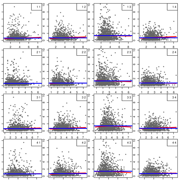
Figure S.4: Panel $(\ell,m)$ shows the plot of estimates $\widehat{X}_{i\ell}$ of $X_{i\ell}$ vs subject specific variances $\widehat{S}_{\epsilon,im}^{2}$ of scaled measurement error residuals $\widehat{\epsilon}_{ijm}$, produced by univariate deconvolution methods. See Section S.5.4 of the Supplementary Materials for additional details. The darker horizontal lines in each panel represent the upper 10% trimmed mean of the subject specific variances $\widehat{S}_{\epsilon,i\ell}^{2}$. The lighter solid lines in each panel represent nonparametric lowess fits.

S.6 Finite vs Infinite Mixture Models

In this article, we modeled the $f_{{\mathbf{X}}}$ and the density of the scaled measurement errors $f_{\mbox{\boldmath$\epsilon$}}$ using mixtures of fixed finite number of multivariate normal kernels. Alternative approaches that escape the need to prespecify the number of mixture components include models with potentially infinite number of mixture components, models induced by Dirichlet processes (Ferguson, 1973; Escobar and West, 1995) being perhaps the most popular among such techniques. Apart from flexibility, one major advantage of such techniques comes from the ability of associated MCMC machinery to perform model selection and model averaging implicitly and semiautomatically. Model averaging is achieved by allowing the number of mixture components to vary from one MCMC iteration to the other. The number of mixture components that is visited the maximum number of times by the sampler then provides a maximum a-posteriori (MAP) estimate of the number of mixture components required to approximate the target density. However, in complicated multivariate set up like ours, MCMC algorithms for such infinite dimensional models become computationally highly intensive. Mixtures based on fixed finite number of components, on the other hand, can greatly reduce computational complexity. Recent studies of asymptotic properties of the posterior of overfitted mixture models (Rousseau and Mengersen, 2011) suggest that mixture models with sufficiently large number of components can perform automatic model selection and model averaging just like infinite dimensional models. Additionally, as the proofs of the results in Section 5 imply, the use of mixture models with fixed finite number of components does not necessarily imply a compromise on the issue of flexibility. The approaches adopted in this article try to take the best from both worlds. Computational burden is reduced by keeping the number of mixture components fixed at some finite values. At the same time, simultaneous semiautomatic model selection and model averaging is achieved by exploiting properties of overfitted mixture models. We elaborate our arguments below, pointing out the close connections and the subtle differences our adopted finite dimensional models have with the aforementioned infinite dimensional alternatives.

S.6.1 Infinite Mixture Models as Limits of Finite Mixture Models

Let $G_{K}=\sum_{k=1}^{K}\pi_{k}\delta_{\theta_{k}}$ with $(\pi_{1},\dots,\pi_{K})\sim\hbox{Dir}(\alpha/K,\dots,\alpha/K)$ and $\theta_{k}\sim H$. Also, let $G_{\infty}\sim\hbox{DP}(\alpha,H)$, a Dirichlet process with concentration parameter $\alpha$ and base measure $H$. Then, $G_{\infty}$ can be represented as $G_{\infty}=\sum_{k=1}^{\infty}\widetilde{\pi}_{k}\delta_{\theta_{k}}$ with $\widetilde{\pi}_{k}=V_{k}\prod_{\ell=1}^{k-1}(1-V_{\ell}),V_{\ell}\sim\hbox{Beta}(1,\alpha)$ and $\theta_{k}\sim H$ (Sethuraman, 1994). As $K\to\infty$, $\int g(\theta)dG_{K}(\theta)\overset{d}{\to}\int g(\theta)dG_{\infty}(\theta)$ for any measurable function $g$ integrable with respect to $H$ (Ishwaran and Zarepour, 2000, 2002).

The finite mixtures of multivariate normal kernels with symmetric Dirichlet priors that we used in this article to model both $f_{{\mathbf{X}}}$ and the density of the scaled measurement errors $f_{\mbox{\boldmath$\epsilon$}}$ have close connections with infinite dimensional Dirichlet process based mixture models. Specifically, taking $g(\theta)=\hbox{MVN}(\mbox{\boldmath$\mu$},\mbox{\boldmath$\Sigma$})$ and appealing to the above result, we have $f_{{\mathbf{X}}}=\sum_{k=1}^{K_{{\mathbf{X}}}}\pi_{{\mathbf{X}},k}\hbox{MVN}(\mbox{\boldmath$\mu$}_{{\mathbf{X}},k},\mbox{\boldmath$\Sigma$}_{{\mathbf{X}},k})\overset{d}{\to}\sum_{k=1}^{\infty}\widetilde{\pi}_{{\mathbf{X}},k}\hbox{MVN}(\mbox{\boldmath$\mu$}_{{\mathbf{X}},k},\mbox{\boldmath$\Sigma$}_{{\mathbf{X}},k})$ as $K_{{\mathbf{X}}}\to\infty$. Our proposed mechanism to enforce the mean zero restriction on $f_{\mbox{\boldmath$\epsilon$}}$ specifically requires a finite dimensional symmetric prior on the mixture probabilities and therefore does not admit a straightforward infinite dimensional extension. But in the limit, as $K_{\mbox{\boldmath$\epsilon$}}\to\infty$, a reformulation of the model results in a complicated multivariate version of the infinite dimensional model of Sarkar, et al. (2014) (See Lemma 5 in Section S.3).

S.6.2 Computational Complexity

The implementation of complex infinite dimensional models, specially the complicated mean restricted model for the scaled errors, will be computationally intensive in a multivariate setting like ours. The computational simplicity of the finite dimensional methods proposed in this article make them particularly suitable for multivariate problems.

In this paragraph, we discuss additional mixing issues that render infinite dimensional models, particularly the ones with non or semiconjugate priors on the component specific parameters (like our MLFA model), unsuitable for multivariate applications. There are two main types of MCMC algorithms for fitting infinite dimensional mixture models - conditional methods and marginal methods. In the conditional scheme, the mixture probabilities are sampled. The mixture labels are then updated independently, conditional on the mixture probabilities. The mixture probabilities in infinite dimensional mixture models can be stochastically ordered. For instance, mixture probabilities in a Dirichlet process mixture model satisfy $E(\widetilde{\pi}_{k})>E(\widetilde{\pi}_{k+1})$ and $\Pr(\widetilde{\pi}_{k}>\widetilde{\pi}_{k+1})>0.5$ for all $k\in\mathbb{N}$. This imposes weak identifiability on the mixture labels resulting in a complicated model space comprising many local modes of varying importance. Different permutations of the mixture labels are not equivalent and exploration of the entire model space becomes important for valid inference. In high dimensional and large data settings it is difficult to achieve even by sophisticated MCMC algorithms with carefully designed label switching moves (Hastie, et al. 2013). The problem can be avoided with marginal methods (Neal, 2000) that integrate out the mixture probabilities and work with the resulting Polya urn scheme, rendering the mixture labels dependent but nonidentifiable. Unfortunately, such integration is possible only when conjugate priors are assigned to the component specific parameters. Typically for infinite dimensional models with non or semiconjugate priors on the component specific parameters, good mixing is thus difficult to achieve, particularly in complicated multivariate setup like ours.

Such issues also plague finite dimensional truncation based approximations to Dirichlet process mixture models where the mixture probabilities are constructed as $\widetilde{\pi}_{k}=V_{k}\prod_{\ell=1}^{k-1}(1-V_{\ell}),V_{\ell}\sim\hbox{Beta}(1,\alpha),k=1,\dots,(K-1)$, and $V_{K}=1$ (Ishwaran and James, 2002) and the mixture components remain weakly identifiable.

On the contrary, the issues of mixing and convergence become much less important for finite mixture models with symmetric priors $(\pi_{1},\dots,\pi_{K})\sim\hbox{Dir}(\alpha/K,\dots,\alpha/K)$ on the mixture probabilities. With $K_{{\mathbf{X}}}$ and $K_{\mbox{\boldmath$\epsilon$}}$ mixture components for the densities $f_{{\mathbf{X}}}$ and $f_{\mbox{\boldmath$\epsilon$}}$, respectively, the posterior is still multimodal but comprises $K_{{\mathbf{X}}}!\times K_{\mbox{\boldmath$\epsilon$}}!$ modal regions that are exact copies of each other. For inference on the overall density or any other functions of interest that are invariant to permutations of the mixture labels, it is only important that the MCMC sampler visits and explores at least one of the modal regions well and label switching (or the lack of it) does not present any problem (Geweke, 2007).

S.6.3 Model Selection and Model Averaging

As mentioned at the beginning of Section S.6, a major advantage of infinite dimensional mixture models is their ability to implicitly and semiautomatically perform model selection and model averaging. Properties of overfitted mixture models can be exploited to achieve the same in finite dimensional models with sufficiently large number of components. Recently Rousseau and Mengersen (2011) studied the asymptotic behavior of the posterior for overfitted mixture models with Dirichlet prior $\hbox{Dir}(\alpha_{1},\dots,\alpha_{K})$ on the mixture probabilities in a measurement error free set up and showed that the hyper parameter $(\alpha_{1},\dots,\alpha_{k})$ strongly influences the way the posterior handles overfitting. In particular, when $\max_{k=1,\dots,K}\alpha_{k}<L/2$, where $L$ denotes the number of parameters specifying the component kernels, the posterior is asymptotically stable and concentrates in regions with empty redundant components. In this article, we chose symmetric Dirichlet priors $\hbox{Dir}(\alpha/K,\dots,\alpha/K)$ on the mixture probabilities to model both the $f_{{\mathbf{X}}}$ and the density of the scaled measurement errors $f_{\mbox{\boldmath$\epsilon$}}$. We set $\alpha_{{\mathbf{X}}}=\alpha_{\mbox{\boldmath$\epsilon$}}=1$ so that the condition $\alpha/K<L/2$ is satisfied for both $f_{{\mathbf{X}}}$ and $f_{\mbox{\boldmath$\epsilon$}}$. In simulation experiments reported in Section 6, the behavior of the posterior was similar to that observed by Rousseau and Mengersen (2011) in measurement error free set up. That is, when $K_{{\mathbf{X}}}$ and $K_{\mbox{\boldmath$\epsilon$}}$ were assigned sufficiently large values, the MCMC chain quickly reached a stable stage where the redundant components became empty. See Figure S.6 in the main article and Figure S.12 and S.13 in the Supplementary Materials for illustrations, where, with some abuse of nomenclature, the $k^{th}$ component is called empty if the associated mixture probability $\pi_{k}\leq 0.05$. Since such overfitted mixture models allow the number of nonempty mixture components to vary from one MCMC iteration to the next, model averaging is automatically achieved. MAP estimates of the numbers of mixture components required to approximate the target densities are given by the numbers of components which are visited the maximum number of times by the MCMC sampler, as in the case of infinite mixture models.

As discussed in the main paper, for the MIW method, when the measurement errors are conditionally heteroscedastic and the true covariance matrices are highly sparse, the strategy usually overestimates the number of non-empty mixture components required to approximate the target densities well. In these cases, the MIW method becomes highly numerically unstable and much larger sample sizes are required for the asymptotic results to hold. See Figure S.5 in the main article for an illustration. This may be regarded more as a limitation of the MIW method than a limitation of the adopted strategy to determine $K_{{\mathbf{X}}}$ and $K_{\mbox{\boldmath$\epsilon$}}$. For the numerically more stable MLFA model, the asymptotic results are valid even for moderate sample sizes and such models are also more robust to overestimation of the number of nonempty clusters.

S.6.4 Model Flexibility

The proofs of the support results presented in Section 5 require that the number of mixture components of the corresponding mixture models be allowed to vary over the set of all positive integers. However, as the technical details of the proofs reveal, the use of mixture models with fixed finite number of components does not necessarily imply a compromise on the issue of flexibility. Indeed, a common recurring idea in the proofs of all these results, including those for the variance functions, is to show that any function coming from the target class can be approximated with any desired level of accuracy by the corresponding finite mixture models provided the models comprise sufficiently large number of mixture components and the function satisfies some fairly minimal regularly conditions. The requirement that the priors on the number of mixture components assign positive probability to all positive integers only helps us reach the final conclusions as immediate consequences. For any given data set of finite size, the number of mixture components required to approximate a target density will always be bounded above by the number of latent or observed variables generated by the target density. For most practical applications the required number would actually be much smaller than the number of variables generated by the target. Even if one applies mixture models that a-priori allow potentially infinitely many mixture components, the posterior will essentially concentrate on a finite set comprising moderately small positive integers. This means that for all practical purposes, solutions based on finite mixture models with fixed but sufficiently large number of mixture components will essentially be as robust as solutions based on their infinite or varying dimensional counterparts while at the same time being significantly less burdensome from a computational viewpoint. The requirement that the priors on the number of mixture components assign positive mass on all positive integers may thus be relegated to the requirement that the priors assign positive mass on sets of the form $\{1,\dots,K\}$, where $K$ is sufficiently large. Posterior computation for such models might be even much more intensive and complex requiring reversible jump moves. Since a mixture model with $K$ components is at least as flexible as a model with $(K-1)$ components, properties of overfitted mixture models discussed in Section S.6.3 allow us to adopt a much simpler strategy. We can simply keep the number of mixture components fixed at sufficiently large values for all MCMC iterations. Carefully chosen priors for the mixture probabilities then result in a posterior that concentrates in regions favoring empty redundant components, essentially eliminating the need to assign any priors on the number of mixture components. We will still need some mechanism, preferably an automated and data adaptive one, to determine what values of $K$ would be sufficiently large. This issue is discussed in the section on hyper-parameter choices in Section S.1.

The discussions of Section S.6 suggest that finite mixture models with sufficiently large number of mixture components and carefully chosen priors for the mixture probabilities can essentially retain the major advantages of infinite dimensional alternatives including flexibility, automated model averaging and model selection while at the same time being computationally much less burdensome, making them our preferred choice for complicated high dimensional problems.

S.7 Proofs of Theoretical Results of Section 5

S.7.1 Proof of Lemma 2

Proof of part 1 of Lemma 2 follows mostly by modifications of the results of Norets and Pelenis (2012). We present here only the proof of part 2 that requires additional modifications along the lines of Pelenis (2014) to accommodate the mean zero restriction on the density of the measurement errors. The first step is to construct finite mixture models of the form

$$f_{m}({\mathbf{z}}|\mbox{\boldmath$\theta$}_{m})=\sum_{k=1}^{m+2}\pi_{m,k}~{}\hbox{MVN}_{p}({\mathbf{z}}|\mbox{\boldmath$\mu$}_{m,k},\mbox{\boldmath$\Sigma$}_{m,k})~{}~{}~{}\text{with}~{}~{}~{}\sum_{k=1}^{m+2}\pi_{m,k}\mbox{\boldmath$\mu$}_{m,k}={\mathbf{0}}$$

that can approximate any given density $f_{0}$ that has mean zero and satisfies Conditions 1 with any desired level of accuracy. The continuity of $f_{m}(\cdot|\mbox{\boldmath$\theta$})$ implies that the KL distance between $f_{0}$ and $f_{m}$ remains small on sufficiently small open neighborhoods around $\mbox{\boldmath$\theta$}_{m}$. Both the MIW and the MLFA priors assign positive probability to open neighborhoods around $\mbox{\boldmath$\theta$}_{m}$. The conclusion of part 2 of Lemma 2 follows since the prior probability of having $(m+2)$ mixture components is also positive for all $m\in\mathbb{N}$.

Lemma 9.

For any $f_{0}\in\widetilde{{\cal F}}_{\mbox{\boldmath$\epsilon$}}$ and $\eta>0$, there exists $\mbox{\boldmath$\theta$}_{m}$ such that $d_{KL}\{f_{0}(\cdot),f_{m}(\cdot|\mbox{\boldmath$\theta$}_{m})\}<\eta$.

Proof.

Let $\{A_{m,k}\}_{k=1}^{m}$ be adjacent cubes with side length $h_{m}$, and $A_{m,0}=\mathbb{R}^{p}-\cup_{k=1}^{m}A_{m,k}$ such that $h_{m}\downarrow 0$ but $\cup_{k=1}^{m}A_{m,k}\uparrow\mathbb{R}^{p}$ as $m\rightarrow\infty$. So $\{A_{m,k}\}_{k=1}^{m}$ becomes finer but $\cup_{k=1}^{m}A_{m,k}$ covers more of $\mathbb{R}^{p}$ as $m$ increases. Additionally, let the partition be constructed in such a way that for all $m$ sufficiently large, if $\mbox{\boldmath$\epsilon$}\in A_{m,0}$, then $C_{r}(\mbox{\boldmath$\epsilon$})\cap A_{m,0}$ contains a hypercube $C_{0}(\mbox{\boldmath$\epsilon$})$ with side length $r/2$ and a vertex at $\epsilon$; and if $\mbox{\boldmath$\epsilon$}\notin A_{m,0}$, then $C_{r}(\mbox{\boldmath$\epsilon$})\cap(\mathbb{R}^{p}-A_{m,0})$ contains a hypercube $C_{1}(\mbox{\boldmath$\epsilon$})$ with side length $r/2$ and a vertex at $\epsilon$. Consider the model

$$f_{m}({\mathbf{z}}) = f_{m}({\mathbf{z}}|\mbox{\boldmath$\theta$}_{m})=\sum_{k=1}^{m+2}\pi_{m,k}~{}\hbox{MVN}_{p}({\mathbf{z}}|\mbox{\boldmath$\mu$}_{m,k},\mbox{\boldmath$\Sigma$}_{m,k}).$$

Set $\pi_{m,k}=\int_{A_{m,k}}f_{0}({\mathbf{z}})d{\mathbf{z}}$ for $k=1,2,\dots,m$ and $\pi_{m,k}=P_{f_{0}}(A_{m,0})/2=\int_{A_{m,k}}f_{0}({\mathbf{z}})d{\mathbf{z}}/2$ for $k=(m+1),(m+2)$. Then $\sum_{k=1}^{m+2}\pi_{m,k}=\int_{\mathbb{R}^{p}}f_{0}({\mathbf{z}})d{\mathbf{z}}=1$. Define $g({\mathbf{d}})=\sum_{k=1}^{m}\pi_{m,k}({\mathbf{c}}_{m,k}+{\mathbf{d}})+\int_{A_{m,0}}{\mathbf{z}}f_{0}({\mathbf{z}})d{\mathbf{z}}$, where ${\mathbf{c}}_{m,k}$ is the center of $A_{m,k}$ for $k=1,2,\dots,m$.

$$g(h_{m}{\mathbf{1}}_{p}/2) = \sum_{k=1}^{m}\pi_{m,k}({\mathbf{c}}_{m,k}+h_{m}{\mathbf{1}}_{p}/2)+\int_{A_{m,0}}{\mathbf{z}}f_{0}({\mathbf{z}})d{\mathbf{z}}$$

$$= \sum_{k=1}^{m}\int_{A_{m,k}}({\mathbf{c}}_{m,k}+h_{m}{\mathbf{1}}_{p}/2)f_{0}({\mathbf{z}})d{\mathbf{z}}+\int_{A_{m,0}}{\mathbf{z}}f_{0}({\mathbf{z}})d{\mathbf{z}}$$

$$\geq \sum_{k=1}^{m}\int_{A_{m,k}}{\mathbf{z}}f_{0}({\mathbf{z}})d{\mathbf{z}}+\int_{A_{m,0}}{\mathbf{z}}f_{0}({\mathbf{z}})d{\mathbf{z}}=\int_{\mathbb{R}^{p}}{\mathbf{z}}f_{0}({\mathbf{z}})d{\mathbf{z}}={\mathbf{0}}.$$

Similarly $g(-h_{m}{\mathbf{1}}_{p}/2)\leq 0$. Since $g(\cdot)$ is continuous, there exists ${\mathbf{d}}_{m}\in[-h_{m}/2,h_{m/2}]^{p}$ such that $g({\mathbf{d}}_{m})={\mathbf{0}}$. Set $\mbox{\boldmath$\mu$}_{m,k}=({\mathbf{c}}_{m,k}+{\mathbf{d}}_{m})$ for $k=1,2,\dots,m$. Also set $\mbox{\boldmath$\mu$}_{m,m+1}=2\int_{A_{m,0}}{\mathbf{z}}f_{0}({\mathbf{z}})d{\mathbf{z}}/\int_{A_{m,0}}f_{0}({\mathbf{z}})d{\mathbf{z}}$ and $\mbox{\boldmath$\mu$}_{m,m+2}={\mathbf{0}}$ when $\int_{A_{m,0}}f_{0}({\mathbf{z}})d{\mathbf{z}}>0$, and $\mbox{\boldmath$\mu$}_{m,0}={\mathbf{0}}$ otherwise. Then $\sum_{k=1}^{m+2}\pi_{m,k}\mbox{\boldmath$\mu$}_{m,k}=g({\mathbf{d}}_{m})={\mathbf{0}}$. Also set $\mbox{\boldmath$\Sigma$}_{m,k}=\sigma_{m}^{2}\hbox{I}_{p}$ for $k=1,2,\dots,m$ with $\sigma_{m}\to 0$, and $\Sigma_{m,m+1}=\Sigma_{m,m+2}=\sigma_{0}^{2}\hbox{I}_{p}$.

Consider a sequence $\{\delta_{m}\}_{m=1}^{\infty}$ satisfying $\delta_{m}>6p^{1/2}h_{m}$ and $\delta_{m}\to 0$. Fix $\mbox{\boldmath$\epsilon$}\in\mathbb{R}^{p}$. Define $C_{\delta_{m}}(\mbox{\boldmath$\epsilon$})=[\mbox{\boldmath$\epsilon$}-\delta_{m}{\mathbf{1}}_{p}/2,\mbox{\boldmath$\epsilon$}+\delta_{m}{\mathbf{1}}_{p}/2]$. For $m$ sufficiently large $C_{\delta_{m}}(\mbox{\boldmath$\epsilon$})\subseteq\cup_{k=1}^{m}A_{m,k}$, $C_{\delta_{m}}(\mbox{\boldmath$\epsilon$})\cap A_{m,0}=\phi$ and the set $\{k:1\leq k\leq m,A_{m,k}\subset C_{\delta_{m}}(\mbox{\boldmath$\epsilon$})\}$ is non-empty. For $k=1,\dots,m$, when $A_{m,k}\subset C_{\delta_{m}}(\mbox{\boldmath$\epsilon$})$, $\pi_{m,k}\geq\inf_{{\mathbf{z}}\in C_{\delta_{m}}(\mbox{\boldmath$\epsilon$})}f_{0}({\mathbf{z}})h_{m}^{p}$. Therefore,

$$f_{m}(\mbox{\boldmath$\epsilon$}) \geq \sum_{\{k:1\leq k\leq m,A_{m,k}\subset C_{\delta_{m}}(\mbox{\boldmath$\epsilon$})\}}~{}\pi_{m,k}~{}\hbox{MVN}_{p}(\mbox{\boldmath$\epsilon$}|\mbox{\boldmath$\mu$}_{m,k},\sigma_{m}^{2}\hbox{I}_{p})$$

$$\geq \inf_{z\in C_{\delta_{m}}(\mbox{\boldmath$\epsilon$})}f_{0}({\mathbf{z}})\sum_{\{k:A_{m,k}\subset C_{\delta_{m}}(\mbox{\boldmath$\epsilon$})\}}h_{m}^{p}~{}\hbox{MVN}_{p}(\mbox{\boldmath$\epsilon$}|{\mathbf{c}}_{m,k}+{\mathbf{d}}_{m},\sigma_{m}^{2}\hbox{I}_{p})$$

$$\geq \inf_{z\in C_{\delta_{m}}(\mbox{\boldmath$\epsilon$})}f_{0}({\mathbf{z}})~{}~{}\left\{1-\frac{6p^{3/2}h_{m}\delta_{m}^{p-1}}{(2\pi)^{p/2}\sigma_{m}^{p}}-\frac{8p\sigma_{m}}{(2\pi)^{1/2}\delta_{m}}\right\},$$

where the last step follows from Lemma 1 and Lemma 2 of Norets and Pelenis (2012). Let $h_{m},\delta_{m},\sigma_{m}$ further satisfy $h_{m}/\sigma_{m}^{p}\to 0,\sigma_{m}/\delta_{m}\to 0$. Then for any $\eta>0$ there exists an $M_{1}$ large enough such that for all $m>M_{1}$

$$f_{m}(\mbox{\boldmath$\epsilon$})\geq\inf_{{\mathbf{z}}\in C_{\delta_{m}}(\mbox{\boldmath$\epsilon$})}f_{0}({\mathbf{z}})\cdot(1-\eta).$$

Without loss of generality, we may assume $f_{0}(\mbox{\boldmath$\epsilon$})>0$. Since $f_{0}(\cdot)$ is continuous and $\delta_{m}\rightarrow 0$, there also exists an $M_{2}$ such that for all $m>M_{2}$ we have $\inf_{{\mathbf{z}}\in C_{\delta_{m}}(\mbox{\boldmath$\epsilon$})}f_{0}({\mathbf{z}})>0$ and

$$\frac{f_{0}(\mbox{\boldmath$\epsilon$})}{\inf_{{\mathbf{z}}\in C_{\delta_{m}}(\mbox{\boldmath$\epsilon$})}f_{0}({\mathbf{z}})}\leq(1+\eta).$$

Therefore, for all $m>\max\{M_{1},M_{2}\}$, we have

$$1\leq\max\left\{1,\frac{f_{0}(\mbox{\boldmath$\epsilon$})}{f_{m}(\mbox{\boldmath$\epsilon$})}\right\}\leq\max\left\{1,\frac{f_{0}(\mbox{\boldmath$\epsilon$})}{\inf_{z\in C_{\delta_{m}}(\mbox{\boldmath$\epsilon$})}f_{0}(z)\cdot(1-\eta)}\right\}\leq\frac{(1+\eta)}{(1-\eta)}.$$

Thus, $\hbox{log}\max\{1,f_{0}(\mbox{\boldmath$\epsilon$})/f_{m}(\mbox{\boldmath$\epsilon$})\}\rightarrow 0$ as $m\rightarrow\infty$. Pointwise convergence is thus established. Next, we will find an integrable upper bound for $\hbox{log}\max\{1,f_{0}(\mbox{\boldmath$\epsilon$})/f_{m}(\mbox{\boldmath$\epsilon$})\}$.

For point wise convergence we can assume $\mbox{\boldmath$\epsilon$}\notin A_{m,0}$ for sufficiently large $m$. But to find integrable upper bound, we have to consider both the cases $\mbox{\boldmath$\epsilon$}\in A_{m,0}$ and $\mbox{\boldmath$\epsilon$}\notin A_{m,0}$. When $\mbox{\boldmath$\epsilon$}\in A_{m,0}$, we have $\hbox{P}_{f_{0}}(A_{m,0})=\int_{A_{m,0}}f_{0}({\mathbf{z}})d{\mathbf{z}}\geq\int_{A_{m,0}\cap C_{r}(\mbox{\boldmath$\epsilon$})}f_{0}({\mathbf{z}})d{\mathbf{z}}\geq\lambda\{A_{m,0}\cap C_{r}(\mbox{\boldmath$\epsilon$})\}\inf_{{\mathbf{z}}\in A_{m,0}\cap C_{r}(\mbox{\boldmath$\epsilon$})}f_{0}({\mathbf{z}})\geq(r/2)^{p}\inf_{{\mathbf{z}}\in C_{r}(\mbox{\boldmath$\epsilon$})}f_{0}({\mathbf{z}})$, since $\lambda\{A_{m,0}\cap C_{r}(\mbox{\boldmath$\epsilon$})\}\geq\lambda\{C_{0}(\mbox{\boldmath$\epsilon$})\}\geq(r/2)^{p}$. Using part 4 of Conditions 1 and Lemma 1 and Lemma 2 of Norets and Pelenis (2012) again, if $\mbox{\boldmath$\epsilon$}\notin A_{m,0}$, for $m$ sufficiently large

$$\sum_{\{k:A_{m,k}\subset C_{r}(\mbox{\boldmath$\epsilon$})\}}h_{m}^{p}~{}\hbox{MVN}_{p}(\mbox{\boldmath$\epsilon$}|\mbox{\boldmath$\mu$}_{m,k},\sigma_{m}^{2}\hbox{I}_{p})\geq\sum_{\{k:A_{m,k}\subset C_{1}(\mbox{\boldmath$\epsilon$})\}}h_{m}^{p}~{}\hbox{MVN}_{p}(\mbox{\boldmath$\epsilon$}|\mbox{\boldmath$\mu$}_{m,k},\sigma_{m}^{2}\hbox{I}_{p})$$

$$\geq\int_{C_{1}(\mbox{\boldmath$\epsilon$})}~{}\hbox{MVN}_{p}({\mathbf{z}}|\mbox{\boldmath$\epsilon$},\sigma_{m}^{2}\hbox{I}_{p})d{\mathbf{z}}-\frac{3p^{3/2}(r/2)^{p-1}h_{m}}{(2\pi)^{p/2}\sigma_{m}^{p}}$$

$$\geq\left\{\frac{1}{2^{p}}-\frac{8p\sigma_{m}}{2^{p}(2\pi)^{1/2}r}-\frac{3p^{3/2}h_{m}r^{p-1}}{2^{p-1}(2\pi)^{p/2}\sigma_{m}^{p}}\right\}\geq\frac{1}{2^{p+1}},$$

This implies

$$f_{m}(\mbox{\boldmath$\epsilon$}) = \sum_{k=1}^{m}P_{f_{0}}(A_{m,k})~{}\hbox{MVN}_{p}(\mbox{\boldmath$\epsilon$}|\mbox{\boldmath$\mu$}_{m,k},\sigma_{m}^{2}\hbox{I}_{p})+\sum_{k=m+1}^{m+2}(1/2)P_{f_{0}}(A_{m,0})~{}\hbox{MVN}_{p}(\mbox{\boldmath$\epsilon$}|\mbox{\boldmath$\mu$}_{m,k},\sigma_{0}^{2}\hbox{I}_{p})$$

$$\geq \sum_{k=1}^{m}P_{f_{0}}(A_{m,k})~{}\hbox{MVN}_{p}(\mbox{\boldmath$\epsilon$}|\mbox{\boldmath$\mu$}_{m,k},\sigma_{m}^{2}\hbox{I}_{p})+(1/2)P_{f_{0}}(A_{m,0})~{}\hbox{MVN}_{p}(\mbox{\boldmath$\epsilon$}|{\mathbf{0}},\sigma_{0}^{2}\hbox{I}_{p})$$

$$\geq \{1-1(\mbox{\boldmath$\epsilon$}\in A_{m,0})\}~{}\inf_{{\mathbf{z}}\in C_{r}(\mbox{\boldmath$\epsilon$})}f_{0}({\mathbf{z}})\sum_{\{k:A_{m,k}\subset C_{r}(\mbox{\boldmath$\epsilon$})\}}\lambda(A_{m,k})~{}\hbox{MVN}_{p}(\mbox{\boldmath$\epsilon$}|\mbox{\boldmath$\mu$}_{m,k},\sigma_{m}^{2}\hbox{I}_{p})$$

$$+~{}1(\mbox{\boldmath$\epsilon$}\in A_{m,0})(1/2)P_{f_{0}}(A_{m,0})~{}\hbox{MVN}_{p}(\mbox{\boldmath$\epsilon$}|{\mathbf{0}},\sigma_{0}^{2}\hbox{I}_{p})$$

$$\geq (1/2)\{1-1(\mbox{\boldmath$\epsilon$}\in A_{m,0})\}~{}\inf_{{\mathbf{z}}\in C_{r}(\mbox{\boldmath$\epsilon$})}f_{0}({\mathbf{z}})$$

$$+~{}1(\mbox{\boldmath$\epsilon$}\in A_{m,0})~{}(1/2)(r/2)^{p}~{}\hbox{MVN}_{p}(\mbox{\boldmath$\epsilon$}|{\mathbf{0}},\sigma_{0}^{2}\hbox{I}_{p})~{}\inf_{{\mathbf{z}}\in C_{r}(\mbox{\boldmath$\epsilon$})}f_{0}({\mathbf{z}})$$

$$\geq (1/2)(r/2)^{p}~{}\hbox{MVN}_{p}(\mbox{\boldmath$\epsilon$}|{\mathbf{0}},\sigma_{0}^{2}\hbox{I}_{p})~{}\inf_{{\mathbf{z}}\in C_{r}(\mbox{\boldmath$\epsilon$})}f_{0}({\mathbf{z}}).$$

The last step followed by choosing $\sigma_{0}^{2}$ large enough so that $(r/2)^{p}\sup_{\mbox{\boldmath$\epsilon$}\in\mathbb{R}^{p}}\hbox{MVN}_{p}(\mbox{\boldmath$\epsilon$}|{\mathbf{0}},\sigma_{0}^{2}\hbox{I}_{p})<(r/2)^{p}~{}\sigma_{0}^{-p}<2^{-(p+1)}<1$. Therefore,

$$\hbox{log}\max\left\{1,\frac{f_{0}(\mbox{\boldmath$\epsilon$})}{f_{m}(\mbox{\boldmath$\epsilon$})}\right\}\leq\hbox{log}\max\left\{1,\frac{f_{0}(\mbox{\boldmath$\epsilon$})}{(1/2)(r/2)^{p}~{}\hbox{MVN}_{p}(\mbox{\boldmath$\epsilon$}|{\mathbf{0}},\sigma_{0}^{2}\hbox{I}_{p})~{}\inf_{{\mathbf{z}}\in C_{r}(\mbox{\boldmath$\epsilon$})}f_{0}({\mathbf{z}})}\right\}$$

$$\leq\hbox{log}\left[\frac{1}{(1/2)(r/2)^{p}~{}\hbox{MVN}_{p}(\mbox{\boldmath$\epsilon$}|{\mathbf{0}},\sigma_{0}^{2}\hbox{I}_{p})}\max\left\{(1/2)(r/2)^{p}~{}\hbox{MVN}_{p}(\mbox{\boldmath$\epsilon$}|{\mathbf{0}},\sigma_{0}^{2}\hbox{I}_{p}),\frac{f_{0}(\mbox{\boldmath$\epsilon$})}{\inf_{{\mathbf{z}}\in C_{r}(\mbox{\boldmath$\epsilon$})}f_{0}({\mathbf{z}})}\right\}\right]$$

$$\leq-\hbox{log}\left\{(1/2)(r/2)^{p}~{}\hbox{MVN}_{p}(\mbox{\boldmath$\epsilon$}|{\mathbf{0}},\sigma_{0}^{2}\hbox{I}_{p})\right\}+\hbox{log}\left\{\frac{f_{0}(\mbox{\boldmath$\epsilon$})}{\inf_{{\mathbf{z}}\in C_{r}(\mbox{\boldmath$\epsilon$})}f_{0}({\mathbf{z}})}\right\}.$$

The first and the second terms are integrable by part 2 and part 3 of Conditions 1, respectively. Since $\int f_{0}(\mbox{\boldmath$\epsilon$})\hbox{log}\{f_{0\mbox{\boldmath$\epsilon$}}/f_{m}(\mbox{\boldmath$\epsilon$})\}d\mbox{\boldmath$\epsilon$}\leq\int f_{0}(\mbox{\boldmath$\epsilon$})\hbox{log}\max\{1,f_{0\mbox{\boldmath$\epsilon$}}/f_{m}(\mbox{\boldmath$\epsilon$})\}d\mbox{\boldmath$\epsilon$}$, the proof of Lemma 9 is completed applying dominated convergence theorem (DCT). ∎

Let $\eta>0$ be given. According to Lemma 9, there exists $\mbox{\boldmath$\theta$}_{m}^{\star}=(\mbox{\boldmath$\pi$}_{1:(m+2)}^{\star},\mbox{\boldmath$\mu$}_{1:(m+2)}^{\star},\mbox{\boldmath$\Sigma$}_{1:(m+2)}^{\star})$ with $\mbox{\boldmath$\Sigma$}_{k}^{\star}=\sigma_{m}^{2\star}\hbox{I}_{p}$ for $k=1,\dots,m$ and $\mbox{\boldmath$\Sigma$}_{k}^{\star}=\sigma_{0}^{2\star}\hbox{I}_{p}$ for $k=(m+1),(m+2)$ such that $d_{KL}\{f_{0}(\cdot),f_{m}(\cdot|\mbox{\boldmath$\theta$}_{m}^{\star})\}<\eta/2$. We have, for any $\mbox{\boldmath$\theta$}_{m}$,

$$\int f_{0}(\mbox{\boldmath$\epsilon$})~{}\hbox{log}\left\{\frac{f_{0}(\mbox{\boldmath$\epsilon$})}{f_{m}(\mbox{\boldmath$\epsilon$}|\mbox{\boldmath$\theta$}_{m})}\right\}d\mbox{\boldmath$\epsilon$}=\int f_{0}(\mbox{\boldmath$\epsilon$})~{}\hbox{log}\left\{\frac{f_{0}(\mbox{\boldmath$\epsilon$})}{f_{m}(\mbox{\boldmath$\epsilon$}|\mbox{\boldmath$\theta$}_{m}^{\star})}\right\}d\mbox{\boldmath$\epsilon$}+\int f_{0}(\mbox{\boldmath$\epsilon$})~{}\hbox{log}\left\{\frac{f_{m}(\mbox{\boldmath$\epsilon$}|\mbox{\boldmath$\theta$}_{m}^{\star})}{f_{m}(\mbox{\boldmath$\epsilon$}|\mbox{\boldmath$\theta$}_{m})}\right\}d\mbox{\boldmath$\epsilon$}.$$

Let the second term in the above expression be denoted by $g(\mbox{\boldmath$\theta$}_{m})$. The priors puts positive mass on arbitrarily small open neighborhoods around $\mbox{\boldmath$\theta$}_{m}^{\star}$. The result will follow if there exists an open neighborhood ${\cal N}(\mbox{\boldmath$\theta$}_{m}^{\star})$ around $\mbox{\boldmath$\theta$}_{m}^{\star}$ such that $\sup_{\mbox{\boldmath$\theta$}_{m}\in{\cal N}(\mbox{\boldmath$\theta$}_{m}^{\star})}g(\mbox{\boldmath$\theta$}_{m})<\eta/2$. Since $g(\mbox{\boldmath$\theta$}_{m}^{\star})=0$, it suffices to show that the function $g(\mbox{\boldmath$\theta$}_{m})$ is continuous at $\mbox{\boldmath$\theta$}_{m}^{\star}$. Now $g(\mbox{\boldmath$\theta$})$ is continuous at $\mbox{\boldmath$\theta$}_{m}^{\star}$ if for every sequence $\{\mbox{\boldmath$\theta$}_{m,n}\}_{n=1}^{\infty}$ with $\mbox{\boldmath$\theta$}_{m,n}\to\mbox{\boldmath$\theta$}_{m}^{\star}$, we have $g(\mbox{\boldmath$\theta$}_{m,n})\to g(\mbox{\boldmath$\theta$}_{m}^{\star})$. For all $\mbox{\boldmath$\epsilon$}\in\mathbb{R}^{p}$, we have $\hbox{log}\{f_{m}(\mbox{\boldmath$\epsilon$}|\mbox{\boldmath$\theta$}_{m,n}^{\star})/f_{m}(\mbox{\boldmath$\epsilon$}|\mbox{\boldmath$\theta$}_{m})\}\to 0$ as $\mbox{\boldmath$\theta$}_{m,n}\to\mbox{\boldmath$\theta$}_{m}^{\star}$. Continuity of $g(\mbox{\boldmath$\theta$}_{m})$ at $\mbox{\boldmath$\theta$}_{m}^{\star}$ will follow from DCT if we can show that $\left|f_{m}(\mbox{\boldmath$\epsilon$}|\mbox{\boldmath$\theta$}_{m}^{\star})/f_{m}(\mbox{\boldmath$\epsilon$}|\mbox{\boldmath$\theta$}_{m,n})\right|$ has an integrable with respect to $f_{0}$ upper bound.

Since $\mbox{\boldmath$\theta$}_{m,n}\to\mbox{\boldmath$\theta$}_{m}^{\star}$, for any arbitrarily small open neighborhood ${\cal N}(\mbox{\boldmath$\theta$}_{m}^{\star})$ around $\mbox{\boldmath$\theta$}_{m}^{\star}$, we must have $\mbox{\boldmath$\theta$}_{m,n}\in{\cal N}(\mbox{\boldmath$\theta$}_{m}^{\star})$ for all $n$ sufficiently large. Let $\mbox{\boldmath$\theta$}_{m}=(\mbox{\boldmath$\pi$}_{1:(m+2)},\mbox{\boldmath$\mu$}_{1:(m+2)},\mbox{\boldmath$\Sigma$}_{1:(m+2)})\in{\cal N}(\mbox{\boldmath$\theta$}_{m}^{\star})$. Since the eigenvalues of a real symmetric matrix depend continuously on the matrix, we must have $(\lambda_{1}(\mbox{\boldmath$\Sigma$}_{k}),\lambda_{p}(\mbox{\boldmath$\Sigma$}_{k}))\subset(\underline{\sigma}_{m}^{2\star},\overline{\sigma}_{m}^{2\star})$ for $k=1,\dots,m$ and $(\lambda_{1}(\mbox{\boldmath$\Sigma$}_{k}),\lambda_{p}(\mbox{\boldmath$\Sigma$}_{k}))\subset(\underline{\sigma}_{0}^{2\star},\overline{\sigma}_{0}^{2\star})$ for $k=(m+1),(m+2)$, where $\underline{\sigma}_{m}^{2\star}<\sigma_{m}^{2\star}<\overline{\sigma}_{m}^{2\star}$ and $\underline{\sigma}_{0}^{2\star}<\sigma_{0}^{2\star}<\overline{\sigma}_{0}^{2\star}$. Let $\underline{\sigma}^{2\star}=\min\{\underline{\sigma}_{m}^{2\star},\underline{\sigma}_{0}^{2\star}\}$ and $\overline{\sigma}^{2\star}=\max\{\overline{\sigma}_{m}^{2\star},\overline{\sigma}_{0}^{2\star}\}$. Then $(\lambda_{1}(\mbox{\boldmath$\Sigma$}_{k}),\lambda_{p}(\mbox{\boldmath$\Sigma$}_{k}))\subset(\underline{\sigma}^{2\star},\overline{\sigma}^{2\star})$ for $k=1,\dots,(m+2)$. Similarly, for some finite $\mu^{\star}$, we must have $\mbox{\boldmath$\mu$}_{m,k}\in(-\mu^{\star}{\mathbf{1}}_{p},\mu^{\star}{\mathbf{1}}_{p})={\cal N}_{\mu^{\star}}$ for $k=1,\dots,(m+2)$. For any real positive definite matrix $\Sigma$, we have ${\mathbf{z}}^{\rm T}\mbox{\boldmath$\Sigma$}^{-1}{\mathbf{z}}\leq\lambda_{1}^{-1}(\mbox{\boldmath$\Sigma$})\left\|{\mathbf{z}}\right\|^{2}$. Therefore, for any $\mbox{\boldmath$\epsilon$}\in\mathbb{R}^{p}$ and for all $k=1,\dots,(m+2)$, we must have $(\mbox{\boldmath$\epsilon$}-\mbox{\boldmath$\mu$}_{m,k})^{\rm T}\mbox{\boldmath$\Sigma$}_{m,k}^{-1}(\mbox{\boldmath$\epsilon$}-\mbox{\boldmath$\mu$}_{m,k})\leq\underline{\sigma}^{-2\star}\{1(\mbox{\boldmath$\epsilon$}\in{\cal N}_{\mu^{\star}})2^{p}\mu^{\star p}+1(\mbox{\boldmath$\epsilon$}\notin{\cal N}_{\mu^{\star}})\left\|\mbox{\boldmath$\epsilon$}+\hbox{sign}(\mbox{\boldmath$\epsilon$})\mu^{\star}\right\|^{2}\}$, where $\hbox{sign}(\mbox{\boldmath$\epsilon$})=\{\hbox{sign}(\epsilon_{1}),\dots,\hbox{sign}(\epsilon_{p})\}^{\rm T}$. Therefore, for any $\mbox{\boldmath$\theta$}_{m}\in{\cal N}(\mbox{\boldmath$\theta$}_{m}^{\star})$, we have

$$[1(\mbox{\boldmath$\epsilon$}\in{\cal N}_{\mu^{\star}})\hbox{MVN}_{p}(2\mu^{\star}{\mathbf{1}}_{p}|{\mathbf{0}},\underline{\sigma}^{2\star}\hbox{I}_{p})+1(\mbox{\boldmath$\epsilon$}\notin{\cal N}_{\mu^{\star}})\hbox{MVN}_{p}\{\mbox{\boldmath$\epsilon$}+\hbox{sign}(\mbox{\boldmath$\epsilon$})\mu^{\star}|{\mathbf{0}},\underline{\sigma}^{2\star}\hbox{I}_{p}\}]/\overline{\sigma}^{\star}$$

$$\leq f_{m}(\mbox{\boldmath$\epsilon$}|\mbox{\boldmath$\theta$}_{m})\leq 1/\underline{\sigma}^{\star}.$$

The upper bound is a constant and the logarithm of the lower bound is integrable since, by part 2 of Conditions 1, the second order moments of $\epsilon$ exist. An $f_{0}$ integrable upper bound for the function $\sup_{\mbox{\boldmath$\theta$}_{m}\in{\cal N}(\mbox{\boldmath$\theta$}_{m}^{\star})}\left|f_{m}(\mbox{\boldmath$\epsilon$}|\mbox{\boldmath$\theta$}_{m})\right|$ thus exists. Finally, DCT applies because

$$\int f_{0}(\mbox{\boldmath$\epsilon$})~{}\left|\hbox{log}\left\{\frac{f_{m}(\mbox{\boldmath$\epsilon$}|\mbox{\boldmath$\theta$}_{m}^{\star})}{f_{m}(\mbox{\boldmath$\epsilon$}|\mbox{\boldmath$\theta$}_{m,n})}\right\}\right|d\mbox{\boldmath$\epsilon$} \leq \sup_{\mbox{\boldmath$\theta$}_{m}\in{\cal N}(\mbox{\boldmath$\theta$}_{m}^{\star})}\int f_{0}(\mbox{\boldmath$\epsilon$})~{}\left|\hbox{log}\left\{\frac{f_{m}(\mbox{\boldmath$\epsilon$}|\mbox{\boldmath$\theta$}_{m}^{\star})}{f_{m}(\mbox{\boldmath$\epsilon$}|\mbox{\boldmath$\theta$}_{m})}\right\}\right|d\mbox{\boldmath$\epsilon$}$$

$$\leq 2\sup_{\mbox{\boldmath$\theta$}_{m}\in{\cal N}(\mbox{\boldmath$\theta$}_{m}^{\star})}\int f_{0}(\mbox{\boldmath$\epsilon$})~{}\left|f_{m}(\mbox{\boldmath$\epsilon$}|\mbox{\boldmath$\theta$}_{m})\right|d\mbox{\boldmath$\epsilon$}.$$

The conclusion of part 2 of Lemma 2 follows since the prior probability of having $(m+2)$ mixture components is positive for all $m\in\mathbb{N}$.

S.7.2 Proof of Lemma 3

Given $q$, let $\Pi_{q}$ denote a prior on $\mathbb{N}_{q}=\{q+1,q+2,\dots\}$ such that $\Pi_{q}(J)>0~{}\forall J\in\mathbb{N}_{q}$. Let $||\cdot||_{2}$ denote the Euclidean norm. Let $\mathbb{R}^{+}=(0,\infty)$. Given $J\sim\Pi_{q}$, also let $\Pi_{\beta|J}$ be a prior on $\mathbb{R}^{+J}$ such that $\Pi_{\beta|J}\{N_{\delta}(\mbox{\boldmath$\beta$}_{0})\}>0$ for any $\delta>0$ and any $\mbox{\boldmath$\beta$}_{0}\in\mathbb{R}^{J}$, where $N_{\delta}(\mbox{\boldmath$\beta$}_{0})=\{\mbox{\boldmath$\beta$}:\mbox{\boldmath$\beta$}\in\mathbb{R}^{+J},||\mbox{\boldmath$\beta$}-\mbox{\boldmath$\beta$}_{0}||_{2}<\delta\}$. Define ${\cal S}_{q,J}=\{v_{s}:v_{s}={\mathbf{B}}_{q,J}\mbox{\boldmath$\beta$}=\sum_{j=1}^{J}b_{q,j}\beta_{j}~{}\hbox{for some}~{}\mbox{\boldmath$\beta$}\in\mathbb{R}^{+J}\}$. Then $\Pi_{{\mathbf{V}}}=\Pi_{q}\times\Pi_{\beta|J}$ is the induced prior on ${\cal S}_{q}=\cup_{J={q+1}}^{\infty}{\cal S}_{q,J}$.

Define $\psi(v_{0},h)=\sup_{X,X^{\prime}\in[A,B],|X-X^{\prime}|\leq h}|v_{0}(X)-v_{0}(X^{\prime})|$. Let $\lfloor\alpha\rfloor=\min\{n:n\in\mathbb{N},n\geq\alpha\}$. For any $X$, $(i)~{}b_{q,j}(X)\geq 0~{}\forall j$, $(ii)~{}\sum_{j=1}^{J}b_{q,j}(X)=1$, $(iii)~{}b_{q,j}$ is positive only inside the interval $[t_{j},t_{j+q+1}]$, and $(iv)$ for $j\in\{(q+1),(q+2),\dots,(q+K)\}$, for any $X\in(t_{j},t_{j+1})$, only $(q+1)$ B-splines $b_{q,j-q}(X),b_{q,j-q+1}(X),\dots,b_{q,j}(X)$ are positive. Using these local support properties of B-splines, the results on page 147 of de Boor (2000) can be modified to show that, for any $v_{0}\in{\cal C}_{+}[A,B]$,

$$\inf_{v_{s}\in{\cal S}_{q,J}}||v_{0}-v_{s}||_{\infty}\leq\lfloor(q+1)/2\rfloor~{}\psi(v_{0},\Delta_{\max})\rightarrow 0~{}~{}\hbox{as}~{}\Delta_{\max}\rightarrow 0.$$

Also, if $q\geq(\alpha-1)$, we can modify the results on page 149 of de Boor (2000) to show that, for any $v\in{\cal C}_{+}^{\alpha}[A,B]$,

$$\inf_{v_{s}\in{\cal S}_{q,J}}||v_{0}-v_{s}||_{\infty} \leq c(q)c(q-1)\dots c(q-\alpha_{0}+1)~{}||v_{0}^{(\alpha_{0})}||_{\infty}~{}\Delta_{\max}^{\alpha_{0}},$$

where $c(q)=\lfloor(q+1)/2\rfloor$. For any two functions $g_{1}$ and $g_{2}$, $\sup|g_{1}g_{2}|\leq\sup|g_{1}|\sup|g_{2}|$. Taking $g_{1}(X,X^{\prime})=\{v_{0}^{(\alpha_{0})}(X)-v_{0}^{(\alpha_{0})}(X^{\prime})\}/(X-X^{\prime})^{(\alpha-\alpha_{0})}$ and $g_{2}(X,X^{\prime})=(X-X^{\prime})^{(\alpha-\alpha_{0})}$, we have $||v_{0}^{(\alpha_{0})}||_{\infty}\leq||v_{0}||_{\alpha}(B-A)^{(\alpha-\alpha_{0})}$. Therefore,

$$\inf_{v_{s}\in{\cal S}_{q,J}}||v_{0}-v_{s}||_{\infty} \leq c(q,\alpha_{0})~{}(B-A)^{(\alpha-\alpha_{0})}~{}||v_{0}||_{\alpha}~{}\Delta_{\max}^{\alpha_{0}}.$$

Furthermore, when the knot points $\{t_{q+1+j}\}_{j=0}^{K}$ are equidistant

$$\inf_{v_{s}\in{\cal S}_{q,J}}||v_{0}-v_{s}||_{\infty}\leq c(q,\alpha_{0})||v_{0}^{(\alpha)}||_{\infty}\frac{(B-A)^{\alpha}}{K^{\alpha_{0}}}\leq c(q,\alpha)||v_{0}||_{\alpha}K^{-\alpha}.$$

Given any $v_{0}\in C_{+}[A,B](\hbox{or}~{}C_{+}^{\alpha}[A,B])$ and $\delta>0$, find $J\in\mathbb{N}_{q}$ and $\mbox{\boldmath$\beta$}_{0}\in\mathbb{R}^{+J}$ such that $||v_{0}-{\mathbf{B}}_{q,J}\mbox{\boldmath$\beta$}_{0}||_{\infty}=\inf_{v_{s}\in{\cal S}_{q,J}}||v_{0}-v_{s}||_{\infty}<\delta/2$. Next consider a neighborhood $N_{\eta}(\mbox{\boldmath$\beta$}_{0})$ such that for any $\mbox{\boldmath$\beta$}\in N_{\eta}(\mbox{\boldmath$\beta$}_{0})$, we have $||{\mathbf{B}}_{q,J}\mbox{\boldmath$\beta$}-{\mathbf{B}}_{q,J}\mbox{\boldmath$\beta$}_{0}||_{\infty}<\delta/2$. Then for any $\mbox{\boldmath$\beta$}\in N_{\eta}(\mbox{\boldmath$\beta$}_{0})$, we have $||{\mathbf{B}}_{q,J}\mbox{\boldmath$\beta$}-v_{0}||_{\infty}\leq||{\mathbf{B}}_{q,J}\mbox{\boldmath$\beta$}-{\mathbf{B}}_{q,J}\mbox{\boldmath$\beta$}_{0}||_{\infty}+||{\mathbf{B}}_{q,J}\mbox{\boldmath$\beta$}_{0}-v_{0}||_{\infty}<\delta$. Also $\Pi_{{\mathbf{V}}}(||v-v_{0}||_{\infty}<\delta)\geq\Pi_{q}(J)~{}\Pi_{\beta|J}\{N_{\eta}(\mbox{\boldmath$\beta$}_{0})\}>0$. Proof of Lemma 3 then follows as a special case taking $\mbox{\boldmath$\beta$}=\exp(\mbox{\boldmath$\xi$})$ and taking $\Pi_{q}$ and $\Pi_{\beta|J}$ to be the priors on $J$ and $\beta$ induced by $P_{0}(K)$ and $P_{0}(\mbox{\boldmath$\xi$}|K,\sigma_{\xi}^{2})$, respectively.

S.7.3 Proof of Lemma 4

We first prove some additional lemmas to used in the proof of Lemma 4.

Lemma 10.

$\Pi_{{\mathbf{V}}}(||v-v_{0}||_{\infty}<\delta)>0~{}\forall\delta>0$ implies that $\Pi_{{\mathbf{V}}}(||g\circ{v}-g\circ{v}_{0}||_{\infty}<\delta)>0~{}\forall\delta>0$ for every continuous function $g:\mathbb{R}\rightarrow\mathbb{R}$.

Proof.

Let ${v}:[A,B]\rightarrow[C_{1},D_{1}]$ and ${v}_{0}:[A,B]\rightarrow[C_{2},D_{2}]$. Then $({v}-{v}_{0}):[A,B]\rightarrow[C_{1}-D_{2},D_{1}-C_{2}]=[C,D]$, say. Then $g:[C,D]\rightarrow\mathbb{R}$ is a uniformly continuous function. Therefore, given any $\delta>0$, there exists a $\eta>0$ such that $|g(Z_{1})-g(Z_{2})|<\delta$ whenever $|Z_{1}-Z_{2}|<\eta$. Now let $||{v}-{v}_{0}||_{\infty}=\sup_{X\in[A,B]}|{v}(X)-{v}_{0}(X)|<\eta$. This implies, for all $X\in[A,B]$, $|{v}(X)-{v}_{0}(X)|<\eta$. Therefore, for all $X\in[A,B]$, $|g\{{v}(X)\}-g\{{v}_{0}(X)\}|<\delta$, and hence $||g\circ{v}-g\circ{v}_{0}||_{\infty}\leq\delta$. Hence the proof. ∎

Corollary 1.

In particular, taking $g(Z)=Z^{1/2}~{}\forall Z>0$ and $g(Z)=0$ otherwise, we have $\Pi_{{\mathbf{V}}}(||v^{1/2}-v_{0}^{1/2}||_{\infty}<\delta)=\Pi_{{\mathbf{V}}}(||s-s_{0}||_{\infty}<\delta)>0~{}\forall\delta>0$ for all ${v}_{0}\in{\cal C}_{+}[A,B](\hbox{or}~{}{\cal C}_{+}^{\alpha}[A,B])$.

Let $P_{\mbox{\boldmath$\epsilon$},K}\{(\mbox{\boldmath$\mu$},\mbox{\boldmath$\Sigma$})|\mbox{\boldmath$\pi$}_{1:K},\mbox{\boldmath$\mu$}_{1:K},\mbox{\boldmath$\Sigma$}_{1:K}\}=\sum_{k=1}^{K}\pi_{k}\delta_{(\mbox{\boldmath$\mu$}_{k},\mbox{\boldmath$\Sigma$}_{k})}(\mbox{\boldmath$\mu$},\mbox{\boldmath$\Sigma$})$, where $\delta_{\mbox{\boldmath$\theta$}}$ denotes a point mass at $\theta$. We have, with the the hyper-parameters implicit, $P_{0}(\mbox{\boldmath$\pi$}_{1:K},\mbox{\boldmath$\mu$}_{1:K},\mbox{\boldmath$\Sigma$}_{1:K})=P_{0\pi}(\mbox{\boldmath$\pi$}_{1:K})P_{0\mu}(\mbox{\boldmath$\mu$}_{1:K}|\mbox{\boldmath$\pi$}_{1:K})P_{0\Sigma}(\mbox{\boldmath$\Sigma$}_{1:K})$. Denoting $P_{\mbox{\boldmath$\epsilon$},K}\{(\mbox{\boldmath$\mu$},\mbox{\boldmath$\Sigma$})|\mbox{\boldmath$\pi$}_{1:K},\mbox{\boldmath$\mu$}_{1:K},\mbox{\boldmath$\Sigma$}_{1:K}\}$ simply by $P_{\mbox{\boldmath$\epsilon$},K}(\mbox{\boldmath$\mu$},\mbox{\boldmath$\Sigma$})$. Let $c$ be a generic for constants that are not of direct interest. For any square matrix ${\mathbf{A}}$ of order $p$, let $\lambda_{1}({\mathbf{A}})\leq\dots\leq\lambda_{p}({\mathbf{A}})$ denote the ordered eigenvalues of ${\mathbf{A}}$. The following lemma proves some properties of $P_{\mbox{\boldmath$\epsilon$},K}$ and $f_{\mbox{\boldmath$\epsilon$}}$.

Lemma 11.

1. $\int\left\|\mbox{\boldmath$\mu$}\right\|_{2}^{2}dP_{\mbox{\boldmath$\epsilon$},K}(\mbox{\boldmath$\mu$},\mbox{\boldmath$\Sigma$})<\infty$ a.s.    2. $\int\lambda_{1}^{-1}(\mbox{\boldmath$\Sigma$})dP_{\mbox{\boldmath$\epsilon$},K}(\mbox{\boldmath$\mu$},\mbox{\boldmath$\Sigma$})<\infty$ a.s.
3. $\int\left|\mbox{\boldmath$\Sigma$}\right|^{-1/2}dP_{\mbox{\boldmath$\epsilon$},K}(\mbox{\boldmath$\mu$},\mbox{\boldmath$\Sigma$})<\infty$ a.s.

Proof.

1. The prior $P_{0\mu}(\mbox{\boldmath$\mu$}_{1:K}|\mbox{\boldmath$\pi$}_{1:K})$ is of the form (23), that is, $P_{0\mu}(\mbox{\boldmath$\mu$}_{1:K}|\mbox{\boldmath$\pi$}_{1:K})=\hbox{MVN}_{Kp}({\mathbf{0}},\mbox{\boldmath$\Sigma$}^{0}-\mbox{\boldmath$\Sigma$}_{1,R}^{0}\mbox{\boldmath$\Sigma$}_{R,R}^{-1}\mbox{\boldmath$\Sigma$}_{R,1}^{0})$, where $\mbox{\boldmath$\Sigma$}^{0}$ is a $Kp\times Kp$ block-diagonal matrix independent of $\mbox{\boldmath$\pi$}_{1:K}$, all $k$ principal blocks of order $p\times p$ being $\mbox{\boldmath$\Sigma$}_{0}$. The matrix $\mbox{\boldmath$\Sigma$}_{1,R}^{0}\mbox{\boldmath$\Sigma$}_{R,R}^{-1}\mbox{\boldmath$\Sigma$}_{R,1}^{0}$ depends on $\mbox{\boldmath$\pi$}_{1:K}$ and is nonnegative definite so that its diagonal elements are all nonnegative. Let $\mbox{\boldmath$\Sigma$}_{0}=((\sigma_{0,ij}))$ and $\mbox{\boldmath$\Sigma$}_{1,R}^{0}\mbox{\boldmath$\Sigma$}_{R,R}^{-1}\mbox{\boldmath$\Sigma$}_{R,1}^{0}=((\sigma_{R,ij}))$. Then, $\int\left\|\mbox{\boldmath$\mu$}_{k}\right\|_{2}^{2}dP_{0\mu}(\mbox{\boldmath$\mu$}_{1:K}|\mbox{\boldmath$\pi$}_{1:K})=\left\{\sum_{j=1}^{p}\sigma_{0,jj}-\sum_{j=(k-1)p+1}^{kp}\sigma_{R,jj}\right\}\leq\sum_{j=1}^{p}\sigma_{0,jj}=\hbox{trace}(\mbox{\boldmath$\Sigma$}_{0})$. Therefore,

$$\int\int\left\|\mbox{\boldmath$\mu$}\right\|_{2}^{2}dP_{\mbox{\boldmath$\epsilon$},K}(\mbox{\boldmath$\mu$},\mbox{\boldmath$\Sigma$})dP_{0}(\mbox{\boldmath$\pi$}_{1:K},\mbox{\boldmath$\mu$}_{1:K},\mbox{\boldmath$\Sigma$}_{1:K})=\sum_{k=1}^{K}\int\pi_{k}\left\|\mbox{\boldmath$\mu$}_{k}\right\|_{2}^{2}dP_{0\mu}(\mbox{\boldmath$\mu$}_{1:K}|\mbox{\boldmath$\pi$}_{1:K})dP_{0\pi}(\mbox{\boldmath$\pi$}_{1:K})$$

$$\leq\hbox{trace}(\mbox{\boldmath$\Sigma$}_{0})<\infty.$$

2. We have $\int\int\lambda_{1}^{-1}(\mbox{\boldmath$\Sigma$})dP_{\mbox{\boldmath$\epsilon$},K}(\mbox{\boldmath$\mu$},\mbox{\boldmath$\Sigma$})dP_{0}(\mbox{\boldmath$\pi$}_{1:K},\mbox{\boldmath$\mu$}_{1:K},\mbox{\boldmath$\Sigma$}_{1:K})=\int\lambda_{1}^{-1}(\mbox{\boldmath$\Sigma$})dP_{0\Sigma}(\mbox{\boldmath$\Sigma$})$.

When $\mbox{\boldmath$\Sigma$}\sim\hbox{IW}_{p}(\nu_{0},\mbox{\boldmath$\Psi$}_{0})$, we have $\mbox{\boldmath$\Psi$}_{0}^{-1/2}\mbox{\boldmath$\Sigma$}^{-1}\mbox{\boldmath$\Psi$}_{0}^{-1/2}\sim\hbox{W}_{p}(\nu_{0},\hbox{I})$ and $\hbox{trace}(\mbox{\boldmath$\Psi$}_{0}^{-1}\mbox{\boldmath$\Sigma$}^{-1})=\hbox{trace}(\mbox{\boldmath$\Psi$}_{0}^{-1/2}\mbox{\boldmath$\Sigma$}^{-1}\mbox{\boldmath$\Psi$}_{0}^{-1/2})\sim\chi^{2}_{p\nu_{0}}$. Here $\hbox{W}_{p}(\nu,\mbox{\boldmath$\Psi$})$ denotes a Wishart distribution with degrees of freedom $\nu$ and mean $\nu\mbox{\boldmath$\Psi$}$. For any two positive semidefinite matrices ${\mathbf{A}}$ and ${\mathbf{B}}$, we have $\lambda_{1}({\mathbf{A}})\hbox{trace}({\mathbf{B}})\leq\hbox{trace}({\mathbf{A}}{\mathbf{B}})\leq\lambda_{p}({\mathbf{A}})\hbox{trace}({\mathbf{B}})$. Therefore, $\lambda_{1}(\mbox{\boldmath$\Psi$}_{0}^{-1})E\{\hbox{trace}(\mbox{\boldmath$\Sigma$}^{-1})\}\leq E\{\hbox{trace}(\mbox{\boldmath$\Psi$}_{0}^{-1}\mbox{\boldmath$\Sigma$}^{-1})\}=p\nu_{0}$. Hence, $\int\lambda_{1}^{-1}(\mbox{\boldmath$\Sigma$})dP_{0\Sigma}(\mbox{\boldmath$\Sigma$})=E\lambda_{p}(\mbox{\boldmath$\Sigma$}^{-1})\leq E\{\hbox{trace}(\mbox{\boldmath$\Sigma$}^{-1})\}<\infty$.

When $\mbox{\boldmath$\Sigma$}=\mbox{\boldmath$\Omega$}+\mbox{\boldmath$\Lambda$}\mbox{\boldmath$\Lambda$}^{\rm T}$ with $\mbox{\boldmath$\Omega$}=\hbox{diag}(\sigma_{1}^{2},\dots,\sigma_{p}^{2})$, we have $\hbox{trace}(\mbox{\boldmath$\Sigma$}^{-1})=\hbox{trace}\{\mbox{\boldmath$\Omega$}^{-1}-\mbox{\boldmath$\Omega$}^{-1}\mbox{\boldmath$\Gamma$}(\hbox{I}_{p}+\mbox{\boldmath$\Gamma$}^{\rm T}\mbox{\boldmath$\Omega$}^{-1}\mbox{\boldmath$\Gamma$})^{-1}\mbox{\boldmath$\Gamma$}^{\rm T}\mbox{\boldmath$\Omega$}^{-1}\}\leq\hbox{trace}(\mbox{\boldmath$\Omega$}^{-1})=\sum_{j=1}^{p}\sigma_{j}^{-2}$, where $\Gamma$ is a $p\times p$ matrix satisfying $\mbox{\boldmath$\Gamma$}\mbox{\boldmath$\Gamma$}^{\rm T}=\mbox{\boldmath$\Lambda$}\mbox{\boldmath$\Lambda$}^{\rm T}$. Thus, $\int\lambda_{1}^{-1}(\mbox{\boldmath$\Sigma$})dP_{0\Sigma}(\mbox{\boldmath$\Sigma$}_{1:K})=E\lambda_{p}(\mbox{\boldmath$\Sigma$}^{-1})\leq E\{\hbox{trace}(\mbox{\boldmath$\Sigma$}^{-1})\}\leq\sum_{j=1}^{p}E\sigma_{j}^{-2}<\infty$ whenever $\sigma_{j}^{2}\sim\hbox{Inv-Ga}(a,b)$ with $a>1$.

3. When $\mbox{\boldmath$\Sigma$}\sim\hbox{IW}_{p}(\nu_{0},\mbox{\boldmath$\Psi$}_{0})$, we have $\lambda_{1}^{p/2}(\mbox{\boldmath$\Psi$}_{0}^{-1})E\{\hbox{trace}(\mbox{\boldmath$\Sigma$}^{-1})\}^{p/2}\leq E\{\hbox{trace}(\mbox{\boldmath$\Psi$}_{0}^{-1}\mbox{\boldmath$\Sigma$}^{-1})\}^{p/2}<\infty$. Hence, $\int\left|\mbox{\boldmath$\Sigma$}\right|^{-1/2}dP_{0\Sigma}(\mbox{\boldmath$\Sigma$})=\int\prod_{j=1}^{p}\lambda_{j}^{1/2}(\mbox{\boldmath$\Sigma$}^{-1})dP_{0\Sigma}(\mbox{\boldmath$\Sigma$})\leq\int\lambda_{p}^{p/2}(\mbox{\boldmath$\Sigma$}^{-1})dP_{0\Sigma}(\mbox{\boldmath$\Sigma$})=E\lambda_{p}^{p/2}(\mbox{\boldmath$\Sigma$}^{-1})\leq E\{\hbox{trace}(\mbox{\boldmath$\Sigma$}^{-1})\}^{p/2}<\infty$.

For any two positive semidefinite matrix ${\mathbf{A}}$ and ${\mathbf{B}}$, we have $\left|{\mathbf{A}}+{\mathbf{B}}\right|\geq\left|{\mathbf{A}}\right|$. Therefore, when $\mbox{\boldmath$\Sigma$}=\mbox{\boldmath$\Omega$}+\mbox{\boldmath$\Lambda$}\mbox{\boldmath$\Lambda$}^{\rm T}$, we have $\int\left|\mbox{\boldmath$\Sigma$}\right|^{-1/2}dP_{0\Sigma}(\mbox{\boldmath$\Sigma$}_{1:K})\leq\int\left|\mbox{\boldmath$\Omega$}\right|^{-1/2}dP_{0\Sigma}(\mbox{\boldmath$\Sigma$}_{1:K})=\int\prod_{j=1}^{p}\sigma_{j}^{-1}dP_{0\Sigma}(\mbox{\boldmath$\Sigma$}_{1:K})=\prod_{j=1}^{p}E\sigma_{j}^{-1}<\infty$, whenever $\sigma_{j}^{2}\sim\hbox{Inv-Ga}(a,b)$ independently. ∎

The following lemma proves a property of $f_{\mbox{\boldmath$\epsilon$}}=\int\int f_{c\mbox{\boldmath$\epsilon$}}(\mbox{\boldmath$\epsilon$}|\mbox{\boldmath$\mu$},\mbox{\boldmath$\Sigma$})dP_{\mbox{\boldmath$\epsilon$},K}(\mbox{\boldmath$\mu$},\mbox{\boldmath$\Sigma$})dP_{0}(K)$. Here $P_{0}(K)$ denotes the prior on $K$, the number of mixture components.

Lemma 12.

Let $f_{0\mbox{\boldmath$\epsilon$}}\in\widetilde{\cal F}_{\mbox{\boldmath$\epsilon$}}$ and $f_{\mbox{\boldmath$\epsilon$}}\sim\Pi_{\mbox{\boldmath$\epsilon$}}$ and ${\mathbf{D}}(\mbox{\boldmath$\tau$})=\hbox{diag}(\tau_{1},\tau_{2},\dots,\tau_{p})$. Then

$$\lim_{\mbox{\boldmath$\tau$}\rightarrow{\mathbf{1}}}\int f_{0\mbox{\boldmath$\epsilon$}}(\mbox{\boldmath$\epsilon$})~{}\hbox{log}\left[\frac{f_{\mbox{\boldmath$\epsilon$}}(\mbox{\boldmath$\epsilon$})}{\left|{\mathbf{D}}(\mbox{\boldmath$\tau$})\right|^{-1}f_{\mbox{\boldmath$\epsilon$}}\{{\mathbf{D}}(\mbox{\boldmath$\tau$})\mbox{\boldmath$\epsilon$}\}}\right]~{}d\mbox{\boldmath$\epsilon$}=0.$$

Proof.

We have $\left|{\mathbf{D}}(\mbox{\boldmath$\tau$})\right|^{-1}f_{c\mbox{\boldmath$\epsilon$}}\{{\mathbf{D}}(\mbox{\boldmath$\tau$})\mbox{\boldmath$\epsilon$}\}\to f_{c\mbox{\boldmath$\epsilon$}}(\mbox{\boldmath$\epsilon$})$ as $\mbox{\boldmath$\tau$}\to{\mathbf{1}}$. Since $\mbox{\boldmath$\tau$}\rightarrow{\mathbf{1}}$, without loss of generality, we may assume $\left|{\mathbf{D}}(\mbox{\boldmath$\tau$})\right|>1/2$. Define $c=\int\left|\mbox{\boldmath$\Sigma$}\right|^{-1/2}dP_{\mbox{\boldmath$\epsilon$},K}(\mbox{\boldmath$\mu$},\mbox{\boldmath$\Sigma$})$. Then $c<\infty$. Also $\int\left|{\mathbf{D}}(\mbox{\boldmath$\tau$})\right|^{-1}f_{c\mbox{\boldmath$\epsilon$}}\{{\mathbf{D}}(\mbox{\boldmath$\tau$})\mbox{\boldmath$\epsilon$}|\mbox{\boldmath$\theta$}\}dP_{\mbox{\boldmath$\epsilon$},K}(\mbox{\boldmath$\mu$},\mbox{\boldmath$\Sigma$})\leq\int 2(2\pi)^{-p/2}\left|\mbox{\boldmath$\Sigma$}\right|^{-1/2}dP_{\mbox{\boldmath$\epsilon$},K}(\mbox{\boldmath$\mu$},\mbox{\boldmath$\Sigma$})<2c<\infty$. Applying DCT, $\left|{\mathbf{D}}(\mbox{\boldmath$\tau$})\right|^{-1}f_{\mbox{\boldmath$\epsilon$}}\{{\mathbf{D}}(\mbox{\boldmath$\tau$})\mbox{\boldmath$\epsilon$}\}\rightarrow f_{\mbox{\boldmath$\epsilon$}}(\mbox{\boldmath$\epsilon$})$ as $\mbox{\boldmath$\tau$}\rightarrow{\mathbf{1}}$. Therefore, for any $\mbox{\boldmath$\epsilon$}\in\mathbb{R}$,

$$\hbox{log}\left[\frac{f_{\mbox{\boldmath$\epsilon$}}(\mbox{\boldmath$\epsilon$})}{\left|{\mathbf{D}}(\mbox{\boldmath$\tau$})\right|^{-1}f_{\mbox{\boldmath$\epsilon$}}\{{\mathbf{D}}(\mbox{\boldmath$\tau$})\mbox{\boldmath$\epsilon$}\}}\right]\rightarrow 0~{}~{}~{}\hbox{as}~{}\mbox{\boldmath$\tau$}\rightarrow{\mathbf{1}}.$$

To find an integrable with respect to $f_{0\mbox{\boldmath$\epsilon$}}$ upper bound for $\hbox{log}\left[\left|{\mathbf{D}}(\mbox{\boldmath$\tau$})\right|f_{\mbox{\boldmath$\epsilon$}}(\mbox{\boldmath$\epsilon$})/f_{\mbox{\boldmath$\epsilon$}}\{{\mathbf{D}}(\mbox{\boldmath$\tau$})\mbox{\boldmath$\epsilon$}\}\right]$, we use Lemma 11. To do so, we can ignore the prior $P_{0}(K)$ since the upper bounds obtained in Lemma 11 do not depend on the specific choice of $K$. We have, using part 3 of Lemma 11,

$$\int\left|\mbox{\boldmath$\Sigma$}\right|^{-1/2}\exp\left[-\frac{1}{2}\{{\mathbf{D}}(\mbox{\boldmath$\tau$})\mbox{\boldmath$\epsilon$}-\mbox{\boldmath$\mu$}\}^{\rm T}\mbox{\boldmath$\Sigma$}^{-1}\{{\mathbf{D}}(\mbox{\boldmath$\tau$})\mbox{\boldmath$\epsilon$}-\mbox{\boldmath$\mu$}\}\right]dP_{\mbox{\boldmath$\epsilon$},K}(\mbox{\boldmath$\mu$},\mbox{\boldmath$\Sigma$})$$

$$\leq\int\left|\mbox{\boldmath$\Sigma$}\right|^{-1/2}dP_{\mbox{\boldmath$\epsilon$},K}(\mbox{\boldmath$\mu$},\mbox{\boldmath$\Sigma$})\leq c.$$

Since $\mbox{\boldmath$\tau$}\rightarrow{\mathbf{1}}$, without loss of generality we may also assume $\tau_{k}<2$ for all $k$. Therefore,

$$|\hbox{log}~{}f_{\mbox{\boldmath$\epsilon$}}\{{\mathbf{D}}(\mbox{\boldmath$\tau$})\mbox{\boldmath$\epsilon$}\}|$$

$$\leq\hbox{log}(2\pi)^{p/2}+\left|\hbox{log}\int\left|\mbox{\boldmath$\Sigma$}\right|^{-1/2}\exp\left[-\frac{1}{2}\{{\mathbf{D}}(\mbox{\boldmath$\tau$})\mbox{\boldmath$\epsilon$}-\mbox{\boldmath$\mu$}\}^{\rm T}\mbox{\boldmath$\Sigma$}^{-1}\{{\mathbf{D}}(\mbox{\boldmath$\tau$})\mbox{\boldmath$\epsilon$}-\mbox{\boldmath$\mu$}\}\right]dP_{\mbox{\boldmath$\epsilon$},K}(\mbox{\boldmath$\mu$},\mbox{\boldmath$\Sigma$})\right|$$

$$\leq\hbox{log}(2\pi)^{p/2}+|\hbox{log}~{}c|$$

$$~{}~{}~{}~{}~{}~{}~{}~{}~{}~{}~{}-\hbox{log}\int c^{-1}\left|\mbox{\boldmath$\Sigma$}\right|^{-1/2}\exp\left[-\frac{1}{2}\{{\mathbf{D}}(\mbox{\boldmath$\tau$})\mbox{\boldmath$\epsilon$}-\mbox{\boldmath$\mu$}\}^{\rm T}\mbox{\boldmath$\Sigma$}^{-1}\{{\mathbf{D}}(\mbox{\boldmath$\tau$})\mbox{\boldmath$\epsilon$}-\mbox{\boldmath$\mu$}\}\right]dP_{\mbox{\boldmath$\epsilon$},K}(\mbox{\boldmath$\mu$},\mbox{\boldmath$\Sigma$})$$

$$\leq\hbox{log}\{c(2\pi)^{p/2}\}+|\hbox{log}~{}c|$$

$$~{}~{}~{}~{}~{}~{}~{}~{}~{}~{}~{}+\frac{1}{2}\int\hbox{log}\left|\mbox{\boldmath$\Sigma$}\right|dP_{\mbox{\boldmath$\epsilon$},K}(\mbox{\boldmath$\mu$},\mbox{\boldmath$\Sigma$})+\frac{1}{2}\int\{{\mathbf{D}}(\mbox{\boldmath$\tau$})\mbox{\boldmath$\epsilon$}-\mbox{\boldmath$\mu$}\}^{\rm T}\mbox{\boldmath$\Sigma$}^{-1}\{{\mathbf{D}}(\mbox{\boldmath$\tau$})\mbox{\boldmath$\epsilon$}-\mbox{\boldmath$\mu$}\}dP_{\mbox{\boldmath$\epsilon$},K}(\mbox{\boldmath$\mu$},\mbox{\boldmath$\Sigma$})$$

$$\leq\hbox{log}\{c(2\pi)^{p/2}\}+|\hbox{log}~{}c|$$

$$~{}~{}~{}~{}~{}~{}~{}~{}~{}~{}~{}+\frac{1}{2}\int\hbox{log}\left|\mbox{\boldmath$\Sigma$}\right|dP_{\mbox{\boldmath$\epsilon$},K}(\mbox{\boldmath$\mu$},\mbox{\boldmath$\Sigma$})+\frac{1}{2}\int\left\|{\mathbf{D}}(\mbox{\boldmath$\tau$})\mbox{\boldmath$\epsilon$}-\mbox{\boldmath$\mu$}\right\|_{2}^{2}\lambda_{1}^{-1}(\mbox{\boldmath$\Sigma$})dP_{\mbox{\boldmath$\epsilon$},K}(\mbox{\boldmath$\mu$},\mbox{\boldmath$\Sigma$})$$

$$\leq\hbox{log}\{c(2\pi)^{p/2}\}+|\hbox{log}~{}c|$$

$$~{}~{}~{}~{}~{}~{}~{}~{}~{}~{}~{}+\frac{1}{2}\int\hbox{log}\left|\mbox{\boldmath$\Sigma$}\right|dP_{\mbox{\boldmath$\epsilon$},K}(\mbox{\boldmath$\mu$},\mbox{\boldmath$\Sigma$})+\int\{\left\|{\mathbf{D}}(\mbox{\boldmath$\tau$})\mbox{\boldmath$\epsilon$}\right\|_{2}^{2}+\left\|\mbox{\boldmath$\mu$}\right\|_{2}^{2}\}\lambda_{1}^{-1}(\mbox{\boldmath$\Sigma$})dP_{\mbox{\boldmath$\epsilon$},K}(\mbox{\boldmath$\mu$},\mbox{\boldmath$\Sigma$})$$

$$\leq\hbox{log}\{c(2\pi)^{p/2}\}+|\hbox{log}~{}c|+\frac{1}{2}\int\hbox{log}\left|\mbox{\boldmath$\Sigma$}\right|dP_{\mbox{\boldmath$\epsilon$},K}(\mbox{\boldmath$\mu$},\mbox{\boldmath$\Sigma$})$$

$$~{}~{}~{}~{}~{}~{}~{}~{}~{}~{}~{}+\left\|2\mbox{\boldmath$\epsilon$}\right\|_{2}^{2}\int\lambda_{1}^{-1}(\mbox{\boldmath$\Sigma$})dP_{\mbox{\boldmath$\epsilon$},K}(\mbox{\boldmath$\mu$},\mbox{\boldmath$\Sigma$})+\int\left\|\mbox{\boldmath$\mu$}\right\|_{2}^{2}dP_{\mbox{\boldmath$\epsilon$},K}(\mbox{\boldmath$\mu$},\mbox{\boldmath$\Sigma$})\int\lambda_{1}^{-1}(\mbox{\boldmath$\Sigma$})dP_{\mbox{\boldmath$\epsilon$},K}(\mbox{\boldmath$\mu$},\mbox{\boldmath$\Sigma$}),$$

where the third step followed from application of Jensen’s inequality on $g(Z)=-\hbox{log}~{}Z$. The regularity assumptions on $f_{0\mbox{\boldmath$\epsilon$}}$ and Lemma 11 imply that the RHS above is $f_{0\mbox{\boldmath$\epsilon$}}$ integrable. The conclusion of Lemma 12 follows from an application of DCT again. ∎

To prove Lemma 4, let $f_{{\mathbf{U}}|{\mathbf{S}}}$ denote the density of ${\mathbf{U}}={\mathbf{S}}({\mathbf{X}})\mbox{\boldmath$\epsilon$}$, where ${\mathbf{S}}=\hbox{diag}(s_{1},\dots,s_{p})$. Then $f_{{\mathbf{U}}|{\mathbf{X}}}=f_{{\mathbf{U}}|{\mathbf{S}}({\mathbf{X}})}$. We have $f_{{\mathbf{U}}|{\mathbf{S}}}({\mathbf{U}})=\left|{\mathbf{S}}\right|^{-1}f_{\mbox{\boldmath$\epsilon$}}({\mathbf{S}}^{-1}{\mathbf{U}})$. This implies

$$\int f_{0{\mathbf{U}}|{\mathbf{S}}_{0}}({\mathbf{U}})\hbox{log}\frac{f_{0{\mathbf{U}}|{\mathbf{S}}_{0}}({\mathbf{U}})}{f_{{\mathbf{U}}|{\mathbf{S}}}({\mathbf{U}})}d{\mathbf{U}}=\int f_{0{\mathbf{U}}|{\mathbf{S}}_{0}}({\mathbf{U}})\hbox{log}\frac{f_{0{\mathbf{U}}|{\mathbf{S}}_{0}}({\mathbf{U}})}{f_{{\mathbf{U}}|{\mathbf{S}}_{0}}({\mathbf{U}})}d{\mathbf{U}}+\int f_{0{\mathbf{U}}|{\mathbf{S}}_{0}}({\mathbf{U}})\hbox{log}\frac{f_{{\mathbf{U}}|{\mathbf{S}}_{0}}({\mathbf{U}})}{f_{{\mathbf{U}}|{\mathbf{S}}}({\mathbf{U}})}d{\mathbf{U}}$$

$$=\int f_{0\mbox{\boldmath$\epsilon$}}(\mbox{\boldmath$\epsilon$})\hbox{log}\frac{f_{0\mbox{\boldmath$\epsilon$}}(\mbox{\boldmath$\epsilon$})}{f_{\mbox{\boldmath$\epsilon$}}(\mbox{\boldmath$\epsilon$})}d\mbox{\boldmath$\epsilon$}+\int f_{0\mbox{\boldmath$\epsilon$}}(\mbox{\boldmath$\epsilon$})\hbox{log}\frac{f_{\mbox{\boldmath$\epsilon$}}(\mbox{\boldmath$\epsilon$})}{\left|{\mathbf{S}}\right|^{-1}\left|{\mathbf{S}}_{0}\right|f_{\mbox{\boldmath$\epsilon$}}({\mathbf{S}}^{-1}{\mathbf{S}}_{0}\mbox{\boldmath$\epsilon$})}d\mbox{\boldmath$\epsilon$}.$$

Let $\delta>0$ be given. By part 2 of Lemma 2, $\Pi_{\mbox{\boldmath$\epsilon$}}\{f_{\mbox{\boldmath$\epsilon$}}:d_{KL}(f_{0\mbox{\boldmath$\epsilon$}},f_{\mbox{\boldmath$\epsilon$}})<\delta/2\}>0$. Let ${\mathbf{s}}=(s_{1},\dots,s_{p})^{\rm T}$ and ${\mathbf{s}}_{0}=(s_{01},\dots,s_{0p})^{\rm T}$. By Lemma 12, there exists $\eta>0$ such that $\left\|{\mathbf{s}}_{0}-{\mathbf{s}}\right\|_{\infty}<\eta$ implies $\int f_{0\mbox{\boldmath$\epsilon$}}(\mbox{\boldmath$\epsilon$})~{}\hbox{log}[f_{\mbox{\boldmath$\epsilon$}}(\mbox{\boldmath$\epsilon$})/\{\left|{\mathbf{S}}\right|^{-1}\left|{\mathbf{S}}_{0}\right|f_{\mbox{\boldmath$\epsilon$}}({\mathbf{S}}^{-1}{\mathbf{S}}_{0}\mbox{\boldmath$\epsilon$})\}]~{}d\mbox{\boldmath$\epsilon$}<\delta/2$ for every $f_{\mbox{\boldmath$\epsilon$}}\sim\Pi_{\mbox{\boldmath$\epsilon$}}$. Using a straightforward multivariate extension of Corollary 1, we have $\Pi_{{\mathbf{V}}}(||{\mathbf{s}}_{0}-{\mathbf{s}}||_{\infty}<\eta)>0$. Combining these results, $\Pi_{{\mathbf{U}}|{\mathbf{V}}}\{\sup_{{\mathbf{X}}\in{\cal X}}d_{KL}(f_{0{\mathbf{U}}|{\mathbf{X}}},f_{{\mathbf{U}}|{\mathbf{X}}})<\delta\}\geq\Pi_{\mbox{\boldmath$\epsilon$}}\{d_{KL}(f_{0\mbox{\boldmath$\epsilon$}},f_{\mbox{\boldmath$\epsilon$}})<\delta/2\}~{}\Pi_{{\mathbf{V}}}(||{{\mathbf{s}}}_{0}-{\mathbf{s}}||_{\infty}<\eta)>0$. Hence the proof of part 2 of Lemma 4.

Part 1 of Lemma 4 follows trivially from part 2 of Lemma 4 since $||{\mathbf{s}}_{0}-{\mathbf{s}}||_{\infty}<\eta$ implies $\left\|{\mathbf{s}}_{0}({\mathbf{X}})-{\mathbf{s}}({\mathbf{X}})\right\|_{\infty}<\eta$ for any ${\mathbf{X}}\in{\cal X}$.

To prove part 3 of Lemma 4, note that

$$d_{KL}(f_{0,{\mathbf{X}},{\mathbf{U}}},f_{{\mathbf{X}},{\mathbf{U}}})=\int_{{\cal X}\times\mathbb{R}^{p}}f_{0,{\mathbf{U}}|{\mathbf{X}}}({\mathbf{U}}|{\mathbf{X}})f_{0,{\mathbf{X}}}({\mathbf{X}})~{}\hbox{log}\frac{f_{0,{\mathbf{U}}|{\mathbf{X}}}({\mathbf{U}}|{\mathbf{X}})f_{0,{\mathbf{X}}}({\mathbf{X}})}{f_{{\mathbf{U}}|{\mathbf{X}}}({\mathbf{U}}|{\mathbf{X}})f_{\mathbf{X}}({\mathbf{X}})}d{\mathbf{X}}d{\mathbf{U}}$$

$$= \int_{{\cal X}}f_{0,{\mathbf{X}}}({\mathbf{X}})\int_{\mathbb{R}^{p}}f_{0,{\mathbf{U}}|{\mathbf{X}}}({\mathbf{U}}|{\mathbf{X}})~{}\hbox{log}\frac{f_{0,{\mathbf{U}}|{\mathbf{X}}}({\mathbf{U}}|{\mathbf{X}})}{f_{{\mathbf{U}}|{\mathbf{X}}}({\mathbf{U}}|{\mathbf{X}})}d{\mathbf{U}}d{\mathbf{X}}+\int_{{\cal X}}f_{0,{\mathbf{X}}}({\mathbf{X}})~{}\hbox{log}\frac{f_{0,{\mathbf{X}}}({\mathbf{X}})}{f_{{\mathbf{X}}}({\mathbf{X}})}d{\mathbf{X}}$$

$$\leq \sup_{{\mathbf{X}}\in{\cal X}}d_{KL}\{f_{0,{\mathbf{U}}|{\mathbf{X}}}({\mathbf{U}}|{\mathbf{X}}),f_{{\mathbf{U}}|{\mathbf{X}}}({\mathbf{U}}|{\mathbf{X}})\}+d_{KL}(f_{0{\mathbf{X}}},f_{{\mathbf{X}}}).$$

Part 3 of Lemma 4 now follows from part 2 of Lemma 4 and part 1 of Lemma 2.

S.7.4 Proof of Theorem 1

Let $d_{H}(f_{0},f)=[\int\{f_{0}^{1/2}({\mathbf{Z}})-f^{1/2}({\mathbf{Z}})\}^{2}d{\mathbf{Z}}]^{1/2}$ denote the Hellinger distance between any two densities $f_{0}$ and $f$. From Chapter 1 of Ghosh and Ramamoorthi (2010), we have

$$d_{H}^{2}(f_{0},f)\leq||f_{0}-f||_{1}\leq 2~{}d_{KL}^{1/2}(f_{0},f).$$ (S.8)

Using (S.8), we have,

$$||f_{0{\mathbf{W}}}-f_{{\mathbf{W}}}||_{1}=\int|f_{0{\mathbf{W}}}({\mathbf{W}})-f_{{\mathbf{W}}}({\mathbf{W}})|d{\mathbf{W}}$$

$$= \int\left|\int f_{0{\mathbf{X}}}({\mathbf{X}})f_{0{\mathbf{W}}|{\mathbf{X}}}({\mathbf{W}})d{\mathbf{X}}-\int f_{{\mathbf{X}}}({\mathbf{X}})f_{{\mathbf{W}}|{\mathbf{X}}}({\mathbf{W}})d{\mathbf{X}}\right|d{\mathbf{W}}$$

$$\leq \int\left|\int f_{0{\mathbf{X}}}({\mathbf{X}})f_{0{\mathbf{W}}|{\mathbf{X}}}({\mathbf{W}})d{\mathbf{X}}-\int f_{{\mathbf{X}}}({\mathbf{X}})f_{0{\mathbf{W}}|{\mathbf{X}}}({\mathbf{W}})d{\mathbf{X}}\right|d{\mathbf{W}}$$

$$+\int\left|\int f_{{\mathbf{X}}}({\mathbf{X}})f_{0{\mathbf{W}}|{\mathbf{X}}}({\mathbf{W}})d{\mathbf{X}}-\int f_{{\mathbf{X}}}({\mathbf{X}})f_{{\mathbf{W}}|{\mathbf{X}}}({\mathbf{W}})d{\mathbf{X}}\right|d{\mathbf{W}}$$

$$\leq \int\int|f_{0{\mathbf{X}}}({\mathbf{X}})-f_{{\mathbf{X}}}({\mathbf{X}})|f_{0{\mathbf{W}}|{\mathbf{X}}}({\mathbf{W}})d{\mathbf{X}}d{\mathbf{W}}$$

$$+\int\int f_{{\mathbf{X}}}({\mathbf{X}})|f_{0{\mathbf{W}}|{\mathbf{X}}}({\mathbf{W}})-f_{{\mathbf{W}}|{\mathbf{X}}}({\mathbf{W}})|d{\mathbf{X}}d{\mathbf{W}}$$

$$= \int|f_{0{\mathbf{X}}}({\mathbf{X}})-f_{{\mathbf{X}}}({\mathbf{X}})|d{\mathbf{X}}+\int f_{{\mathbf{X}}}({\mathbf{X}})\int|f_{0{\mathbf{W}}|{\mathbf{X}}}({\mathbf{W}})-f_{{\mathbf{W}}|{\mathbf{X}}}({\mathbf{W}})|d{\mathbf{W}}d{\mathbf{X}}$$

$$= \int|f_{0{\mathbf{X}}}({\mathbf{X}})-f_{{\mathbf{X}}}({\mathbf{X}})|d{\mathbf{X}}+\int f_{{\mathbf{X}}}({\mathbf{X}})\int|f_{0{\mathbf{U}}|{\mathbf{X}}}({\mathbf{W}}-{\mathbf{X}})-f_{{\mathbf{U}}|{\mathbf{X}}}({\mathbf{W}}-{\mathbf{X}})|d{\mathbf{W}}d{\mathbf{X}}$$

$$\leq ||f_{0{\mathbf{X}}}-f_{{\mathbf{X}}}||_{1}+\sup_{{\mathbf{X}}\in{\cal X}}||f_{0{\mathbf{U}}|{\mathbf{X}}}-f_{{\mathbf{U}}|{\mathbf{X}}}||_{1}$$

$$\leq 2~{}d_{KL}^{1/2}(f_{0{\mathbf{X}}},f_{{\mathbf{X}}})+2\sup_{{\mathbf{X}}\in{\cal X}}d_{KL}^{1/2}(f_{0{\mathbf{U}}|{\mathbf{X}}},f_{{\mathbf{U}}|{\mathbf{X}}}).$$

The proof of Theorem 1 follows by combining part 1 of Lemma 2 and part 2 of Lemma 4.

S.8 Additional Figures

We first present, in Subsection S.8.1, some additional figures summarizing the results of the simulation experiments for diagonal covariance matrices discussed in Section 6 of the main paper. Then in Subsection S.8.1, we present figures that summarize the results of simulation experiments for covariance matrices with AR structure. Finally in Subsection S.8.3, we present some additional figures summarizing the results of the EATS data set analyzed in Section 7 of the main paper.

S.8.1 Additional Figures Summarizing the Results of the Simulation Experiments for Diagonal Covariance Structure

Figure S.5: Trace plots and frequency distributions of the number of nonempty clusters produced by the MIW (mixtures with inverse Wishart priors) method for the conditionally heteroscedastic error distribution $f_{\mbox{\boldmath$\epsilon$}}^{(2)}$ with sample size $n=1000$, $m_{i}=3$ replicates for each subject and identity matrix (I) for the component specific covariance matrices. See Section 6 for additional details. The results correspond to the simulation instance that produced the median of the estimated integrated squared errors (ISE) out of a total of 100 simulated data sets, when the number of mixture components for $f_{{\mathbf{X}}}$ and $f_{\mbox{\boldmath$\epsilon$}}$ were kept fixed at $K_{{\mathbf{X}}}=6$ and $K_{\mbox{\boldmath$\epsilon$}}=5$. The upper panels are for the $f_{{\mathbf{X}}}$ and the lower panels are for the density of the scaled errors $f_{\mbox{\boldmath$\epsilon$}}$. The true number of mixture components were $K_{{\mathbf{X}}}=3$ and $K_{\mbox{\boldmath$\epsilon$}}=3$. As can be seen from Figure 5, a mixture model with $2$ nonempty clusters can approximate the true density of the scaled errors well.

Figure S.6: Trace plots and frequency distributions of the number of nonempty clusters produced by the MLFA (mixtures of latent factor analyzers) method for the conditionally heteroscedastic error distribution $f_{\mbox{\boldmath$\epsilon$}}^{(2)}$ with sample size $n=1000$, $m_{i}=3$ replicates for each subject and identity matrix (I) for the component specific covariance matrices. See Section 6 for additional details. The results correspond to the simulation instance that produced the median of the estimated integrated squared errors (ISE) out of a total of 100 simulated data sets, when the number of mixture components for $f_{{\mathbf{X}}}$ and $f_{\mbox{\boldmath$\epsilon$}}$ were kept fixed at $K_{{\mathbf{X}}}=6$ and $K_{\mbox{\boldmath$\epsilon$}}=5$. The upper panels are for the $f_{{\mathbf{X}}}$ and the lower panels are for the density of the scaled errors $f_{\mbox{\boldmath$\epsilon$}}$. The true number of mixture components were $K_{{\mathbf{X}}}=3$ and $K_{\mbox{\boldmath$\epsilon$}}=3$. As can be seen from Figure 6, a mixture model with $2$ nonempty clusters can approximate the true density of the scaled errors well.

S.8.2 Additional Figures Summarizing the Results of the Simulation Experiments for AR Covariance Structure

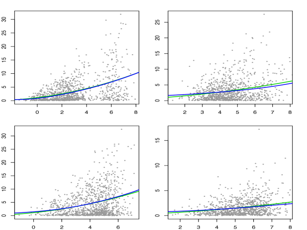
Figure S.7: Results for the variance functions $s^{2}(X)$ produced by the univariate density deconvolution method for each component of ${\mathbf{X}}$ for the conditionally heteroscedastic error distribution $f_{\mbox{\boldmath$\epsilon$}}^{(2)}$ with sample size $n=1000$, $m_{i}=3$ replicates for each subject and component specific covariance matrices with autoregressive structure (AR). The results correspond to the data set that produced the median of the estimated integrated squared errors (ISE) out of a total of 100 simulated data sets for the MIW (mixtures with inverse Wishart priors) method. For each component of ${\mathbf{X}}$, the true variance function is $s^{2}(X)=(1+X/4)^{2}$. See Section 2.2.2 and Section S.3 for additional details. In each panel, the true (lighter shaded green lines) and the estimated (darker shaded blue lines) variance functions are superimposed over a plot of subject specific sample means vs subject specific sample variances. The figure is in color in the electronic version of this article.

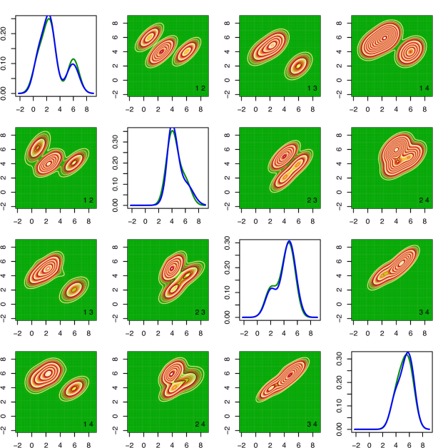
Figure S.8: Results for the $f_{{\mathbf{X}}}$ produced by the MIW (mixtures with inverse Wishart priors) method for the conditionally heteroscedastic error distribution $f_{\mbox{\boldmath$\epsilon$}}^{(2)}$ with sample size $n=1000$, $m_{i}=3$ replicates for each subject and component specific covariance matrices with autoregressive structure (AR). The results correspond to the data set that produced the median of the estimated integrated squared errors (ISE) out of a total of 100 simulated data sets. See Section 6 for additional details. The upper triangular panels show the contour plots of the true two dimensional marginal densities. The lower triangular diagonally opposite panels show the corresponding estimates. The numbers $i,j$ at the bottom right corners of the off-diagonal panels show that the marginal densities $f_{X_{i},X_{j}}$ are plotted in those panels. The diagonal panels show the true (lighter shaded green lines) and the estimated (darker shaded blue lines) one dimensional marginals. The figure is in color in the electronic version of this article.

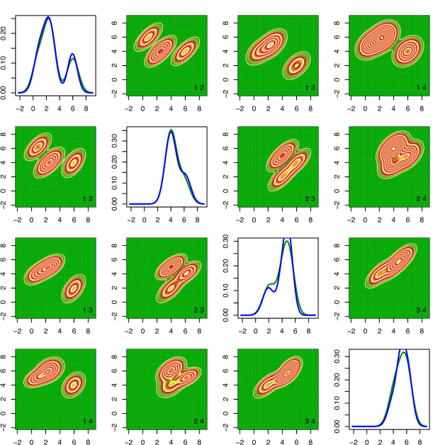
Figure S.9: Results for the $f_{{\mathbf{X}}}$ produced by the MLFA (mixtures of latent factor analyzers) method for the conditionally heteroscedastic error distribution $f_{\mbox{\boldmath$\epsilon$}}^{(2)}$ with sample size $n=1000$, $m_{i}=3$ replicates for each subject and component specific covariance matrices with autoregressive structure (AR). The results correspond to the data set that produced the median of the estimated integrated squared errors (ISE) out of a total of 100 simulated data sets. See Section 6 for additional details. The upper triangular panels show the contour plots of the true two dimensional marginal densities. The lower triangular diagonally opposite panels show the corresponding estimates. The numbers $i,j$ at the bottom right corners of the off-diagonal panels show that the marginal densities $f_{X_{i},X_{j}}$ are plotted in those panels. The diagonal panels show the true (lighter shaded green lines) and the estimated (darker shaded blue lines) one dimensional marginals. The figure is in color in the electronic version of this article.

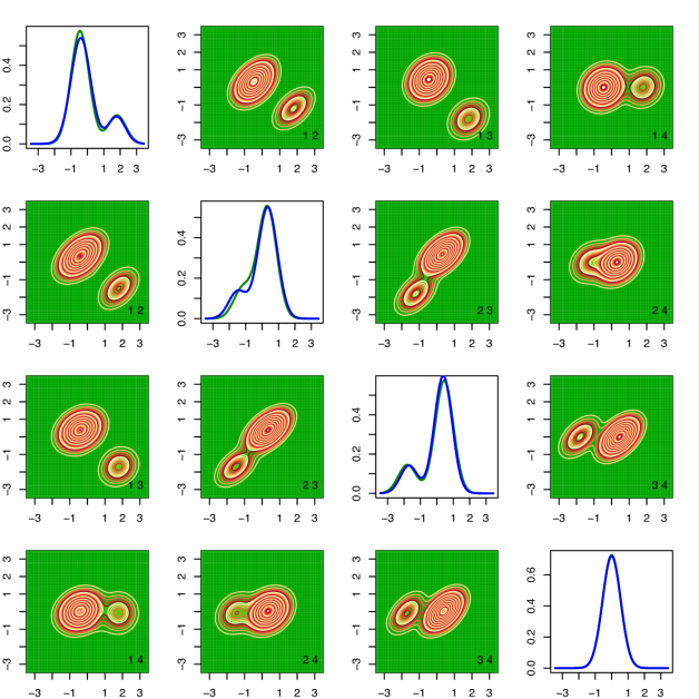
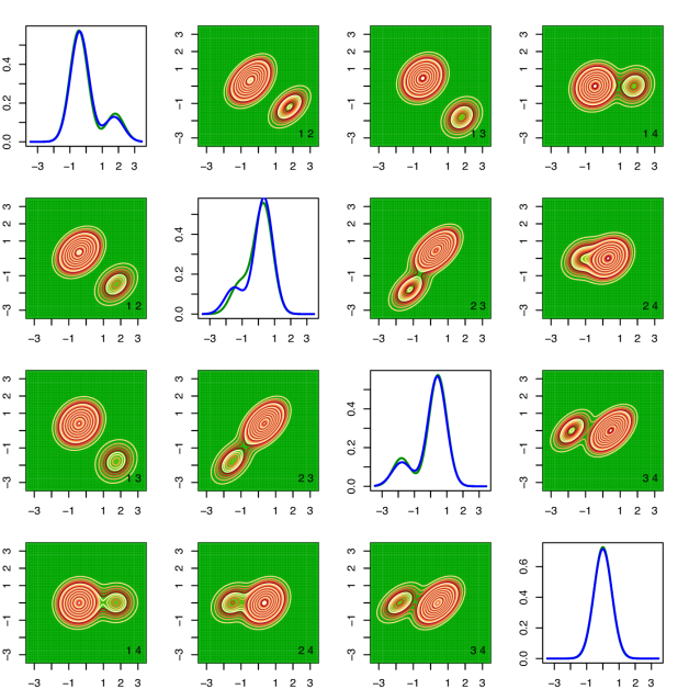
Figure S.10: Results for the density of the scaled errors $f_{\mbox{\boldmath$\epsilon$}}$ produced by the MIW (mixtures with inverse Wishart priors) method for the conditionally heteroscedastic error distribution $f_{\mbox{\boldmath$\epsilon$}}^{(2)}$ with sample size $n=1000$, $m_{i}=3$ replicates for each subject and component specific covariance matrices with autoregressive structure (AR). The results correspond to the data set that produced the median of the estimated integrated squared errors (ISE) out of a total of 100 simulated data sets. See Section 6 for additional details. The upper triangular panels show the contour plots of the true two dimensional marginal densities. The lower triangular diagonally opposite panels show the corresponding estimates. The numbers $i,j$ at the bottom right corners of the off-diagonal panels show that the marginal densities $f_{\epsilon_{i},\epsilon_{j}}$ are plotted in those panels. The diagonal panels show the true (lighter shaded green lines) and the estimated (darker shaded blue lines) one dimensional marginals. The figure is in color in the electronic version of this article.

Figure S.11: Results for the density of the scaled errors $f_{\mbox{\boldmath$\epsilon$}}$ produced by the MLFA (mixtures of latent factor analyzers) method for the conditionally heteroscedastic error distribution $f_{\mbox{\boldmath$\epsilon$}}^{(2)}$ with sample size $n=1000$, $m_{i}=3$ replicates for each subject and component specific covariance matrices with autoregressive structure (AR). The results correspond to the data set that produced the median of the estimated integrated squared errors (ISE) out of a total of 100 simulated data sets. See Section 6 for additional details. The upper triangular panels show the contour plots of the true two dimensional marginal densities. The lower triangular diagonally opposite panels show the corresponding estimates. The numbers $i,j$ at the bottom right corners of the off-diagonal panels show that the marginal densities $f_{\epsilon_{i},\epsilon_{j}}$ are plotted in those panels. The diagonal panels show the true (lighter shaded green lines) and the estimated (darker shaded blue lines) one dimensional marginals. The figure is in color in the electronic version of this article.

Figure S.12: Trace plots and frequency distributions of the number of nonempty clusters produced by the MIW (mixtures with inverse Wishart priors) method for the conditionally heteroscedastic error distribution $f_{\mbox{\boldmath$\epsilon$}}^{(2)}$ with sample size $n=1000$, $m_{i}=3$ replicates for each subject and component specific covariance matrices with autoregressive structure (AR). See Section 6 for additional details. The results correspond to the simulation instance that produced the median of the estimated integrated squared errors (ISE) out of a total of 100 simulated data sets, when the number of mixture components for both $f_{{\mathbf{X}}}$ and $f_{\mbox{\boldmath$\epsilon$}}$ were kept fixed at $K_{{\mathbf{X}}}=6$ and $K_{\mbox{\boldmath$\epsilon$}}=5$. The upper panels are for the $f_{{\mathbf{X}}}$ and the lower panels are for the density of the scaled errors $f_{\mbox{\boldmath$\epsilon$}}$. The true number of mixture components were $K_{{\mathbf{X}}}=3$ and $K_{\mbox{\boldmath$\epsilon$}}=3$. As can be seen from Figure S.10, a mixture model with $2$ nonempty clusters can approximate the true density of the scaled errors well.

Figure S.13: Trace plots and frequency distributions of the number of nonempty clusters produced by the MLFA (mixtures of latent factor analyzers) method for the conditionally heteroscedastic error distribution $f_{\mbox{\boldmath$\epsilon$}}^{(2)}$ with sample size $n=1000$, $m_{i}=3$ replicates for each subject and component specific covariance matrices with autoregressive structure (AR). See Section 6 for additional details. The results correspond to the simulation instance that produced the median of the estimated integrated squared errors (ISE) out of a total of 100 simulated data sets, when the number of mixture components for $f_{{\mathbf{X}}}$ and $f_{\mbox{\boldmath$\epsilon$}}$ were kept fixed at $K_{{\mathbf{X}}}=6$ and $K_{\mbox{\boldmath$\epsilon$}}=5$. The upper panels are for the $f_{{\mathbf{X}}}$ and the lower panels are for the density of the scaled errors $f_{\mbox{\boldmath$\epsilon$}}$. The true number of mixture components were $K_{{\mathbf{X}}}=3$ and $K_{\mbox{\boldmath$\epsilon$}}=3$. As can be seen from Figure S.11, a mixture model with $2$ nonempty clusters can approximate the true density of the scaled errors well.

S.8.3 Additional Figures Summarizing the Results for the EATS Data Set Analyzed in Section 7 of the Main Paper

Figure S.14: Trace plots and frequency distributions of the number of nonempty clusters produced by the MIW (mixtures with inverse Wishart priors) method for the EATS data example. See Section 7 for additional details. The number of mixture components for both $f_{{\mathbf{X}}}$ and $f_{\mbox{\boldmath$\epsilon$}}$ were kept fixed at $K_{{\mathbf{X}}}=K_{\mbox{\boldmath$\epsilon$}}=7$. The upper panels are for the $f_{{\mathbf{X}}}$ and the lower panels are for the density of the scaled errors $f_{\mbox{\boldmath$\epsilon$}}$.

Figure S.15: Trace plots and frequency distributions of the number of nonempty clusters produced by the MLFA (mixtures of latent factor analyzers) method for the EATS data example. See Section 7 for additional details. The number of mixture components for both $f_{{\mathbf{X}}}$ and $f_{\mbox{\boldmath$\epsilon$}}$ were kept fixed at $K_{{\mathbf{X}}}=K_{\mbox{\boldmath$\epsilon$}}=7$. The upper panels are for the $f_{{\mathbf{X}}}$ and the lower panels are for the density of the scaled errors $f_{\mbox{\boldmath$\epsilon$}}$.

S.9 Additional Simulation Experiments

This section presents the results of additional simulation experiments for multivariate t and multivariate Laplace distributed measurement errors. Cases when $f_{{\mathbf{X}}}$ is multivariate t or mixture of multivariate t are also considered. For easy reference, brief descriptions of these distributions are provided below.

S.9.1 Multivariate t Distribution

A random variable $Z$ following a Student’s t-distribution with degrees of freedom $\nu$, mean $\mu$ and variance $\nu b/(\nu-2)$ can be represented as $Z=\mu+\nu^{1/2}b^{1/2}X/Y^{1/2}$, where $Y$ and $X$ are independent, $Y$ follows a chi-square distribution with $\nu$ degrees of freedom, denoted by $Y\sim\chi^{2}_{\nu}$, and $X$ follows a standard normal distribution. A natural extension to multivariate set up is given by ${\mathbf{Z}}=\mbox{\boldmath$\mu$}+\nu^{1/2}\mbox{\boldmath$\Sigma$}^{1/2}{\mathbf{X}}/Y^{1/2}$, where $Y\sim\chi^{2}_{\nu}$ and ${\mathbf{X}}\sim\hbox{MVN}_{p}({\mathbf{0}},{\mathbf{I}})$ independently. The random vector ${\mathbf{Z}}$ is then said to follow a multivariate t-distribution (Kotz and Nadarajah, 2004) with degrees of freedom $\nu$, mean $\mu$ and covariance $\nu\mbox{\boldmath$\Sigma$}/(\nu-2)$, denoted by $\hbox{MVT}_{p}(\nu,\mbox{\boldmath$\mu$},\mbox{\boldmath$\Sigma$})$. The above characterization can be used to sample from a $\hbox{MVT}_{p}(\nu,\mbox{\boldmath$\mu$},\mbox{\boldmath$\Sigma$})$ density. The density of ${\mathbf{Z}}$ is given by

$$f_{{\mathbf{Z}}}({\mathbf{z}})=\frac{\Gamma{\{(\nu+p)/2\}}}{\Gamma{(\nu/2)}(\nu\pi)^{p/2}\left|\mbox{\boldmath$\Sigma$}\right|^{1/2}}\cdot{\{1+({\mathbf{z}}-\mbox{\boldmath$\mu$})^{\rm T}\mbox{\boldmath$\Sigma$}^{-1}({\mathbf{z}}-\mbox{\boldmath$\mu$})/\nu\}^{-(\nu+p)/2}}.$$

The characteristic function is given by

$$\phi({\mathbf{t}})=\exp(i{\mathbf{t}}^{\rm T}\mbox{\boldmath$\mu$})\cdot\frac{||\nu^{1/2}\mbox{\boldmath$\Sigma$}^{1/2}{\mathbf{t}}||^{\nu/2}}{2^{\nu/2-1}\Gamma(\nu/2)}\cdot H_{\nu/2}(||\nu^{1/2}\mbox{\boldmath$\Sigma$}^{1/2}{\mathbf{t}}||),~{}~{}~{}{\mathbf{t}}\in\mathbb{R}^{p},$$

where $H_{\alpha}$ denotes a McDonald’s function of order $\alpha(>1/2)$ and admits the integral representation

$$H_{\alpha}(t)=(2/t)^{\alpha}\cdot\frac{\Gamma(\alpha+1/2)}{\pi^{1/2}}\int_{0}^{\infty}(1+u^{2})cos(tu)du,~{}~{}~{}t>0.$$

When $\mbox{\boldmath$\Sigma$}={\mathbf{I}}$, the identity matrix, the components $Z_{i}$ and $Z_{j}$ are uncorrelated, but not statistically independent. With $\mbox{\boldmath$\mu$}=(\mu_{1}\dots,\mu_{p})^{\rm T}$ and $\mbox{\boldmath$\Sigma$}=((\sigma_{ij}))$, the $i^{th}$ random variable $Z_{i}$ marginally follows a univariate Student’s t-distribution with degrees of freedom $\nu$, mean $\mu_{i}$ and variance $\nu\sigma_{ii}/(\nu-2)$.

S.9.2 Multivariate Laplace Distribution

A random variable $Z$ following a Laplace distribution with mean $\mu$ and variance $b$ has the density

$$f_{Z}(z)=(2b)^{-1/2}\exp(-2^{1/2}b^{-1/2}\left|z-\mu\right|).$$

$Z$ can be represented as $Z=\mu+Y^{1/2}b^{1/2}X$, where $Y$ and $X$ are independent and follow standard exponential and standard normal distributions, respectively. A natural extension to multivariate set up is given by ${\mathbf{Z}}=\mbox{\boldmath$\mu$}+Y^{1/2}\mbox{\boldmath$\Sigma$}^{1/2}{\mathbf{X}}$, where $Y$ follows a standard exponential density and ${\mathbf{X}}\sim\hbox{MVN}_{p}({\mathbf{0}},{\mathbf{I}})$ independently of $Y$. The random vector ${\mathbf{Z}}$ is then said to follow a multivariate Laplace distribution (Eltoft, et al. 2006) with mean $\mu$ and covariance $\Sigma$, denoted by $\hbox{MVL}_{p}(\mbox{\boldmath$\mu$},\mbox{\boldmath$\Sigma$})$. The above characterization can be used to sample from a $\hbox{MVL}_{p}(\mbox{\boldmath$\mu$},\mbox{\boldmath$\Sigma$})$ density. The density of ${\mathbf{Z}}$ is then given by

$$f_{{\mathbf{Z}}}({\mathbf{z}})=\frac{2}{(2\pi)^{p/2}\left|\mbox{\boldmath$\Sigma$}\right|^{1/2}}\cdot\frac{K_{p/2-1}\{2^{1/2}h^{1/2}({\mathbf{z}})\}}{\{h({\mathbf{z}})/2\}^{p/4-1/2}},$$

where $h({\mathbf{z}})=({\mathbf{z}}-\mbox{\boldmath$\mu$})^{\rm T}\mbox{\boldmath$\Sigma$}^{-1}({\mathbf{z}}-\mbox{\boldmath$\mu$})$ and $K_{m}$ denotes modified Bessel functions of the second kind of order $m$. Using asymptotic formula for the Bessel functions, namely $K_{m}(z)=\{\pi/(2z)\}^{1/2}\exp(-z)$ as $\left|z\right|\to\infty$, we have

$$f_{{\mathbf{Z}}}({\mathbf{z}})\approx\frac{\pi^{1/2}}{(2\pi)^{p/2}\left|\mbox{\boldmath$\Sigma$}\right|^{1/2}}\cdot\frac{2^{(p-1)/4}}{h^{(p-1)/4}({\mathbf{z}})}\cdot\exp\{-2^{1/2}h^{1/2}({\mathbf{z}})\}.$$

The characteristic function is given by $\phi({\mathbf{t}})=\exp(i{\mathbf{t}}^{\rm T}\mbox{\boldmath$\mu$})(1+{\mathbf{t}}^{\rm T}\mbox{\boldmath$\Sigma$}{\mathbf{t}}/2)^{-1}$ for ${\mathbf{t}}\in\mathbb{R}^{p}$. For $p>1$, the density has a singularity at $\mu$. When $\mbox{\boldmath$\Sigma$}={\mathbf{I}}$, the identity matrix, the components $Z_{i}$ and $Z_{j}$ are uncorrelated, but not statistically independent. With $\mbox{\boldmath$\mu$}=(\mu_{1}\dots,\mu_{p})^{\rm T}$ and $\mbox{\boldmath$\Sigma$}=((\sigma_{ij}))$, the $i^{th}$ random variable $Z_{i}$ marginally follows a univariate Laplace distribution with mean $\mu_{i}$ and variance $\sigma_{ii}$.

S.9.3 Summary of Results

The results of the simulation experiments the measurement errors are distributed according to $f_{\mbox{\boldmath$\epsilon$}}^{(3)}=\hbox{MVT}_{4}(6,{\mathbf{0}},\mbox{\boldmath$\Sigma$})$ and $f_{\mbox{\boldmath$\epsilon$}}^{(4)}=\hbox{MVL}_{4}({\mathbf{0}},\mbox{\boldmath$\Sigma$})$ probability laws independently of ${\mathbf{X}}$ are presented in Table S.1. The results for conditionally heteroscedastic measurement errors are presented in Table S.2. In both cases, ${\mathbf{X}}$ is distributed according to the mixture of multivariate normals described in Section 6 of the main paper. As in the main paper, in each case four different choices for the covariance matrix $\Sigma$ were considered. The general patterns of the estimated MISEs are similar to that observed in Table 2 of the main paper where the true measurement error distributions were finite mixtures of multivariate normal kernels. While in theory the MLFA model described in the main paper can approximate distributions like the multivariate Laplace that puts significant mass around the origin, in practice, since it assumes $\mbox{\boldmath$\Omega$}_{k}=\mbox{\boldmath$\Omega$}=\hbox{diag}\{\sigma_{1}^{2},\dots,\sigma_{p}^{2}\}$ for all $k$, it often smooths out the spikes at the origin. A mild variation, referred to as the $\text{MLFA}_{2}$ model, that instead assumes $\mbox{\boldmath$\Omega$}_{k}=\sigma_{k}^{2}\hbox{I}_{p}$ and results in slight improvement in the MISE performance is also included in Table S.1 and Table S.2. For the simulation experiments and the real data analysis presented in the main text, the two versions of the MLFA model perform very similarly and the latter version was not included. Results for conditionally heteroscedastic multivariate Laplace errors with diagonal covariance structure are summarized in Figures S.16-S.22 with observations similar to those discussed in Section 6 of the main paper.

True Error Distribution	Covariance Structure	Sample Size	MISE $\times 10^{4}$
			$\text{MLFA}_{2}$	MLFA	MIW	Naive
(c) Multivariate t	I	500	1.06	1.38	3.98	12.32
		1000	0.53	0.65	1.54	9.91
	LF	500	6.62	8.26	7.57	47.22
		1000	4.73	5.78	3.65	45.70
	AR	500	12.69	13.56	6.14	40.76
		1000	11.36	9.16	3.45	39.59
	EXP	500	7.84	8.42	5.00	26.85
		1000	6.26	6.64	2.38	26.04
(d) Multivariate Laplace	I	500	1.08	1.32	3.08	8.22
		1000	0.50	0.63	1.20	6.25
	LF	500	4.41	5.57	5.66	32.31
		1000	2.38	3.53	2.84	31.10
	AR	500	8.38	8.72	5.14	27.30
		1000	6.08	6.19	2.56	26.19
	EXP	500	5.24	5.67	4.14	17.57
		1000	3.58	4.17	1.98	16.86

Table S.1: Mean integrated squared error (MISE) performance of MLFA (mixtures of latent factor analyzers) and MIW (mixtures with inverse Wishart priors) density deconvolution models for homoscedastic errors compared with a naive method that ignores measurement errors for different measurement error distributions. See Section 2 and Section S.9 for additional details. The minimum value in each row is highlighted.

True Error Distribution	Covariance Structure	Sample Size	MISE $\times 10^{4}$
			$\text{MLFA}_{2}$	MLFA	MIW	Naive
(c) Multivariate t	I	500	2.78	3.25	24.48	19.10
		1000	1.39	1.53	13.40	17.75
	LF	500	12.65	14.72	52.77	69.64
		1000	6.71	8.43	25.66	66.49
	AR	500	20.54	23.2	43.22	64.07
		1000	13.53	18.41	21.42	59.81
	EXP	500	11.56	14.12	37.68	43.57
		1000	8.19	11.97	18.22	41.66
(d) Multivariate Laplace	I	500	1.81	2.32	9.60	10.31
		1000	0.97	1.20	4.20	8.86
	LF	500	7.33	10.30	17.52	41.89
		1000	3.99	5.28	7.65	40.93
	AR	500	9.79	14.13	15.64	35.50
		1000	5.54	9.32	6.59	34.91
	EXP	500	7.26	9.90	13.93	23.71
		1000	3.90	5.12	5.19	22.78

Table S.2: Mean integrated squared error (MISE) performance of MLFA (mixtures of latent factor analyzers) and MIW (mixtures with inverse Wishart priors) density deconvolution models for conditionally heteroscedastic errors compared with a naive method that ignores measurement errors for different measurement error distributions. See Section 2 and Section S.9 for additional details. The minimum value in each row is highlighted.

We also extend the simulation experiments to scenarios when ${\mathbf{X}}$ is distributed according to (B) $f_{{\mathbf{X}}}^{(3)}=\hbox{MVT}_{4}(6,\mbox{\boldmath$\mu$}_{{\mathbf{X}}},\mbox{\boldmath$\Sigma$}_{{\mathbf{X}}}),\mbox{\boldmath$\mu$}_{{\mathbf{X}}}=(2,2,2,2)^{\rm T}$, (C) $f_{{\mathbf{X}}}^{(4)}=\sum_{k=1}^{2}\pi_{{\mathbf{X}},k}\hbox{MVT}_{4}(6,\mbox{\boldmath$\mu$}_{{\mathbf{X}},k},\mbox{\boldmath$\Sigma$}_{{\mathbf{X}}})$, $\mbox{\boldmath$\pi$}_{{\mathbf{X}}}=(0.75,0.25)^{\rm T},\mbox{\boldmath$\mu$}_{{\mathbf{X}},1}=(2,4,2,2)^{\rm T},\mbox{\boldmath$\mu$}_{{\mathbf{X}},2}=(4,2,4,2)^{\rm T}$. In each case, four different choices for $\mbox{\boldmath$\Sigma$}_{{\mathbf{X}}}$ are considered as in Section 6 of the main paper. We focus on the case when the measurement errors are conditionally heteroscedastic. Results are presented in Tables S.3 and S.4.

True Distribution of Interest $f_{{\mathbf{X}}}$	True Error Distribution $f_{\mbox{\boldmath$\epsilon$}}$	Covariance Structure	Sample Size	MISE $\times 10^{4}$
				$\text{MLFA}_{2}$	MIW	Naive
(B) Multivariate t	(a) Multivariate Normal	I	500	4.35	20.36	18.17
			1000	2.36	13.14	12.65
		LF	500	21.31	78.22	75.42
			1000	15.57	52.73	67.77
		AR	500	33.18	59.77	63.33
			1000	29.29	51.11	53.40
		EXP	500	19.58	40.72	44.83
			1000	17.78	32.01	37.58
	(b) Mixture of Multivariate Normals	I	500	5.16	27.21	38.03
			1000	2.87	18.17	35.99
		LF	500	27.89	73.75	159.29
			1000	19.27	53.66	161.77
		AR	500	38.41	81.77	159.34
			1000	34.22	55.25	156.05
		EXP	500	21.95	45.76	100.33
			1000	18.14	37.72	99.09
	(c) Multivariate t	I	500	4.16	27.73	23.42
			1000	2.34	19.87	20.36
		LF	500	22.83	91.04	90.39
			1000	14.03	85.33	89.31
		AR	500	40.60	76.40	86.87
			1000	36.93	70.76	75.19
		EXP	500	26.36	55.65	61.25
			1000	18.51	40.46	49.52
	(d) Multivariate Laplace	I	500	3.93	16.48	16.14
			1000	1.81	6.85	14.02
		LF	500	16.36	47.19	70.22
			1000	12.13	27.64	59.48
		AR	500	29.46	42.44	63.79
			1000	18.81	21.19	47.92
		EXP	500	19.00	34.74	39.64
			1000	13.30	16.24	32.76

Table S.3: Mean integrated squared error (MISE) performance of MLFA (mixtures of latent factor analyzers) and MIW (mixtures with inverse Wishart priors) density deconvolution models for conditionally heteroscedastic errors compared with a naive method that ignores measurement errors for different measurement error distributions. See Section 2 and Section S.9 for additional details. The minimum value in each row is highlighted.

True Distribution of Interest $f_{{\mathbf{X}}}$	True Error Distribution $f_{\mbox{\boldmath$\epsilon$}}$	Covariance Structure	Sample Size	MISE $\times 10^{4}$
				$\text{MLFA}_{2}$	MIW	Naive
(C) Mixture of Multivariate t	(a) Multivariate Normal	I	500	4.84	13.68	12.43
			1000	2.82	7.41	10.15
		LF	500	21.62	30.01	47.95
			1000	13.40	19.72	44.97
		AR	500	22.56	29.35	43.99
			1000	19.80	25.59	39.63
		EXP	500	18.36	27.27	28.00
			1000	13.41	17.73	25.14
	(b) Mixture of Multivariate Normals	I	500	5.39	14.64	22.90
			1000	2.80	10.77	21.55
		LF	500	24.48	32.87	98.00
			1000	15.62	20.52	98.79
		AR	500	26.73	31.09	90.78
			1000	23.44	29.06	91.24
		EXP	500	19.56	25.39	58.83
			1000	13.90	18.29	59.93
	(c) Multivariate t	I	500	4.91	18.09	16.30
			1000	2.89	11.59	14.00
		LF	500	23.50	33.79	60.18
			1000	15.85	25.83	58.20
		AR	500	26.98	33.78	54.07
			1000	22.04	29.77	51.64
		EXP	500	18.62	24.00	36.26
			1000	12.64	18.57	33.61
	(d) Multivariate Laplace	I	500	4.76	9.34	15.96
			1000	2.33	5.04	13.96
		LF	500	16.59	22.54	65.33
			1000	11.69	13.41	59.25
		AR	500	24.73	26.21	58.87
			1000	15.71	17.48	47.62
		EXP	500	14.26	19.12	34.53
			1000	10.96	13.25	32.47

Table S.4: Mean integrated squared error (MISE) performance of MLFA (mixtures of latent factor analyzers) and MIW (mixtures with inverse Wishart priors) density deconvolution models for conditionally heteroscedastic errors compared with a naive method that ignores measurement errors for different measurement error distributions. See Section 2 and Section S.9 for additional details. The minimum value in each row is highlighted.

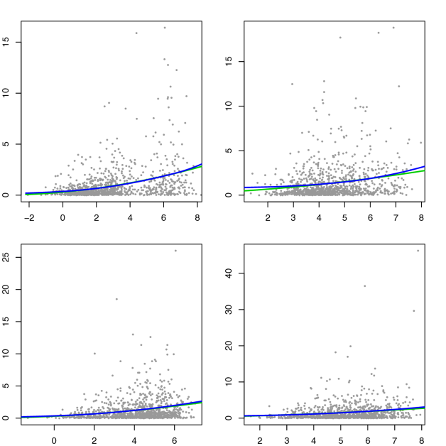
Figure S.16: Results for the variance functions $s^{2}(X)$ produced by the univariate density deconvolution method for each component of ${\mathbf{X}}$ for conditionally heteroscedastic multivariate Laplace ($f_{\mbox{\boldmath$\epsilon$}}^{(4)}$) distributed measurement errors with sample size $n=1000$, $m_{i}=3$ replicates for each subject and identity matrix (I) for the component specific covariance matrices. The results correspond to the data set that produced the median of the estimated integrated squared errors (ISE) out of a total of 100 simulated data sets for the MIW (mixtures with inverse Wishart priors) method. For each component of ${\mathbf{X}}$, the true variance function is $s^{2}(X)=(1+X/4)^{2}$. See Section 2.2.2 and Section S.3 for additional details. In each panel, the true (lighter shaded green lines) and the estimated (darker shaded blue lines) variance functions are superimposed over a plot of subject specific sample means vs subject specific sample variances. The figure is in color in the electronic version of this article.

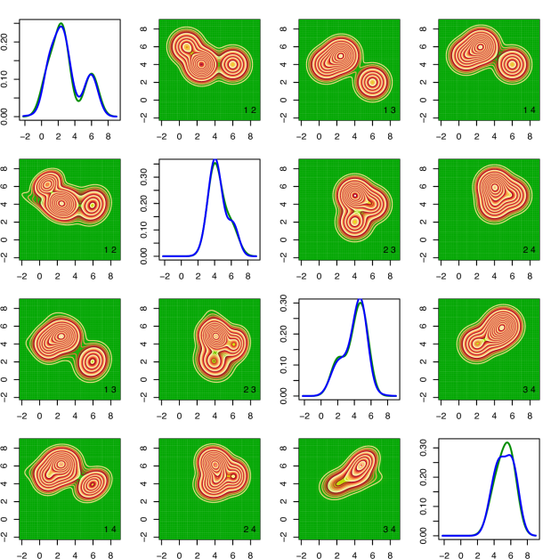
Figure S.17: Results for the $f_{{\mathbf{X}}}$ produced by the MIW (mixtures with inverse Wishart priors) method for conditionally heteroscedastic multivariate Laplace ($f_{\mbox{\boldmath$\epsilon$}}^{(4)}$) distributed measurement errors with sample size $n=1000$, $m_{i}=3$ replicates for each subject and identity matrix (I) for the component specific covariance matrices. The results correspond to the data set that produced the median of the estimated integrated squared errors (ISE) out of a total of 100 simulated data sets. See Section 6 and Section S.9 for additional details. The upper triangular panels show the contour plots of the true two dimensional marginal densities. The lower triangular diagonally opposite panels show the corresponding estimates. The numbers $i,j$ at the bottom right corners of the off-diagonal panels show that the marginal densities $f_{X_{i},X_{j}}$ are plotted in those panels. The diagonal panels show the true (lighter shaded green lines) and the estimated (darker shaded blue lines) one dimensional marginals. The figure is in color in the electronic version of this article.

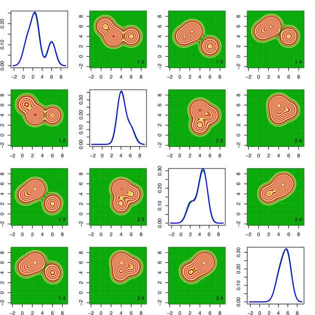
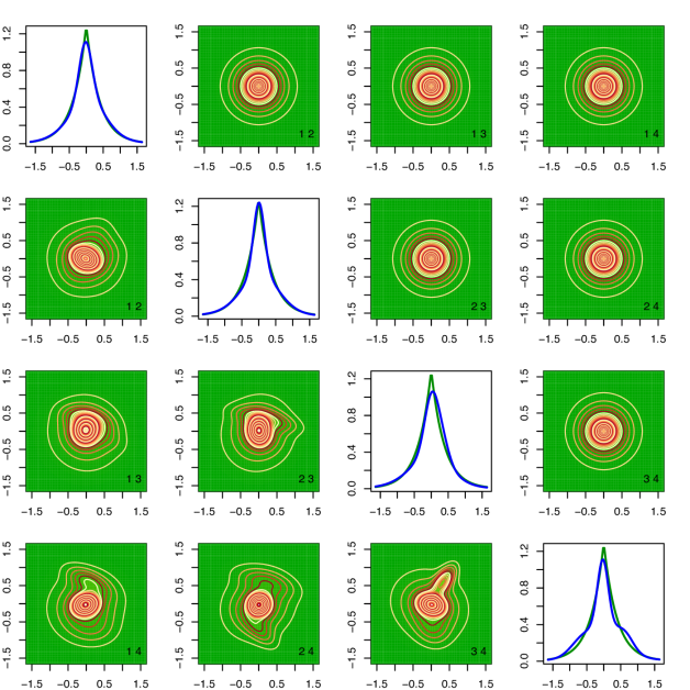
Figure S.18: Results for the $f_{{\mathbf{X}}}$ produced by the $\text{MLFA}_{2}$ (mixtures of latent factor analyzers) method for conditionally heteroscedastic multivariate Laplace ($f_{\mbox{\boldmath$\epsilon$}}^{(4)}$) distributed measurement errors with sample size $n=1000$, $m_{i}=3$ replicates for each subject and identity matrix (I) for the component specific covariance matrices. The results correspond to the data set that produced the median of the estimated integrated squared errors (ISE) out of a total of 100 simulated data sets. See Section 6 and Section S.9 for additional details. The upper triangular panels show the contour plots of the true two dimensional marginal densities. The lower triangular diagonally opposite panels show the corresponding estimates. The numbers $i,j$ at the bottom right corners of the off-diagonal panels show that the marginal densities $f_{X_{i},X_{j}}$ are plotted in those panels. The diagonal panels show the true (lighter shaded green lines) and the estimated (darker shaded blue lines) one dimensional marginals. The figure is in color in the electronic version of this article.

Figure S.19: Results for the density of the scaled errors $f_{\mbox{\boldmath$\epsilon$}}$ produced by the MIW (mixtures with inverse Wishart priors) method for conditionally heteroscedastic multivariate Laplace ($f_{\mbox{\boldmath$\epsilon$}}^{(4)}$) distributed measurement errors with sample size $n=1000$, $m_{i}=3$ replicates for each subject and identity matrix (I) for the component specific covariance matrices. The results correspond to the data set that produced the median of the estimated integrated squared errors (ISE) out of a total of 100 simulated data sets. See Section 6 and Section S.9 for additional details. The upper triangular panels show the contour plots of the true two dimensional marginal densities. The lower triangular diagonally opposite panels show the corresponding estimates. The numbers $i,j$ at the bottom right corners of the off-diagonal panels show that the marginal densities $f_{\epsilon_{i},\epsilon_{j}}$ are plotted in those panels. The diagonal panels show the true (lighter shaded green lines) and the estimated (darker shaded blue lines) one dimensional marginals. The figure is in color in the electronic version of this article.

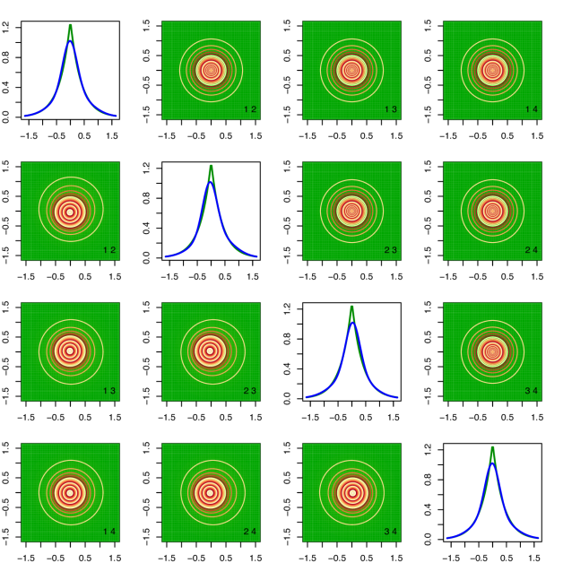
Figure S.20: Results for the density of the scaled errors $f_{\mbox{\boldmath$\epsilon$}}$ produced by the $\text{MLFA}_{2}$ (mixtures of latent factor analyzers) method for conditionally heteroscedastic multivariate Laplace ($f_{\mbox{\boldmath$\epsilon$}}^{(4)}$) distributed measurement errors with sample size $n=1000$, $m_{i}=3$ replicates for each subject and identity matrix (I) for the component specific covariance matrices. The results correspond to the data set that produced the median of the estimated integrated squared errors (ISE) out of a total of 100 simulated data sets. See Section 6 and Section S.9 for additional details. The upper triangular panels show the contour plots of the true two dimensional marginal densities. The lower triangular diagonally opposite panels show the corresponding estimates. The numbers $i,j$ at the bottom right corners of the off-diagonal panels show that the marginal densities $f_{\epsilon_{i},\epsilon_{j}}$ are plotted in those panels. The diagonal panels show the true (lighter shaded green lines) and the estimated (darker shaded blue lines) one dimensional marginals. The figure is in color in the electronic version of this article.

Figure S.21: Trace plots and frequency distributions of the number of nonempty clusters produced by the MIW (mixtures with inverse Wishart priors) method for conditionally heteroscedastic multivariate Laplace ($f_{\mbox{\boldmath$\epsilon$}}^{(4)}$) distributed measurement errors with sample size $n=1000$, $m_{i}=3$ replicates for each subject and identity matrix (I) for the component specific covariance matrices. See Section 6 and Section S.9 for additional details. The upper panels are for the $f_{{\mathbf{X}}}$ and the lower panels are for the density of the scaled errors $f_{\mbox{\boldmath$\epsilon$}}$. The results correspond to the simulation instance that produced the median of the estimated integrated squared errors (ISE) out of a total of 100 simulated data sets, when the number of mixture components for both $f_{{\mathbf{X}}}$ and $f_{\mbox{\boldmath$\epsilon$}}$ were kept fixed at $K_{{\mathbf{X}}}=5$ and $K_{\mbox{\boldmath$\epsilon$}}=6$, respectively.

Figure S.22: Trace plots and frequency distributions of the number of nonempty clusters produced by the $\text{MLFA}_{2}$ (mixtures of latent factor analyzers) method for conditionally heteroscedastic multivariate Laplace ($f_{\mbox{\boldmath$\epsilon$}}^{(4)}$) distributed measurement errors with sample size $n=1000$, $m_{i}=3$ replicates for each subject and identity matrix (I) for the component specific covariance matrices. See Section 6 and Section S.9 for additional details. The upper panels are for the $f_{{\mathbf{X}}}$ and the lower panels are for the density of the scaled errors $f_{\mbox{\boldmath$\epsilon$}}$. The results correspond to the simulation instance that produced the median of the estimated integrated squared errors (ISE) out of a total of 100 simulated data sets, when the number of mixture components for $f_{{\mathbf{X}}}$ and $f_{\mbox{\boldmath$\epsilon$}}$ were kept fixed at $K_{{\mathbf{X}}}=7$ and $K_{\mbox{\boldmath$\epsilon$}}=5$, respectively.

S.10 Potential Impact on Nutritional Epidemiology

The joint distribution of long-term average intakes of different dietary components allows nutritionists to study the dietary habits of the population of interest in fine detail. The plots of pairwise marginal distributions presented in Figure 8, for instance, provide detailed information on the joint consumption patterns of different pairs of dietary components. While such graphical summaries of the joint distributions may not be available for more than two components, numerical summaries of the joint distribution can provide answers to important questions such as what proportion of the population consume certain dietary components above, between or below certain amounts etc. The last question is particularly important as it relates to the proportion of the population that are deficient in certain dietary components. Focusing again on a two-dimensional case for illustration, namely Fiber and Potassium, Figure S.23 below shows their marginal and joint cumulative distribution function (CDF) on a set of grid points from which such proportions can be readily obtained. Dietary components are often reported in different measurement units. The figures presented in Section 7 are based on a linear scale transformation $W_{ij\ell}=20\times\{W_{ij\ell,obs}-W_{ij\ell,obs,min}\}/\{W_{ij\ell,obs,max}-W_{ij\ell,obs,min}\}$ so that the $W_{ij\ell}$ for different components are unitless and fall between 0 and 20 units. Figure S.23 report the marginal and the joint CDF of fiber and potassium on a set of grid points in their original measurement units. We can readily see that, considered jointly, approximately $59\%$ of adult Americans consume less than 20.55 grams of fiber and 3338.55 milligrams of potassium, whereas the corresponding marginal values are $71.2\%$ and $67.6\%$, respectively.

The focus of the nutritional epidemiology examples considered in this article were on the estimation of joint consumption patterns of a set of regularly consumed dietary components whose reported intakes were all continuously measured. In contrast, for dietary components that are consumed episodically, the reported intakes equal zero on non-consumption days, and are positive on consumption days. The methodology developed in this article paves the way to more sophisticated deconvolution methods that can accommodate such zero inflated data. We are pursuing this problem as the subject of a separate study, with promising preliminary results. This will be a crucial step forward towards providing a highly flexible statistical framework for estimating the distribution of the U.S. Department of Agriculture’s Healthy Eating Index (HEI, www.cnpp.usda.gov/HealthyEatingIndex.htm). HEI is a measure of diet quality that involves six episodically and seven regularly consumed dietary components and is used to assess compliance with the U.S. Dietary Guidelines for Americans (www.health.gov/dietaryguidelines) and monitor changes in dietary patterns. Efficient estimation of the distribution of HEI will allow nutritionists to answer public health questions that have important policy implications. We expect successful implementation of our methods to eventually replace the currently popular NCI method (www.riskfactor.cancer.gov/diet/usualintakes/method.html) for estimation of HEI.

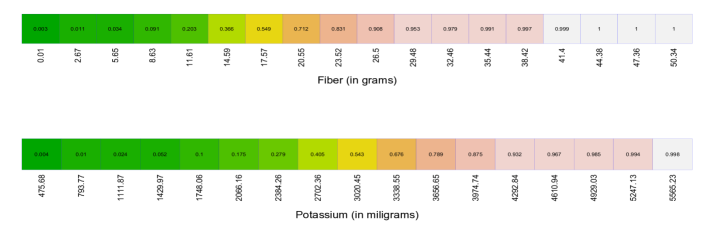
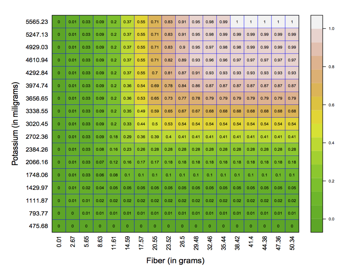
Figure S.23: Results for Fiber and Potassium in their commonly used measurement units. The top two panels show their marginal cumulative distribution functions. The bottom panel shows their joint cumulative distribution function for a set of grid points. The figure is in color in the electronic version of this article.

Additional References

Bickel, P. J. and Kleijn, B. J. K. (2012). The semiparametric Bernstein-von Mises theorem. Annals of Statistics, 40, 206-237.

Bontemps, D. (2011). Bernstein-von Mises theorems for Gaussian regression with increasing number of regressors. Annals of Statistics, 39, 2557-2584.

Carroll, R. J., Chen X. and Hu, Y. (2010). Identification and estimation of nonlinear models using two samples with nonclassical measurement errors. Journal of Nonparametric Statistics, 22, 379-399.

Castillo, I. and Nickl, R. (2014). On the Bernstein-von Mises phenomenon for nonparametric Bayes procedures. Annals of Statistics, 42, 1941-1969.

de Boor, C. (2000). A Practical Guide to Splines. New York: Springer.

d’Haultfoeuille, X. (2011). On the completeness condition in nonparametric instrumental problems. Econometric Theory, 27, 460-471.

Eltoft, T., Kim, T. and Lee, T. W. (2006). On the multivariate Laplace distribution. IEEE Signal Processing Letters, 13, 300-303.

Escobar, M. D. and West, M. (1995). Bayesian density estimation and inference using mixtures. Journal of the American Statistical Association, 90, 577-588.

Eubank, R. L. and Hart, J. D. (1992). Testing goodness-of-fit in regression via order selection criteria. Annals of Statistics, 20, 1412-1425.

Ferguson, T. F. (1973). A Bayesian analysis of some nonparametric problems. Annals of Statistics, 1, 209-230.

Fraley, C. and Raftery, A. E. (2007). Model-based methods of classification: using the mclust software in chemometrics. Journal of Statistical Software, 18, 1-13.

Ghosh, J. K. and Ramamoorthi, R. V. (2010). Bayesian Nonparametrics. New York: Springer.

Goldberg, R. R . (1961). Fourier transforms. Volume 32. London: Cambridge.

Green, J. P., Latuszynski, K. Pereyra, M. and Roberts, C. P. (2015). Bayesian computation: summary of the current state, and samples backwards and forwards. Statistics and Computing, 25, 835-862.

Hastie, D. I., Liverani, S. and Richrdson, S. (2015). Sampling from Dirichlet process mixture models with unknown concentration parameter: mixing issues in large data implementations. Statistics and Computing, 25, 1023-1037.

Ishwaran, H. and James, L. F. (2002). Approximate Dirichlet process computing in finite normal mixtures: smoothing and prior information. Journal of Computational and Graphical Statistics, 11, 508-532.

Ishwaran, H. and Zarepour, M. (2000). Markov chain Monte Carlo in approximate Dirichlet and beta two-parameter process hierarchical models. Biometrika, 87, 371-390.

Ishwaran, H. and Zarepour, M. (2002). Exact and approximate sum-representations for the Dirichlet process. Canadian Journal of Statistics, 30, 269-283.

Johnstone, I. M. (2010). High dimensional Bernstein-von Mises: simple examples. Institute of Mathematical Statistics Collections, 6, 87-98.

Kotz, S. and Nadarajah, S. (2004). Multivariate t Distributions and Their Applications. Cambridge: Cambridge University Press.

Neal, R. M. (2000). Markov chain sampling methods for Dirichlet process mixture models. Journal of Computational and Graphical Statistics, 9, 249-265.

Norets, A. and Pelenis, J. (2012). Bayesian modeling of joint and conditional distributions. Journal of Econometrics, 168, 332-346.

Pati, D. and Dunson, D. (2013). Bayesian nonparametric regression with varying residual density. Annals of the Institute of Statistical Mathematics, 66, 1-13.

Pelenis, J. (2014). Bayesian Regression with Heteroscedastic Error Density and Parametric Mean Function. Journal of Econometrics, 178, 624-638.

Rocke, D. and Durbin, B. (2001). A model for measurement error for gene expression arrays. Journal of Computational Biology, 8, 557-569.

Rousseau, J. and Mengersen, K. (2011). Asymptotic behavior of the posterior distribution in overfitted mixture models Journal of the Royal Statistical Society, Series B, 73, 689-710.

Sethuraman, J. (1994). A constructive definition of Dirichlet priors. Statistica Sinica, 4, 639-650.

Spokoiny, V. (2013). Bernstein-von Mises theorem for growing parameter dimension. arXiv preprint arXiv:1302.3430.