Counterexamples to Cantorian Set Theory

Abstract

This paper provides some counterexamples to Cantor’s contributions to the foundations of Set Theory. The paper starts with a very basic counterexample to Cantor’s Diagonal Method (DM) applied to binary fractional numbers that forces it to yield one of the numbers in the target list. To study if this specific case is just an anomaly or rather a deeper source for concern, and given that for the DM to work the list of numbers have to be written down, the set of numbers that can be represented using positional fractional notation, $\mathbb{W}$, is properly characterized. It is then shown that $\mathbb{W}$ is not isomorphic to $\mathbb{R}$, the set of all real numbers. This fact means that results obtained from the application of the DM to $\mathbb{W}$ in order to derive properties of $\mathbb{R}$ are not valid. After showing that $\mathbb{W}$ can be trivially well-ordered, application of the DM to some shuffles of the ordered list of the set of binary numbers $\mathbb{W_{\textrm{2}}}$ is proven to always converge to a number in the list. This result is then used to generate a counterexample to Cantor’s DM for a generic list of reals that forces it to yield one of the numbers of the list, thus invalidating Cantor’s result that infers the non-denumerability of $\mathbb{R}$ from the application of the DM to $\mathbb{W}$. After this apparently anomalous result we are forced to question Cantor’s Theorem about the different cardinalities of a set and its power set, and by means of another counterexample we show that Cantor’s Theorem does not actually hold for infinite sets. After analyzing all these counterexamples, it is shown that the current notion of cardinality for infinite sets does not depend on the "size" of the sets, but rather on the representation chosen for them. Following this line of thought, the concept of model as a framework for the construction of the representation of a set is introduced, and a theorem is proven showing that an infinite set can be well-ordered if there is a proper model for it. To reiterate that the cardinality of a set does not determine whether the set can be well-ordered, a set of cardinality $\aleph_{0}^{\aleph_{0}}=2^{\aleph_{0}}=\mathfrak{c}$ is proven to be equipollent to the set of natural numbers $\mathbb{N}$. The paper concludes with an analysis of the cardinality of the ordinal numbers, for which a representation of cardinality $\aleph_{0}^{\aleph_{0}}$ is proposed.

1 Introduction

The contributions of Georg Cantor to Set Theory [1, 2] have been controversial since their very inception. Perhaps his most shocking and counterintuitive result is the apparent existence of different types of infinity. His Diagonal Argument to show the different cardinalities of the natural and real numbers is particularly noteworthy, and has pervaded other areas of mathematics such as Logic and Computability theory.

In this paper we will see that the cardinality of infinite sets seems to be determined by the representation we choose for them, rather than by their "size". We will also demonstrate that Cantor’s Diagonal Method (DM) can be forced to produce one of the listed numbers under some conditions.

Since attacking such a controversial yet widely accepted theory will surely face some strong opposition, the paper is mostly structured around counterexamples that are easy to explain and verify. The paper follows the research path the author, which should make it more approachable to general readers. Those familiar with Cantorian Set Theory may want to skip directly to Section 7.

In this paper we will start with a minimalistic counterexample to the DM and analyze it to see where it leads. We will find that the DM works not on the set of reals $\mathbb{R}$, but on the set of writable numbers $\mathbb{W}$. The fact that these sets are not isomorphic is the source of the DM’s apparently paradoxical consequences. In particular it will be proved that for some orderings of the set $\mathbb{W_{\textrm{2}}}$ of numbers writable in base 2 the DM always yields a number on the list. Using this result and the fact that the DM needs to enter $\mathbb{W}_{b}$ for some base b will permit us to show in section 7 that there are shufflings of the list of all numbers in $\mathbb{R}$ that force the DM to yield one of the numbers of the list. This result effectively invalidates the most widely accepted proof of the non-denumerability of the real numbers.

This erratic behavior of Cantor’s DM leads us to questioning the validity of Cantor’s Theorem, which states that a set and its power-set always have different cardinality. While this is obviously true for finite sets, Cantor relied on the DM to demonstrate its validity for infinite sets; and after seeing the counterexamples for $\mathbb{W_{\textrm{2}}}$ and $\mathbb{W_{\textrm{10}}}$ for the special case of the non-denumerability of the reals we are forced to examine his general result in more detail. Ultimately we are able to provide a specific counterexample to Cantor’s Theorem by producing a bijection between the set of non-negative integers and its power-set in section 8.

In section 8.1 we introduce the Applicative Numbering model to sort a set of size $\aleph_{0}^{\aleph_{0}}=2^{\aleph_{0}}=\mathfrak{c}$. This proves that cardinality by itself is not a limiting factor for whether a set can be well-ordered or not. In fact, we see in section 9 that there are very specific conditions that a representation of a set must verify for it to be well-orderable. The most important conclusion of the paper is that the standard positional numbering model (section 9.2) does not meet one of the conditions, which is the main reason why the DM has been incorrectly taken to imply that $\mathbb{R}$ is non-denumerable.

To conclude, the paper presents some tentative models for the real and the ordinal numbers, and implications to the Continuum Hypothesis are discussed.

2 A minimalistic counterexample to Cantor’s Diagonal Method

Cantor claims that for every infinite list of reals in $[0,1)$, all of them different, it is possible to find a number not contained in the list by application of his Diagonal Method (see for instance [3] for a basic introduction). Table 1 presents one simple counterexample using a list $L_{1}$ of binary fractional numbers. The third column shows the antidiagonal number $\bar{D}$ resulting from the Diagonal Method (DM) applied to $L_{1}$ up to digit n, where the notation $\text{\"{\i}\textquestiondown\oe}|_{k}$ is used to denote truncation of the string of digits up to digit k. The fourth column shows where in the list $L_{1}$ can the partial result $\bar{D}\left(L_{1}\right)|_{n}$ be found.

Table 1: A list $L_{1}(n)$ of fractional binary numbers and the partial results of the antidiagonal number $\bar{D}$ up to digit n. Fourth and fifth columns show every partial antidiagonal result is already in the list.

We can see that: (1) any partial result of the DM, $\bar{D}\left(L_{1}\right)|_{k}$, is equal to the next number on the list $L_{1}(k+1)$, and (2) the limiting antidiagonal number $\bar{D}$ is equivalent to the very first number on the list.

There is nevertheless a difference in form between the antidiagonal number and the first number of the list: one uses 1-ending representation and the other 0-ending. This fact was known to Cantor and Dedekind (see [4], p.191) and it’s usually overlooked as an irrelevant inconvenience to Cantor’s arguments. Yet, if we are going to be perfectly strict, we need to completely understand if this is a cause for concern or not, and why.

For now let’s just agree that the binary strings 0.10000… and 0.01111… both represent the same real number $1/2$. After this rather trivial observation, Table 1 seems to suggest that the DM doesn’t work as expected for at least one list $L_{1}$. And that happens neither (1) after any finite number of steps, nor (2) after extrapolation to the limiting result (that is, after an infinity of steps).

Note that in Table 1 there are no dots after the partial results, since these are finite strings of length k for any number of iterations k. Note as well that these partial strings ensure the current $\bar{D}\left(L_{1}\right)|_{k}$—of length k—is different from any of the strings found on lines 1 to k, that is, up to any finite number of iterations. Cantor’s argument extrapolates these partial results to the case where k grows to infinity, which he envisions should make sure the limiting $\bar{D}\left(L_{1}\right)=\lim_{k\rightarrow\infty}\bar{D}\left(L_{1}\right)|_{k}$ is different from every string in the list, and should therefore correspond to a completely new number not contained in the list.

However, after the admittedly simplistic counterexample shown in Table 1, the generalization of Cantor’s extrapolation to any list of reals doesn’t seem to be as straightforward as it may have first appeared, because, at least in principle, there is nothing preventing every partial antidiagonal result of k digits $\bar{D}\left(L\right)|_{k}$ from being found somewhere ahead of line k in an infinite list L. In the example shown above this happens to occur just on the next line, $k+1$—and for that matter on any lines after k. This shows the list may in fact contain a subsequence that converges to the same limiting number $\bar{D}$. It is not clear then what the purpose of the DM actually is: does it find one of the limits of the list? Does the limit even belong to the same set as the numbers being listed? These are important details that we need to study in order to determine the soundness of Cantor’s Diagonal Method.

Moreover, is the set of reals properly represented when symbolized by a list of character strings written in positional fractional notation? We will see in the next section that this is not the case.

3 The set of all numbers that can be written

The key point to understand where the problems with the DM originate is that real numbers don’t "have" digits. For instance, $\pi$ is defined as the ratio of the length of a circle to its diameter; there are no digits in this, in principle, purely geometrical description. However, it is very convenient to use positional fractional notation in base 10 to say that $\pi$ is about 3.1416, provided we don’t forget that this concatenation of digits is not $\pi$ itself. The fact that the DM targets a list of written numbers means that it is not targeting $\mathbb{R}$ directly, but rather a convenient representation of it, $\mathbb{W}$. This seemingly trivial observation has serious consequences, as we shall see. To begin with, it means we have to be very careful when deriving properties of $\mathbb{R}$ through the analysis of the set of writable numbers $\mathbb{W}$, especially if they happen to be completely different sets. We will study the question within this section.

Most of what follows are well-known elementary math results. However, I haven’t been able to find them collected to specifically characterize the set of writable numbers $\mathbb{W}$, so they are included here for completion.

First of all, we need to define what a writable number is: a number writable in positional fractional notation for some natural base $b>1$ is a finite string of digits smaller than b and with a dot separating the integer and fractional parts of the number:

$$\forall b>1\in\mathbb{N}:w=w_{p}\ldots w_{1}w_{0}.w_{-1}w_{-2}\ldots w_{-q}\in\mathbb{W}_{b}\Leftrightarrow p,q\in\mathbb{Z}^{+}\,\wedge\,0\leq w_{k}<b\in\mathbb{Z}^{+}$$ (1)

A $+$ or $-$ symbol may be placed at the beginning of the string to indicate the sign of the number, but since negative numbers are of no interest for the matter discussed in this paper, we will assume from now on that $\mathbb{W}$ only concerns non-negative numbers.

These writable numbers are just the standard numbers we use every day, with $b=10$ being the most common base (decimal numbers). The numbers in base $b=2$ (binary numbers) are also important, being the most convenient choice for computational applications.

It is easy to show that the set of all numbers that can be written in a given base b, $\mathbb{W}_{b}$, is not isomorphic to the set of real numbers $\mathbb{R}$ because (1) every writable number in $\mathbb{W}_{b}$ has an image in $\mathbb{R}$ (its value), but (2) there are numbers in $\mathbb{R}$ that cannot be written in $\mathbb{W}_{b}$.

The real value x of a writable number w in $\mathbb{W}_{b}$ can be obtained by summation of the products of its digits to the powers of b according to the position of the digits in the string:

$$\textrm{Val}:\mathbb{W}_{b}\to\mathbb{R}$$ (2)

$$w=w_{p}\ldots w_{1}w_{0}.w_{-1}w_{-2}\ldots w_{-q}\in\mathbb{W}_{b}$$ (3)

$$x=\textrm{Val}\left(w\right)\equiv\sum\nolimits_{k=-q}^{p}{w_{k}\cdot b^{k}}\in\mathbb{R}$$ (4)

The real number x and its fractional positional number notation w are different things indeed, but this is easy to forget given our routine use of $\mathbb{W}_{10}$ to speak about numbers in $\mathbb{R}$. For instance, given that the string $w="123.5"$ and its corresponding real value $x=\mathrm{Val}\left("123.5"\right)=1\cdot 100+2\cdot 10+3+5/10=123.5$ happen to be the same written string may make us unconsciously identify w with x, and therefore $\mathbb{W}_{10}$ with $\mathbb{R}$ for any number. Yet, the number x in $\mathbb{R}$ described by 123.5 in decimal can also be written down as 1111011.1 in binary; x is neither of those strings. These seemingly trivial comments will be very relevant when we realize that some of Cantor’s derivations suffer from an implicit association of $\mathbb{W}$ with $\mathbb{R}$. This association breaks down when we consider numbers with an infinite tail of digits, with the exception of the trivial terminations …000… and …(b-1) (b-1) (b-1)…, which do have equivalent writable representations within $\mathbb{W}_{b}$.

It is easy to show that $\mathbb{W}_{b}$ is in fact a subset of $\mathbb{Q}$, the set of rational numbers. The proof is a well known result:

$$\forall w=w_{p}\ldots w_{1}w_{0}.w_{-1}\ldots w_{-q}\in\mathbb{W}_{b}:\exists z\in\mathbb{Z},\exists n\in\mathbb{N}|\mathrm{Val}\left(w\right)=\frac{z}{n}\in\mathbb{Q}$$ (5)

$$Proof:\>\mathrm{Val}\left(w\right)=\sum\limits_{k=-q}^{p}{w_{k}\cdot b^{k}}=\frac{\sum\nolimits_{k=-q}^{p}{w_{k}\cdot b^{q+k}}}{b^{q}}=\frac{z}{n}\in\mathbb{Q}$$

To show that $\mathbb{W}_{b}$ is a proper subset of $\mathbb{Q}$ we just need to prove that some numbers in $\mathbb{Q}$ (and therefore in $\mathbb{R}$) cannot be represented with a finite number of digits:

$$\forall b>1\in\mathbb{N}\>\exists x\in\mathbb{Q}\>|\>\nexists w\in\mathbb{W}_{b}:\mathrm{Val}\left(w\right)=x$$ (6)

$$Proof:\>Take\thinspace x=\frac{1}{p}\in\mathbb{Q}\thinspace with\thinspace p\thinspace prime\thinspace and\thinspace p>b$$

$$Assume\thinspace\exists w\in\mathbb{W}_{b}\>|\>x=\mathrm{Val}\left(w\right)=\mathrm{Val}(0.w_{1}w_{2}\ldots w_{n})\thinspace with\thinspace n\in\mathbb{N}\Rightarrow$$

$$\Rightarrow\frac{1}{p}=\frac{w_{1}b^{n-1}+w_{2}b^{n-2}+\cdots+w_{n}}{b^{n}}\Rightarrow$$

$$\Rightarrow\frac{b^{n}}{p}=w_{1}b^{n-1}+w_{2}b^{n-2}+\cdots+w_{n}\in\mathbb{N}\Rightarrow p\thinspace divides\thinspace b\thinspace(contradiction)$$

Therefore $\mathbb{W}_{b}$ is a proper subset of $\mathbb{Q}$ and thus of $\mathbb{R}$:

$$\mathrm{Val}\left(\mathbb{W}_{b}\right)\subset\mathbb{Q}\subset\mathbb{R}$$ (7)

However, the closure of $\mathbb{W}_{b}$ for any b is the set of all real numbers written in that base $\mathbb{R}_{b}$:

$$\forall b>1\in\mathbb{N}:\mathrm{Cl}\left(\mathbb{W}_{b}\right)=\mathbb{R}_{b}$$ (8)

And therefore the value of the closure is the set of all real numbers $\mathbb{R}$:

$$\forall b>1\in\mathbb{N}:\mathrm{Val}\left(\mathrm{Cl}\left(\mathbb{W}_{b}\right)\right)=\mathrm{Val}\left(\mathbb{R}_{b}\right)=\mathbb{R}$$ (9)

We can prove 9 by showing that any real number can be approximated to any level of precision using a written positional expansion:

$$\forall x\in\mathbb{R\>}\forall\varepsilon>0\in\mathbb{R\>}\exists w\in\mathbb{W}_{b}\,|\,\left\|x-\mathrm{Val}(w)\right\|<\varepsilon$$ (10)

$$Proof:\thinspace\forall\varepsilon>0\>\exists k\in\mathbb{Z}^{+}|-k<\log_{b}\varepsilon\Rightarrow b^{-k}<\varepsilon$$

$$w=x|_{k}=x_{p}\ldots x_{1}x_{0}.x_{-1}x_{-2}\ldots x_{-k}\in\mathbb{W}_{b}\Rightarrow$$

$$\Rightarrow\left\|x-\mathrm{Val}(w)\right\|=0.00\ldots 00x_{-k-1}x_{-k-2}\ldots<0.00\ldots 01=b^{-k}<\varepsilon$$

To complete the characterization of $\mathbb{W}_{b}$, and because it will be of use in following sections, it is interesting to note that the set can be expressed as the internal direct sum of the subset of numbers with null fractional part $\mathbb{W}_{b}^{I}$ and the subset of numbers with null integer part $\mathbb{W}_{b}^{F}$:

$$\mathbb{W}_{b}=\mathbb{W}_{b}^{I}\oplus\mathbb{W}_{b}^{F}$$ (11)

$$\mathbb{W}_{b}^{I}\equiv\left\{w=w_{p}\ldots w_{1}w_{0}.w_{-1}w_{-2}\ldots w_{-q}\in\mathbb{W}_{b}\,|\,\mathrm{Val}\left(0.w_{-1}\ldots w_{-q}\right)=0\right\}$$ (12)

$$\mathbb{W}_{b}^{F}\equiv\left\{w=w_{p}\ldots w_{1}w_{0}.w_{-1}w_{-2}\ldots w_{-q}\in\mathbb{W}_{b}\,|\,\mathrm{Val}\left(w_{p}\ldots w_{1}w_{0}.0\right)=0\right\}$$ (13)

Which is straightforward since every element w in $\mathbb{W}_{b}$ can be expressed as the sum of one element from $\mathbb{W}_{b}^{I}$ (its integral part) and another from $\mathbb{W}_{b}^{F}$ (its fractional part):

$$w=w_{p}\ldots w_{1}w_{0}.w_{-1}w_{-2}\ldots w_{-q}=w_{p}\ldots w_{1}w_{0}+0.w_{-1}w_{-2}\ldots w_{-q}=\left\lfloor w\right\rfloor+\left\{w\right\}$$ (14)

It is easy to see that the set of values of the elements in $\mathbb{W}_{b}^{I}$ is $\mathbb{Z}^{+}$, so we could write that $\mathbb{W}_{b}^{I}$ is just the representation of $\mathbb{Z}^{+}$ in base b, $\mathbb{Z}_{b}^{+}$:

$$\mathbb{W}_{b}^{I}=\mathrm{Base}{}_{b}\left(\mathbb{Z}^{+}\right)\equiv\mathbb{Z}_{b}^{+}$$ (15)

$$\mathbb{Z}^{+}=\mathrm{Val}\left(\mathbb{W}_{b}^{I}\right)$$ (16)

On the other hand $\mathbb{W}_{b}^{F}$ is the set of fractional real numbers in [0, 1) which can be written down using finitely many significant digits. We can denote this interval as $\left[0,1\right)_{\mathbb{W}_{b}}$ to distinguish it from the representation in base b of the fractional reals $\left[0,1\right)_{b}$, which contains numbers with infinitely many significant digits:

$$\mathbb{W}_{b}^{F}=[0,\thinspace 1)\cap\mathbb{W}_{b}\equiv[0,\thinspace 1)_{\mathbb{W}_{b}}$$ (17)

$$\mathrm{Val}\left([0,\thinspace 1)_{\mathbb{W}_{b}}\right)\subset\mathrm{Val}\left([0,\thinspace 1)_{b}\right)=[0,\thinspace 1)\subset\mathbb{R}$$ (18)

Therefore, using (11), $\mathbb{W}_{b}$ can be seen as the Cartesian product of the set of integers in base b with the set of those fractional numbers in [0, 1) that can actually be written down. This means $\mathbb{W}_{b}$ is missing some elements present in the positional fractional representation of $\mathbb{R}$ in base b, $\mathbb{R}_{b}$:

$$\mathbb{W}_{b}=\mathbb{Z}_{b}^{+}\times[0,\thinspace 1)_{\mathbb{W}_{b}}\subset\mathbb{Z}_{b}^{+}\times[0,\thinspace 1)_{b}=\mathbb{R}_{b}^{+}$$ (19)

There is nothing really new on the results shown so far in this section: it is well known that some real numbers require a never-ending expansion of digits when written in fractional positional notation. Some of these are irrational or transcendental, but many others are just rationals. Nevertheless, it was important to characterize $\mathbb{W}$ properly in order to show more interesting results in following sections.

The differences between $\mathbb{W}$ and $\mathbb{R}$ directly mean that it is impossible to write a list of all real numbers using positional fractional notation, since some numbers just can’t be written with finitely many digits. Cantor could have stopped there, but instead moved further ahead, applying the DM to a list of written numbers without realizing he wasn’t targeting $\mathbb{R}$, but a different set, $\mathbb{W}$. He concludes then that there are “more” numbers in $\mathbb{R}$ than those on any list of writable numbers (which in a way is true, as we have seen). But from there (or, more precisely, after he determined the cardinality of $\mathbb{R}$ to be $2^{\aleph_{0}}$ plus the application of the DM to support Cantor’s Theorem) he incorrectly infers that the reason had to be that $\mathbb{R}$ is "unlistable" (non-denumerable). We will see in more detail why this inference is not justified in the following sections of the paper and provide some supporting counterexamples.

Regarding the previous paragraph, an important remark must be made: some readers may argue that by considering tails of infinitely many digits we can in fact target $\mathbb{R}$ instead of $\mathbb{W}$; unfortunately this is irrelevant, because the DM only considers digits at finite positions, so those numbers with infinite tails are completely indistinguishable to the DM from numbers in $\mathbb{W}$. Therefore, the only quality that could differentiate those “unwrittable” reals from members of $\mathbb{W}$ is not used at all by the DM. We will later exploit this weakness of the DM to produce a counterexample that invalidates its application to proving the non-denumerability of $\mathbb{R}$.

We will see in the next section that $\mathbb{W}$ can actually be well-ordered and is therefore denumerable. After that we will apply the DM to one ordered list of $\mathbb{W}$, and find the key result that for $\mathbb{W}_{2}$ the DM can be forced to always yield a number explicitly written in the initial list (this is not always true when using other bases b>2). We will combine this result with the weakness mentioned in the previous paragraph to construct the equivalent counterexample for the list of all real numbers.

4 A well-ordering for all binary writable numbers $\mathbb{W}_{2}$

From now on I will be moving to binary numbers since they produce more compact tables and are enough to prove that the DM cannot be used to justify the non-denumerability of the reals. Most of the results we’ll find can be applied to other bases b>2. Some versions of the DM for b=10 are studied in Section 6.

To well-order $\mathbb{W}_{2}$ we first need to well order is fractional part $\mathbb{W}_{2}^{F}=[0,\thinspace 1)_{\mathbb{W}_{2}}$ by finding a bijection that maps any non-negative integer to a number in $\mathbb{W}_{2}^{F}$ and vice versa. Fortunately this is not difficult to do: just revert the order of the digits of every binary non-negative integer $n=x_{1}x_{2}\ldots x_{k}$ to create a fractional number between zero and one. This Digital Inversion (DI) process operates as follows:

$$\mathrm{DI}\thinspace:\thinspace\mathbb{Z}^{+}\to[0,\thinspace 1)_{\mathbb{W}_{2}}\subset\mathbb{W}_{2}\subset\mathbb{R}$$ (20)

$$n=x_{1}x_{2}\ldots x_{k}\in\mathbb{Z}^{+},\thinspace x_{i}\in\{0,\thinspace 1\}$$ (21)

$$\mathrm{DI}\left(n\right)=\mathrm{DI}\left(x_{1}x_{2}\ldots x_{k}\right)\equiv 0.x_{k}\ldots x_{2}x_{1}\in[0,\thinspace 1)_{\mathbb{W}_{2}}$$ (22)

An algorithm that applies the DI function to an enumeration of the set of non-negative integers $\mathbb{Z}^{+}$ using base 2 results in the list $L_{\mathrm{DI}}$ shown in Table 2.

Table 2: The list $L_{\mathrm{DI}}$ of all possible fractional numbers that can be written in base 2.

Note that for fractional numbers with finitely many significant digits the DI function is invertible, and can therefore be used to find the position in the list of the fractional number:

$$\mathrm{Pos}\left(x=0.x_{1}x_{2}\ldots x_{k}\right)=\mathrm{DI}^{-1}\left(0.x_{1}x_{2}\ldots x_{k}\right)=x_{k}\ldots x_{2}x_{1}=\thinspace n\in\mathbb{Z}^{+}$$ (23)

The function DI therefore establishes a bijection between $\mathbb{Z}^{+}$ and $\left[0,1\right)_{\mathbb{W}_{2}}$ which suffices to produce a well-ordering of $\left[0,1\right)_{\mathbb{W}_{2}}$.

If a fractional number has infinitely many significant digits the DI function can still be used to find the position in $L_{\mathrm{DI}}$ of every approximation up to any digit k:

$$\mathrm{DI}^{-1}\left(0.x_{1}x_{2}x_{3}\ldots|_{k}\right)=x_{k}\ldots x_{2}x_{1}=\thinspace n\in\mathbb{Z}^{+}$$ (24)

Note that the way $L_{\mathrm{DI}}$ is constructed trivially guarantees that every block of $2^{n}$ consecutive lines contains all possible fractional numbers that can be written using any combination of n digits. This by the way implies that any partial fractional number $0.x_{1}x_{2}\ldots x_{k}$ can be found not only at position $n=x_{k}\ldots x_{2}x_{1}$ but also at infinitely many positions $1x_{k}\ldots x_{2}x_{1}$, $10x_{k}\ldots x_{2}x_{1}$, $11x_{k}\ldots x_{2}x_{1}$, $100x_{k}\ldots x_{2}x_{1}$, … ahead of line n in $L_{\mathrm{DI}}$.

Note also that every possible real number x in the closed interval [0, 1] is either in $L_{\mathrm{DI}}$ or is a limit of it. The proof is essentially the same used to show that $\mathrm{Cl}\left(\mathbb{W}_{b}\right)=\mathbb{R}$ in the previous section 10.

Moving on, we just showed that $\left[0,1\right)_{\mathbb{W}_{2}}$ is denumerable, and we saw before that $\mathbb{W}_{2}$ is equivalent to the Cartesian product of $\mathbb{Z}_{2}^{+}$ and $\left[0,1\right)_{\mathbb{W}_{2}}$. Therefore, a list of all binary writable numbers can be composed using Cantor’s procedure for enumerating the rational numbers. In this way we can create a 2D matrix listing on one axis the set of non-negative integers and on the other the ordered set of all writable fractional expansions $L_{\mathrm{DI}}$as shown in Table 3.

Table 3: The Cartesian product of the integer and fractional parts of $\mathbb{W}_{2}$.

We then traverse it diagonally to obtain a sorted list of all binary writable numbers in $\mathbb{W}_{2}$:

$$L\left(\mathbb{W}_{2}\right)=\left\{0.0,\thinspace 0.1,\thinspace 1.0,\thinspace 0.01,\thinspace 1.1,\thinspace 10.0,\thinspace 0.11,\thinspace 1.01,\thinspace 10.1,\thinspace 11.0,\thinspace 0.001,\thinspace 1.11,\thinspace 10.01,\thinspace 11.1,\thinspace 100.0,\thinspace\ldots\right\}$$ (25)

Since $L\left(\mathbb{W}_{2}\right)$ is just an ordering of the elements of $\mathbb{W}_{2}$, the closure of $L\left(\mathbb{W}_{2}\right)$ is the set of all real binary numbers $\mathbb{R}_{2}$, as we saw in section 3:

$$\mathrm{Cl}\left(L\left(\mathbb{W}_{2}\right)\right)=\mathrm{Cl}\left(\mathbb{W}_{2}\right)=\mathbb{R}_{2}$$ (26)

These results can be easily generalized to any other base different than 2, meaning that all $\mathbb{W}_{b}$ can be well-ordered and are therefore denumerable.

Note however that the closure of $\mathbb{W}_{b}$ cannot be well-ordered in the same lexicographic fashion as $\mathbb{W}_{b}$ is, since infinitely many elements of the closure require infinitely many significant digits and therefore correspond to the same limiting "position" of infinity (this is what Cantor actually found, but that the reals are not denumerable does not follow from this fact, as we shall see in section 9.2). Nevertheless, some numbers in the closure’s boundary are equivalent in $\mathbb{R}$ (that is, have the same value) to members of $\mathbb{W}_{b}$, namely all those that end in an infinite tail of repeated 0 digits or of repeated (b-1) digits. This will be essential to demonstrate that the DM fails in general to provide a non-listed number in base 2, as presented in the next section.

I’ll be using the notation $L\left(S\right)$ throughout the paper to denote a listing of a given set S, as done above without introduction. This will imply that S admits a well-ordering, that is, can be put into one-to-one correspondence with the set of non-negative integers. We may then write $L_{\mathrm{DI}}=L\left([0,\thinspace 1)_{\mathbb{W}_{2}};\,\mathrm{DI}\right)$ where the element after the semicolon indicates the mapping function. We can make the well-ordering property for a set S explicit by writing $\exists L\left(S\right)$.

5 Application of the DM to $L_{\mathrm{DI}}$

Direct application of the DM to $L_{\mathrm{DI}}$ results in the limiting number $\overline{D}=0.11111\ldots$ which doesn’t belong to [0, 1) nor is explicitly written on the list, even if every partial expansion $0.11111\ldots|{}_{\mathrm{k}}$ is. A simple way to make it converge to a number in a finite position of the list is to apply a shuffle $S$ to the rows of $L_{\mathrm{DI}}$, generating a new list $L_{\mathrm{DI}}^{{}^{\prime}}$. Consider this very simple shuffle $S_{0}$:

$$S_{0}\thinspace:\thinspace\mathbb{Z}^{+}\to\mathbb{Z}^{+}$$ (27)

$$S_{0}\left(n\right)=\left\{\begin{array}[]{cc}1-n&if\thinspace n\leq 1\\ n&if\thinspace n>1\end{array}\right.$$ (28)

When applied to $L_{\mathrm{DI}}$, $S_{0}$ swaps the first two rows. Let’s define $L_{\mathrm{DI}}^{{}^{\prime}}\left(n\right)=\left(S_{0}\ast L_{\mathrm{DI}}\right)\left(n\right)=L_{\mathrm{DI}}\left(S_{0}\left(n\right)\right)$ and see what the application of the DM yields for this case; the result is shown in Table 4.

Table 4: A shuffling of the list of all writable numbers in [0, 1) and the result of the application of the DM.

And we see that the value of the limiting antidiagonal number $\bar{D}$ actually matches that of the first number on the list; also, any partial result of the DM can be found somewhere ahead on the list. Here, again, we need to be especially careful in keeping in mind that the strings in $\mathbb{W}_{2}$ and the numbers they represent in $\mathbb{R}$ are different objects. So, it doesn’t matter that $L_{\mathrm{DI}}^{{}^{\prime}}\left(0\right)=0.10000\ldots$ and $\bar{D}\left(L_{\mathrm{DI}}^{{}^{\prime}}\right)=0.01111\ldots$ are different binary strings, because their values in $\mathbb{R}$ are the same: $\mathrm{Val}\left(L_{\mathrm{DI}}^{{}^{\prime}}\left(0\right)\right)=\mathrm{Val}\left(\bar{D}\left(L_{\mathrm{DI}}^{{}^{\prime}}\right)\right)=1/2\in\mathbb{R}$

To make this distinction clear we can think of the DM as a black box that takes a list of reals $L$ and outputs a real number $\bar{D}$ (Figure 1). Inside the box we first have to convert the list of reals to a list of strings in $\mathbb{W}_{b}$ using a base b positional fractional notation; from those strings we obtain the diagonal number $D_{b}$, and from it the antidiagonal number in base b, $\overline{D}_{b}$. Application of the Val function to $\overline{D}_{b}$ yields the final output $\bar{D}\in\mathbb{R}$.

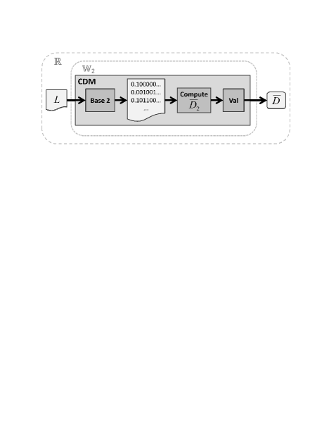
Figure 1: A block diagram representation of Cantor’s Diagonal Method (CDM) using base 2.

So, to summarize what we saw in this section, we started with an infinite list $L_{\mathrm{DI}}^{{}^{\prime}}$ of reals, all of them different, put them through a black box called DM and obtained an output $\bar{D}$ whose value actually matches that of one of the reals in $L_{\mathrm{DI}}^{{}^{\prime}}$. This seems to indicate that Cantor’s Diagonal Argument can’t possibly work in general, since we have found at least one specific case where it fails to produce a number not on the input list. Furthermore, $L_{\mathrm{DI}}^{{}^{\prime}}$ contains every fractional number that can be written, so it is not at all clear how the situation could be more or less favorable for the DM if we consider as well the missing unwritable reals in [0, 1).

It may be that this counterexample is just an anomaly, and that the DM actually works well for the list of all reals $L\left(\mathbb{R}\right)$. But we will see in section 7 that this is not the case: the DM also fails for the list of all reals in [0, 1). Before that, however, we need to address a minor detail on the implementation of the DM black box.

6 Addressing other variants of Cantor’s Diagonal Method

Some readers may point out that the lists provided so far are "wrong", because we are supposed to make sure the numbers on the list use the 1-ending representation of the real numbers that have the infinite termination …xyz01111… instead of the equivalent 0-ending representation …xyz10000… This requirement appears in many texts discussing the DM (e.g. [5, 6]) and seems to have originated in 1877 when Dedekind pointed it out to Cantor as a potential problem with Cantor’s proof of the equipollence of $\mathbb{R}$ and $\mathbb{R}^{n}$ (see [4], p.191).

If we are to use the 1-ending criterion we may have to discard 0 and target (0, 1) or (0, 1] instead of [0, 1), because 0 doesn’t have an equivalent 1-ending representation. In any case, applying any of these extra conditions doesn’t make any significant difference to the performance of the DM. To prove it let’s create a version of the list without 0.0 in it and using the 1-ending version of the numbers to obtain a new list $L_{\mathrm{DI}}^{{}^{\prime\prime}}$ meeting these more stringent requirements.

The result is presented in Table 5 where it can be seen that the DM also yields a listed number when using the 1-ending representation for the input list. Note that in this case we didn’t even need to add a shuffle function to make it converge to a number explicitly on the list. Here I must again remind the reader that the strings in $L_{\mathrm{DI}}^{{}^{\prime\prime}}$ and $\bar{D}$ are in positional notation and we still need to apply the Val function (4) to obtain the actual numbers they represent in $\mathbb{R}$. In this way we observe $\mathrm{Val}\left(L_{\mathrm{DI}}^{{}^{\prime\prime}}\left(3\right)\right)=\mathrm{Val}\left(\bar{D}\left(L_{\mathrm{DI}}^{{}^{\prime\prime}}\right)\right)=3/4\in\mathbb{R}$.

Table 5: A binary representation of the list of all writable numbers in [0, 1) using 1-ending termination and the result of the application of Cantor’s Diagonal Method.

Other flavors of the DM concern the number base used. In base 10, which is the variant most commonly used in popular math books, you can prevent the antidiagonal number from converging to an explicit number on the list by choosing the replacement digits properly. Table 6 summarizes the results for some implementations of the DM in base 10 found in math vulgarization books when applied to $L_{\mathrm{DI}}$. The most commonly found version is the one that adds 1 to every digit modulo 10, and can be found in Stephen Hawking’s "God Created the Integers" [6] and many others [3, 7]; this version can be forced to fail, and the same happens with D. R. Hofstadter’s variation [8] that subtracts 1 from every digit modulo 10. On the other hand, R. Penrose’s version [9] cannot be forced to yield a number on the list, and the resulting antidiagonal number is an unwritable rational. W. Dunham’s approach [10] uses random digits, which can neither be forced to fail (but note that random numbers cannot be generated by a purely mathematical process—they require an entropy source, which is a physical device).

Table 6: Results of the application of the DM to $L_{\mathrm{DI}}$ in base 10 for some of the variants found in popular math vulgarization books.

With regard to the replacement digit criterion, the base 2 case for the DM is especially hopeless. Given that in base 2 there are only two available symbols it is always possible to find a shuffling of the list that forces a never-ending …111… or …000… trivial termination for the antidiagonal number, which as we have seen converges to numbers in the closure of $\mathbb{W}_{2}$ that are also representable within $\mathbb{W}_{2}$. This situation can ultimately be forced because the positional fractional notation is more efficient at producing strings (numbers) than the DM is at discarding them. Considering that $L_{\mathrm{DI}}$ only needs $\log_{2}\left(n\right)$ digits to represent the number at line n and the DM needs to swap digit n to clear the number at line n, this implies the DM will eventually find an area where there are no longer any significant digits (meaning the trivial …111… and …000… infinite terminations on the list). Consequently, the DM will—for infinitely many appropriate shuffling functions of $L_{\mathrm{DI}}$, if needed—end in a constant tail of 1s or 0s (depending on the flavor chosen for the DM), thus converging into a number that can be represented by a finite number of digits and will therefore be explicitly contained within $L_{\mathrm{DI}}$.

7 Application of the DM to a generic list of reals

What if instead of applying the DM to $L\left([0,\thinspace 1)_{\mathbb{W}_{2}}\right)$ we used $L\left([0,\thinspace 1)\right)$ as an input? Would the DM produce a noticeably different result? That could perhaps indicate that the DM can tell apart lists of denumerable sets and list of (presumably) non-denumerable sets–although it is very unlikely because the DM black box (Figure 1) requires first to write down the numbers using positional notation, and there are no more written numbers than those in $L\left(\mathbb{W}\right)$.

In this section we will just demonstrate that some orderings of $L\left(\mathbb{R}\right)$ also force the DM to yield an antidiagonal number $\overline{D}$ that is already in $L\left(\mathbb{R}\right)$. The proof relies in the previously mentioned fact that the DM cannot distinguish unwritable real numbers (with infinitely many significant digits) from numbers in $\mathbb{W}$, and therefore we can make sure our input list of reals yields one of the numbers of the list by replicating, for instance, the "skeleton" of the list $L_{\mathrm{DI}}^{{}^{\prime\prime}}$ shown in Table 5—which we know forces the DM to fail.

So we start with a list $L_{R}=L\left((0,\thinspace 1]\right)$ which we assume contains all real numbers in (0, 1] written using 1-ending termination and proceed to construct a reordering of it, $L_{R}^{{}^{\prime}}$, in the following way:

1. Start by making $L_{R}^{{}^{\prime}}=L_{R}$.

2. Find the number 3/4 (the real value of $0.101111\ldots_{2}$) in $L_{R}^{{}^{\prime}}$ and move it to line 3, shifting the rest of the list as needed.

3. Starting from line 1, check if the k^th binary digit of $L_{R}^{{}^{\prime}}\left(k\right)$ using 1-ending representation matches that of $L_{\mathrm{DI}}^{{}^{\prime\prime}}\left(k\right)$. If it does, do nothing; otherwise look ahead in $L_{R}^{{}^{\prime}}$ until you find an index m such that $L_{R}^{{}^{\prime}}\left(m\right)$ matches the k^th digit, then swap lines m and k in $L_{R}^{{}^{\prime}}$.

4. Repeat step 3 until the whole list has been reordered.

An example of application of this procedure is shown in Table 7.

Table 7: A reordering $L_{R}^{{}^{\prime}}$ of the list $L_{R}$ of the reals in [0,1) so that its diagonal and third element match those of $L_{\mathrm{DI}}^{{}^{\prime\prime}}$.

With this reordering of $L_{R}$ we are sure to obtain $L_{R}^{{}^{\prime}}\left(3\right)$ when applying the binary DM, since $L_{R}^{{}^{\prime}}$ and $L_{\mathrm{DI}}^{{}^{\prime\prime}}$ are indistinguishable to the DM. Figure 2 summarizes what we have achieved.

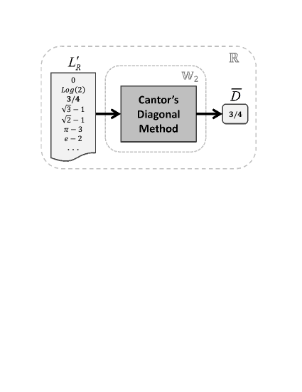
Figure 2: The list $L_{R}^{{}^{\prime}}$ of the reals in [0,1), which has been specially engineered to force Cantor’s Diagonal Method to yield the third element of the list when working on base 2. Note that the DM block must always operate within a proper subset of $\mathbb{R}$, $\mathbb{W}_{b}$.

We can then conclude that there is at least one shuffling of $L_{R}$ that forces the DM to yield a number explicitly listed. Therefore we have just proved that it is not true that for any given list of the reals in (0,1] the DM is always able to produce a number not on the list.

Also, we have shown that the representation of the input list plays an essential role in the outcome of the procedure: in base 2 we can force the DM to fail, but for other bases b>2—and some careful selection of the replacement digits—it can still perform as expected. We will see later that this is not a mere coincidence, and that the cardinality of infinite sets is determined by the representation we choose for modeling them rather than on their "size".

But first, let us analyze the relevance of the DM to Cantor’s Theorem, which ultimately is what is assumed to guarantee the existence of infinite cardinalities higher than $\aleph_{0}$.

8 A counterexample to Cantor’s Theorem for infinite sets

The ultimate reason why the DM has no relation to the cardinality of $\mathbb{R}$ is that Cantor’s Theorem does not hold for infinite sets. After all, the result of the DM alone would just be that one single element is missing from the list, which by itself is not enough to prove a difference in cardinality. In combination with Cantor’s Theorem it may however have some ground.

Cantor’s Theorem establishes that it is not possible to put one set in correspondence with its power-set. While this is certainly true for finite sets, it’s not at all obvious for infinite sets, since in principle we have as many elements as we may need. A refutation is therefore required, and a counterexample is probably the best way to do it . To produce it we need to introduce some concepts first.

A selector or indicator function $\chi_{C}$ over a set A permits to choose a subset C by taking the value 1 for the elements that belong to C and 0 for the rest:

$$C\subset A$$ (29)

$$\chi_{C}\thinspace:\thinspace A\to\left\{0,\thinspace 1\right\}$$ (30)

$$\chi_{C}\left(x\right)=\left\{\begin{array}[]{cc}1&if\thinspace x\in C\\ 0&if\thinspace x\notin C\end{array}\right.$$ (31)

If the original set A is ordered in a list $L_{A}$ the indicator function can take the shape of a binary string $w_{C}$ where the position of its zeros and ones indicate the positions of those elements in $L_{A}$ that belong to the subset C:

$$w_{C}\in\mathbb{W}_{2}^{I}$$ (32)

$$w_{C}=x_{n}\ldots x_{1}x_{0}\sim\chi_{C}\Leftrightarrow x_{i}=\chi_{C}\left(L_{A}\left(i\right)\right)\thinspace\thinspace\forall i\in\left\{0,\ldots,n\right\}$$ (33)

For example, we can choose the subset {3, 22} from the ordered set L = {3, 42, 2, 22} with the binary number c = 1001.

Using this representation we can see that for a set A of n elements there are $2^{n}$ possible subsets. The collection of all those subsets is called the power set of A, P(A). Cantor’s Theorem asserts that Card(A) < Card(P(A)) for every non-empty set A, which in practice means that it is not possible to find a bijection between any set and its power-set, including the case where A is an infinite set. Applying the theorem to the set of natural numbers $\mathbb{N}$, which has cardinality $\aleph_{0}$, results in $\aleph_{0}<2^{\aleph_{0}}=\mathfrak{c}$, where $\mathfrak{c}$ is the cardinality of the set of real numbers $\mathbb{R}$. For Cantor this result implies that it is impossible to create an ordered list that contains all real numbers, and thus that $\mathbb{R}$ is a non-denumerable set.

The demonstration of Cantor’s Theorem, however, uses the diagonal argument, which we have already seen is not reliable in some situations. We need to determine if application of the DM within the context of Cantor’s Theorem is justified or not.

We have already seen that $\mathbb{W}_{2}^{I}$ is isomorphic to $\mathbb{Z}_{2}^{+}$ and the equivalence shown in (33) seems to indicate that the set of selectors for $\mathbb{Z}^{+}$ can be well-ordered.

Let us consider the set of non-negative integers and their corresponding binary representation, shown in Table 8 below, where $\mathrm{s}$ indicates the successor function. I’m writing the non-negative numbers using the successor function to again remind the reader that natural numbers, like the reals, don’t have digits either—they are abstract objects that, incidentally, are convenient to represent using positional notation.

Table 8: A bijection between the set of non-negative integers n in $\mathbb{Z}^{+}$ and their binary representation, which actually matches the set of choice functions of the integer powers of 2 whose sum is n. The shaded areas delineate the $2^{k}$ blocks that contain all possible choices over the first k integers; when all $\aleph_{0}$ integers are used the block corresponds to the whole list which must therefore contain $2^{\aleph_{0}}$ elements.

Table 8 establishes a bijection between any number in $\mathbb{Z}^{+}$ and its binary representation string in $\mathbb{W}_{2}^{I}=\mathbb{Z}_{2}^{+}$. Now, the binary representation is just a choice function of the different powers of 2 which are themselves the numbers in $\mathbb{Z}^{+}$; every digit 0/1 indicates if the number signaling the power is included in the choice or not. This basically means that the power-set of $\mathbb{Z}^{+}$ is equipollent to $\mathbb{Z}^{+}$, and therefore their cardinalities have to be equivalent. Since we can use as many as $\aleph_{0}$ digits, the set of binary indicators has cardinality $2^{\aleph_{0}}$; but we know the set of binary integer numbers also has cardinality $\aleph_{0}$ because it is $\mathbb{Z}^{+}$ itself. Therefore we must conclude that $2^{\aleph_{0}}=\aleph_{0}$, implying at the same time that Cantor’s Theorem can’t possibly hold for infinite sets and that the cardinality of the continuum $\mathfrak{c}$ is likely to be equivalent to that of the natural numbers $\aleph_{0}$.

Note that this actually shows that the representation we choose for $\mathbb{Z}^{+}$ is what ultimately determines its cardinality type: using the successor representation we get cardinality $\aleph_{0}$, while using binary positional notation we get $2^{\aleph_{0}}$; and using a factorial numbering system [11] we would get cardinality $\aleph_{0}!$. The set $\mathbb{Z}^{+}$ has still the same “size” of $\infty$ in all three cases. A similar situation happens with the set of rational numbers $\mathbb{Q}$: using the positional fractional numbering representation yields a cardinality of $2^{\aleph_{0}}$ for $\mathbb{Q}$ while the p/q representation results in a cardinality of $\mathrm{Card}\left(\mathbb{Z}\times\mathbb{N}\right)=\aleph_{0}$; $\mathbb{Q}$ does not suffer any variation in size because of the change of representation. The relevance of the representation in the determination of the cardinality of a set is covered in detail on the next section.

Note as well that once we have provided such an obvious bijection (basically from $\mathbb{Z}^{+}$ to itself) between an ordered infinite set and its power-set, we don’t even need to discuss what may be the results of the application of the DM to the selector list in Table 8. In any case, the application yields the antidiagonal object $\bar{\Delta}=\ldots 1111_{2}$ which is usually regarded as the selector for the whole set $\mathbb{Z}^{+}$. However, we can see this not to be the case, since it selects more than integer numbers:

$$\bar{\Delta}=\ldots 1111_{2}=\lim_{n\rightarrow\infty}\sum\limits_{k=0}^{n}{1\cdot 2^{k}}=\sum\limits_{k=0}^{\infty}{1\cdot 2^{k}}=1\cdot 2^{\infty}+\cdots+1\cdot 2^{0}$$ (34)

And we can see that this potential selector is also choosing infinity, which is not a member of the set of integers. Therefore, whatever the object $\bar{\Delta}$ happens to be, it is not the selector for all the integers. We need to remember at this point that objects in the closure of a set may not belong to the set (the limits of converging rational sequences may be irrational for instance), which is precisely the case here.

In fact, we can see that there is no selector for the whole $\mathbb{Z}^{+}$ by way of a contradiction: assume we have a selector for all $z\in\mathbb{Z}^{+}$; therefore, since we have selected all of them and because they are ordered, there must be a last element w that we have selected; however, since $w\in\mathbb{Z}^{+}$ so does $\mathrm{S}\left(w\right)=w+1$; this means our selector hasn’t selected all numbers. It is impossible to select all numbers in $\mathbb{Z}^{+}$ and so the selector for the whole of $\mathbb{Z}^{+}$ simply does not exist.

This points to an interesting characteristic of infinite sets: they can be defined or described, but not completely realized. It is easy to determine if an object x belongs to $\mathbb{Z}^{+}$ just by checking if it satisfies the properties of the elements in $\mathbb{Z}^{+}$, but enumerating or listing every object that may satisfy them is not possible. This would be a trivial remark were it not for completed infinity being an essential part of transfinite number theory.

We could counter-argue that $\mathbb{W}_{2}^{I}$ does not cover all possible selections that may exist, but that is not sufficient to invalidate the fact that $\aleph_{0}=2^{\aleph_{0}}$. In Table 8 we have an ordered set with $\aleph_{0}$ elements paired to another ordered set that has $2^{\aleph_{0}}$ elements, and this pairing is surely a bijection because we are matching $\mathbb{Z}^{+}$ to itself (actually we are matching one representation of $\mathbb{Z}^{+}$ to another representation of $\mathbb{Z}^{+}$, but we will show in section 9 that the bijection is preserved when we demonstrate that both the successor and positional representations form proper models for $\mathbb{Z}^{+}$). This is similar to pairing off the set of rationals to the even numbers to prove the rationals have cardinality $\aleph_{0}$: we may have left some numbers out somewhere, but both sets have preserved their cardinalities in the pairing.

8.1 The Applicative Numbering Model

To further ratify that differences in cardinality are not the main reason for a set being denumerable or not, we will show another representation for the integers that also has cardinality $\mathfrak{c}$: consider the limit case where a positional notation system with $\aleph_{0}$ available symbols (number base $b=\infty$) is used to represent $\mathbb{N}$. In this situation we can construct up to $\aleph_{0}^{\aleph_{0}}$ different strings of finite length. We will now show that such a set can be well-ordered.

It is evident that well-ordering the set $\mathbb{N}_{\aleph_{0}}$ of $\aleph_{0}^{\aleph_{0}}$ elements is not possible using the regular lexicographic ordering because we would exhaust the set of indices $\mathbb{Z}^{+}$ before reaching two digits’ strings; the lexicographic order is therefore not a suitable mapping function for a proper model of such a set (proper numbering models are covered in full on the next section).

In order to tackle the problem we need to ensure that every isolated symbol will appear at a finite position and also that all possible combinations of any number of symbols will be present in the list. A potential approach is to group the strings in blocks that use up to n digits using up to n symbols. This results in a recursive structure that introduces new symbols only when required while keeping the string length growing steadily.

The block structure for this Applicative Numbering model can be generated by reordering the standard lexicographic representation so that every string that involves either the last n^th symbol or requires n digits is moved to the end of the block; the initial part of the block is the applicative numbering for up to n-1 digits using up to n-1 symbols, thus ensuring the recursive structure needed. Table 9 below shows the applicative block structure for the strings of up to 3 digits using up to 3 symbols.

Table 9: Standard lexicographic ordering and applicative ordering of all the strings with up to 3 digits using 3 symbols.

The shading in the right column of Table 9 shows that the applicative block for (n, n) is composed of three main parts: the initial one is the applicative block for (n-1, n-1) and the last one—which uses exactly n digits—matches that of the standard lexicographic ordering; the middle part of the (n, n) block contains all strings that require less than n digits but contain the n^th symbol at least once, and should therefore be after the (n-1, n-1) part. Note as well that the (n-1, n-1) block also follows the same recursive pattern.

Working in this way we can see that the addition of another symbol will not interfere with the previously listed elements, and also that strings of any length are eventually reached.

The cardinality of the applicative set of up to d digits using n symbols is the number of applications from the set of symbols to the set of digits:

$$A_{n}^{[1,\thinspace d]}=n+n^{2}+\cdots+n^{d-1}+n^{d}=\frac{n^{d+1}-1}{n-1}-1$$ (35)

And the limit when using up to $\aleph_{0}$ symbols and $\aleph_{0}$ digits is:

$$\lim_{n\rightarrow\aleph_{0}}A_{n}^{[1,n]}=\frac{\aleph_{0}^{\aleph_{0}+1}-1}{\aleph_{0}-1}-1=\frac{\aleph_{0}^{\aleph_{0}}}{\aleph_{0}}-1=\aleph_{0}^{\aleph_{0}-1}-1=\aleph_{0}^{\aleph_{0}}$$ (36)

And we can see that with the applicative numbering we can well-order sets of cardinality $\aleph_{0}^{\aleph_{0}}$. Since we know that $\aleph_{0}^{\aleph_{0}}=2^{\aleph_{0}}=\mathfrak{c}$ [12], we have therefore shown again that a set of cardinality $\mathfrak{c}$ can be well-ordered.

9 General considerations for well-ordering a set

To order a set S we need to find a bijection between it and the set of non-negative integers. What is often overlooked is that the bijection is not between S and $\mathbb{Z}^{+}$, but between a representation of S, R(S), and a representation of $\mathbb{Z}^{+}$, $R\mathbb{\left(Z^{\mathrm{+}}\right)}$. This translates into restrictions on the representations used, which must be able to express any element of the sets being modeled.

In general, we normally define a set using a group of properties or axioms. This declarative definition of the set does not in principle have to produce any elements of the set (except perhaps the identity and null elements). For this task we normally rely on a model M(S) of the set S that constructs representations of the elements of S. For instance, an abstract set such as $\mathbb{R}$ can be defined by declaring the properties that its members must satisfy; then we use the standard model that uses positional fractional notation to generate real numbers in the form of strings of digits. We now need to determine if this standard notation has any shortcomings for representing the set of real numbers.

In general we can assume the model M of a set S to be composed of a representation R, a constructor function Rep and a value function Val. The representation R(S) describes members of S using strings formed over an alphabet $\mathrm{\Sigma}$ of symbols or characters, and is therefore a subset of the Kleene closure $\mathrm{\Sigma}^{\mathrm{\ast}}$. The constructor function Rep generates the corresponding representation in R of an element in S, while the value function Val translates those representations back into S.

$$M\left(S\right)=\left\{R\left(S\right);\thinspace\mathrm{Rep};\thinspace\mathrm{Val};\thinspace\mathrm{\Sigma}\right\}$$ (37)

$$R\left(S\right)\subset\mathrm{\Sigma}^{\mathrm{\ast}}$$

$$\mathrm{Rep}:S\to R(S)$$

$$\mathrm{Val}:R(S)\to S$$

The model must obviously preserve the values of the elements of S, and for this the Rep and Val functions must satisfy $\mathrm{Val}(\mathrm{Rep}(x))=x$ for all $x\in S$. However, it is not necessary for $\mathrm{Rep}(x)$ to be unique; that is, an element x may have more than one representation; for instance, consider 2/3 and 4/6, which represent the same rational number 0.66666…

We say the model M(S) is valid, $M\left(S\right)\thinspace\overset{{}_{\mathrm{v}}}{\models}\thinspace S$, if every element x in S has a representation Rep(x) in the closure of R(S) that preserves its value.

$$M\left(S\right)\thinspace\overset{{}_{\mathrm{v}}}{\models}\thinspace S\thinspace\Longleftrightarrow\thinspace\forall x\in S\thinspace\exists r=\mathrm{Rep}\left(x\right)\in\mathrm{Cl}\left(R(S)\right)\thinspace|\thinspace\mathrm{Val}\left(r\right)=x$$ (38)

We say the model M(S) is exhaustive, $M\left(S\right)\thinspace\overset{{}_{\mathrm{e}}}{\models}\thinspace S$, if the values of the elements in the boundary of the representation $\partial R\left(S\right)=\mathrm{Cl}\left(R(S)\right)\backslash R(S)$ don’t belong to S or, for those that do belong to S there is already an equivalent representation within R(S).

$$M\left(S\right)\thinspace\overset{{}_{\mathrm{e}}}{\models}\thinspace S\thinspace\Longleftrightarrow\thinspace\forall r\in\partial R\left(S\right):\thinspace\mathrm{Val}\left(r\right)\notin S\thinspace\vee\thinspace\exists r^{{}^{\prime}}\in R\left(S\right)\thinspace|\thinspace\mathrm{Val}\left(r^{{}^{\prime}}\right)=\mathrm{Val}\left(r\right)\in S$$ (39)

Finally, we say that M is a proper model of S, $M\left(S\right)\thinspace\overset{{}_{\mathrm{p}}}{\models}\thinspace S$, if M(S) is both valid and exhaustive.

$$M\left(S\right)\thinspace\overset{{}_{\mathrm{p}}}{\models}\thinspace S\thinspace\Longleftrightarrow\thinspace\left(M\left(S\right)\thinspace\overset{{}_{\mathrm{v}}}{\models}\thinspace S\right)\thinspace\wedge\thinspace\left(M\left(S\right)\thinspace\overset{{}_{\mathrm{e}}}{\models}\thinspace S\right)$$ (40)

Once we find a proper model for a set S, it is straightforward to find a well ordering for S, because R(S) is always a set of strings that can be lexicographically (or applicatively) sorted into a list $L_{\mathrm{R(S)}}=L\left(R\left(S\right)\right)$. The model being exhaustive means $L_{\mathrm{R(S)}}$ can then be paired with $\mathbb{Z}^{+}$ without missing any elements in S, because when $z\rightarrow\infty$ the objects $\mathrm{Val}\left(L_{\mathrm{R(S)}}\left(z\right)\right)$ either no longer belong to S or have a previous equivalent representation for some finite z’. Any duplicated elements in R(S) can later be trimmed into a simplified R’(S) by selecting the representation that comes first in $L_{\mathrm{R(S)}}$, leaving a bijection between $\mathbb{Z}^{+}$ and R’(S), and therefore between $\mathbb{Z}^{+}$ and S.

We have seen that having a proper model for a set S means that the set can be well-ordered. Now we will see if the converse is true. If a set S accepts a well-ordering through a function $F:\mathbb{Z}^{+}\leftrightarrow S$ then we can use $\mathbb{Z}_{b}^{+}$ for any base b as the representation of S, with $\mathrm{Rep}\left(x\right)=F^{-1}\left(x\right)$ as the constructor function and $\mathrm{Val}\left(x\right)=F\left(x\right)$ as the value function: $M\left(S\right)=\left\{\mathbb{Z}_{b}^{+};\,F^{-1};\,F;\,\left\{0,\ldots,b-1\right\}\right\}$. Now, since F is a bijection there are no elements in S without a representation, which means M(S) is valid. Also any elements in the closure $\lim_{z\rightarrow\infty}F\left(z\right)$ must either not belong to S or be already represented for some finite z’, because otherwise F wouldn’t be a bijection; this means M(S) is exhaustive.

We can thus justify the following theorem:

$$\exists L\left(S\right)\Leftrightarrow\exists M\thinspace|\thinspace M\left(S\right)\thinspace\overset{{}_{\mathrm{p}}}{\models}\thinspace S$$ (41)

This theorem can be used as a constructive framework for Zermelo’s Well-Ordering Theorem, reducing the proposition that any set accepts a well-ordering to an equivalent one that asserts that any set accepts a proper model.

Also, once we have a proper model M for a set S we can use M(S) to represent S for any set-theoretic operations—e.g. finding bijections between S and other sets.

We can see now, for instance, that the model of the non-negative numbers $\mathbb{Z}^{+}$ using concatenations of the successor function is valid because every element in $\mathbb{Z}^{+}$ can be represented in such a way. It is also exhaustive because the only element in the limiting boundary $\lim_{n\rightarrow\infty}\mathrm{s}^{n}\left(0\right)=\infty$ does not belong to $\mathbb{Z}^{+}$. It can therefore be used to well-order $\mathbb{Z}^{+}$.

9.1 Proving $\mathbb{W}_{2}^{I}$ is a proper model for the set of selectors of $\mathbb{Z}^{+}$

In order to justify the conclusions found in section 8 regarding Cantor’s Theorem it is important to prove that $\mathbb{W}_{2}^{I}=\mathbb{Z}_{2}^{+}$ is a proper model for the set of indicators of $\mathbb{Z}^{+}$ which as we have seen is equivalent to the power-set of $\mathbb{Z}^{+}$, $P\left(\mathbb{Z}^{+}\right)$. For this we need to show that it has the properties of being valid and exhaustive.

We can see the model is valid because any collection C of elements from $\mathbb{Z}^{+}$ would result in a binary selector with 1s in finite positions only (because the elements of $\mathbb{Z}^{+}$ are all finite numbers), and would therefore be equivalent to a finite non-negative binary integer (proof: it is bounded above by $2^{\left\lfloor\mathrm{log_{2}}\left(\mathrm{max}\left(C\right)\right)\right\rfloor+1}$ which is finite). This means the selector for any subset $C\subset\mathbb{Z}^{+}$ will be equivalent to a finite binary number in $\mathbb{Z}_{2}^{+}$, and therefore $\mathbb{Z}_{2}^{+}$ is a valid model for the set of indicators of $\mathbb{Z}^{+}$.

To see the model is exhaustive we can see that elements in the closure of $\mathbb{Z}_{2}^{+}$ are only valid selectors if they start with an infinite head of zeros; this makes them belong to the interior of the closure. Limiting indicators in the boundary of the closure are not valid indicators because they include 1s in non-finite positions, thus selecting infinity which is not an element of $\mathbb{Z}^{+}$. As a corollary, we can also see here that it is not possible to select an infinity of only integers because the indicator number for C is bounded below by $2^{\mathrm{Card}\left(C\right)}-1$ which means that any selection of an infinity of integers would be selecting infinity as well.

Thus, $\mathbb{Z}_{2}^{+}$ is a proper model for the set of indicators of $\mathbb{Z}^{+}$ and therefore a proper model for the power-set $P\left(\mathbb{Z}^{+}\right)$. This justifies the conclusions derived in section 8 on the applicability of Cantor’s Theorem to denumerable infinite sets.

9.2 The standard positional numbering model

We can also see that the standard positional fractional notation model $M_{std}$ shown below is valid for $\mathbb{N}$, $\mathbb{Z}^{+}$, $\mathbb{Q}^{+}$ and $\mathbb{R}^{+}$, because for any element of those sets there is a positional fractional string of digits in the standard model. In the case of $\mathbb{N}$ and $\mathbb{Z}^{+}$ the model is exhaustive, because the only element in the boundary of the set, $\infty$, does not belong to them.

$$M_{std}\left(S\right)=\left\{\begin{array}[]{l}R_{std}\left(S\right)\equiv\mathrm{Cl}\left(\mathbb{W}_{b}\right);\thinspace\\ \mathrm{Rep_{\mathit{std}}}\left(x\in S\right)\equiv\left\{w_{i}=\left\lfloor x\cdot b^{-i}\right\rfloor\thinspace mod\thinspace b\right\}_{i=-\infty}^{i=\infty};\thinspace\\ \mathrm{Val}_{std}\left(w=\left\{w_{i}\right\}\in R_{std}\right)\equiv\sum\nolimits_{i=-\infty}^{i=\infty}{w_{i}\cdot b^{i}};\thinspace\\ \mathrm{\Sigma=}\left\{\mathrm{0,\thinspace\ldots,\thinspace}b-1\mathrm{,\thinspace"."}\right\}\end{array}\right\}$$ (42)

In the case of $\mathbb{Q}$ and $\mathbb{R}$ the standard model is not exhaustive, because there are elements that require an infinity of digits in their representation and are therefore in the limiting boundary of the representation $\partial R_{std}$. For the rationals the situation can be easily corrected by augmenting (or replacing) the standard representation with a new one $R_{pq}\left(\mathbb{Q}\right)$ which includes strings of the form p/q, where p and q use the standard model for the integer and natural numbers respectively. With this change we now have finite representations equivalent to those infinite ones in the boundary that have a periodic tail of fractional digits (e.g. 2/3 or 4/6 for 0.6666… ). The remaining elements in the boundary are irrational numbers, that don’t belong to $\mathbb{Q}$, so this extended model is now exhaustive. With the p/q representation we can then well-order the rationals as Cantor did.

For $\mathbb{R}$ the situation is more complicated. Some real numbers in the boundary of the representation $\partial R_{std}\left(\mathbb{R}\right)$ can be accounted for by introducing functions in the representation such as square roots or logarithms, but there are transcendental numbers that seem to escape simple algebraic reductions. We can therefore state the important result:

$$\mathrm{\neg}\left(M_{std}\left(\mathbb{R}\right)\thinspace\overset{{}_{\mathrm{e}}}{\models}\thinspace\mathbb{R}\right)\Rightarrow\nexists L\left(R_{std}\left(\mathbb{R}\right)\right)$$ (43)

That is, the standard positional representation of the real numbers can’t be well-ordered. This is what Cantor actually demonstrated. From that, however, he incorrectly inferred that the set of reals cannot be well-ordered. The inference would be justified if the standard model was the only possible model for the reals. In reality however:

$$\nexists L\left(R_{std}\left(\mathbb{R}\right)\right)\nRightarrow\nexists L\left(\mathbb{R}\right)$$ (44)

because there might be other alternative representations available for $\mathbb{R}$, as we will see in the next section.

We can now understand why Cantor’s diagonal argument seemed to imply that the cardinality of $\mathbb{R}$ was greater than that of $\mathbb{N}$, even if both sets are equally infinite: it was just because standard model is not exhaustive for $\mathbb{R}$; therefore, any bijection F between $\mathbb{Z}^{+}$ and the standard representation of $\mathbb{R}$ will always leave out some elements in the boundary of the representation. Cantor’s diagonal process—as well as his 1874 nested interval formulation—are actually ways to fetch one of those elements left out by the chosen F.

We can now also understand that infinite sets may have several valid and exhaustive representations with different cardinalities: for instance, $\mathbb{Z}^{+}$ has cardinality $\aleph_{0}$ when represented using the successor model, cardinality $2^{\aleph_{0}}$ when using the standard binary model, cardinality $\aleph_{0}!$ when using a factorial numbering system and cardinality $\aleph_{0}^{\aleph_{0}}$ when using the applicative numbering model.

With this new knowledge, the question now is how to find a proper representation for the real numbers that is both valid and exhaustive.

10 A proper model for the set of real numbers

As mentioned previously, the standard positional fractional model is not a proper model for $\mathbb{R}$, which means it can’t be used to well-order $\mathbb{R}$. However, it is still a valid model, so it can be used to write down any individual real number we may need to point to. Now, remember that the positional fractional notation is just a model for the set of real numbers, not the set of real numbers itself. In order to find a proper model for $\mathbb{R}$ we need first to understand what $\mathbb{R}$ is.

The most compelling assumption is that $\mathbb{R}$ is the collection of numbers (objects that satisfy the properties of the elements of $\mathbb{R}$) produced by a set of mathematical algorithms. Huntington in 1917 ([5], p.16) writes “it should be noticed that what we are here required to grasp is not the infinite totality of digits in the decimal fraction, but simply the rule by which those digits are determined”–and those rules are the algorithms that ultimately generate the numbers. By that time, however, there was no general way to encode algorithms (programs), and Huntington contemporaries tended to use “…” to indicate “and so on”, assuming the reader would be able to “grasp” the rule governing the omitted digits of a number string. Yet without a very specific context the use of the “…” notation is of course always ambiguous; but even if it wasn’t, strings of digits are not a good choice for encoding algorithms.

The idea of numbers as the results of algorithms was further developed by Turing in 1936, with the introduction of Turing machines as a general way to encode the algorithms [13]. A proper modern alternative to model these “rules” that define the real numbers could be, for instance, the set of strings that output a scalar real number when parsed by Mathematica or Maple. This is of course a conjecture, but note that it is not very different from the Church-Turing thesis, which assumes without proof that any computable function is Turing-computable. Under such an assumption we would be using a finite alphabet $\Sigma$ (consisting, for instance, of the ASCII character set) and restricting ourselves to finite strings, since a program of infinite length never yields a final return value. The cardinality of this algorithmic representation $R_{alg}\left(\mathbb{R}\right)$ would therefore be $\aleph_{0}$.

Following this idea, notice that there is little difference between the fractional notation string of a number x and an imperative program that implements its standard Val function. In fact, it can be argued without much controversy that the string “123.5” is but a shorthand for the algorithm “x = 1ï¿œ100, x = x + 2ï¿œ10, x = x + 3ï¿œ1, x = x + 5/10, return x”.

Now, to see if the numbers-as-algorithms representation can constitute a proper model $M_{alg}$ for $\mathbb{R}$, we need to check if it is valid and exhaustive. Since the Val function for the standard positional numbering model is but a simple algorithm, it is clear that the representation of real numbers as the result of algorithms is valid. To see if this representation is exhaustive we need to show that every real number that may be the result of an infinite algorithm can be proved to be equivalent to the result of another finite algorithm. This is easy (at this point, after the big conjecture made earlier), because the only way to determine if the result of a given infinite algorithm is equivalent to a real number is because there is a finite process we can use to verify the infinite algorithm converges to that particular real number; that means there is an equivalent finite algorithm to produce the number. Here we need to keep in mind that the infinite algorithms we have to consider are not only infinite strings of decimal digits but arbitrary infinite strings generated in the Kleene closure of our alphabet $\Sigma$. This means that most of those infinite strings will be malformed and will map to 0 or some predefined value; others may diverge to infinity or include a division by zero or equivalently invalid operations along their infinite list of instructions. The important thing is that those infinite strings that actually represent real numbers are those that can be reduced to equivalent finite strings representing those same numbers; otherwise we would generate a contradiction: there could be a specific infinite string that we know converges to a real number but there is no finite algorithm (mathematical proof) to demonstrate the equivalence.

11 The Continuum Hypothesis

The original form of the Continuum Hypothesis as posed by Cantor in 1878 was concerned about the possibility of other cardinals existing between $\aleph_{0}$ and $\mathfrak{c}$. This is now known as the Weak Continuum Hypothesis (WCH) [14]. Since we have shown that $\aleph_{0}=2^{\aleph_{0}}$ we can give a positive answer to the WCH in the sense that there can’t be any other cardinals in between, because $\aleph_{0}$ and $\mathfrak{c}$ are equivalent.

As for what is now commonly called—after Hilbert—the Continuum Hypothesis (CH), which questions if $\mathfrak{c}=\aleph_{1}$, what we have seen so far reduces the CH to whether the statement $\aleph_{0}=\aleph_{1}$ is true or not. At this point we need to remember that transfinite number theory was originally motivated by the apparent existence of sets of higher cardinality than $\mathbb{N}$, but since we have shown that the power-set operation for infinite sets does not actually produce “bigger” sets, there doesn’t seem to be any evidence or need for infinities “bigger” than $\aleph_{0}$. In any case, if we follow Cantor’s definition that $\aleph_{1}$ is the cardinality of the set of countable ordinals $\omega_{1}$ ([1], p.169;[5], p.76) then we just need to see if the cardinality of $\omega_{1}$ can be proved equipollent to $\aleph_{0}$ or not.

11.1 The cardinality of the set of ordinal numbers

The ordinal numbers are an extension of the elements of $\mathbb{N}$ assuming the successor operator can continue after exhausting them. For this reason, a new element $\omega$ is introduced. Combinations involving natural numbers, $\omega$ and the operations +, $\times$ and ^ are formed until again we reach a new limiting expression. At this point a new element $\varepsilon_{0}$ is introduced. The same pattern is repeated indefinitely, adding new elements as required. This necessarily results in a set of finite strings (formulas) composed of symbols from an infinite alphabet $\Sigma$, which as shown in section 8 yields a set of cardinality $\aleph_{0}^{\aleph_{0}}$. A potential problem with this approach could be the need to comprehend transfinitely many ordinal numbers (see [15], p. 274), which would in principle exhaust an alphabet of just $\aleph_{0}$ symbols; a straightforward solution is to use a transfinite ordinal $\gamma$ to index a general symbol $\varepsilon_{\gamma}$. A similar situation may happen with the operators involved in the formulas, so we can collect them under an indexed hyper-operator $\mathrm{H_{\gamma}}=\left\{+,\,\times,\,\textrm{\textasciicircum},\,\uparrow\uparrow,\,\ldots\right\}$ (see [16, 17]).

A model $M\left(\omega_{1}\right)$ for the set of ordinals $\omega_{1}$ thus requires an unending alphabet $\Sigma=\left\{1,\,\mathrm{H},\,(,\,),\,\omega,\,\varepsilon,\,\ldots\right\}$ with new symbols added as needed. Using unary notation (base b=1) any natural number can be represented as a concatenation of the symbol 1.

Note that here we are just concerned with whether any ordinal number can be written in some way, independently of the underlying theory T being consistent or meaningful. With this in mind, we may just assume that any new definition or constructive theorem added to T will result in the addition of a new symbol or group of symbols to the alphabet $\Sigma$. As shown above, even the addition of transfinitely many new objects can be done with just one new symbol indexed by a transfinite ordinal. The assumption of $\Sigma$ having $\aleph_{0}$ symbols simply means that we have at our disposal as many symbols as we may need. In this sense, the ultimate question regarding the cardinality of the set of ordinals is equivalent to asking if we can always construct a finite string that unequivocally refers to any specific ordinal knowing that we can use as many symbols as we want.

Cantor established that any ordinal number can be represented using a polynomial of ordinal numbers, known as the Cantor Normal Form (CNF) of the number. The constructor function for the model thus simply needs to write down the CNF of any given number using the symbols in $\Sigma$; since there are many equivalent strings to any given input we can select the one that is minimal by some predefined criterion (e.g. coming first in the applicative ordering). Similarly the value function for the model takes an input string of symbols from $\Sigma$ and outputs the equivalent CNF polynomial. In summary we have:

$$M\left(\omega_{1}\right)=\left\{\begin{array}[]{l}R\left(\omega_{1}\right)=\Sigma^{*};\thinspace\\ \mathrm{Rep}\left(x\in\omega_{1}\right)=\min\left\{r\in R\,|\,\mathrm{Val}\left(r\right)=x\right\};\thinspace\\ \mathrm{Val}\left(r\in R\right)=\mathrm{CNF}\left(r\right);\thinspace\\ \mathrm{\Sigma=}\left\{1,\,\mathrm{H},\,(,\,),\,\omega,\,\varepsilon,\,\ldots\right\}\end{array}\right\}$$ (45)

Now we need to determine if such a model is valid and exhaustive.

One thing that is clear is that having as many symbols as we want gives us a lot of freedom. It is difficult to conceive needing more than an infinity of symbols, since that would mean the underlying theory T has more than infinitely many definitions or theorems, something that is simply impossible to comprehend or conceive for a human being.

The closure of the set of strings formed with the current set of symbols necessarily yields a single maximal limit element (proof: the set of ordinals is well ordered, so if there are two limiting expressions one of them has to be maximal or otherwise both tend to the same limit). A new single symbol is then introduced to represent that limit element and the process continues indefinitely. This process of generating the alphabet $\Sigma$, which adds a new element at a time, is analogous to the generation of the natural numbers with the successor operation, which necessarily yields a cardinality of $\aleph_{0}$ for $\Sigma$.

So, is this model valid? Well, for any input ordinal in CNF notation there is a string in $M\left(\omega_{1}\right)$ with replicates the CNF formula replacing its symbols with symbols from $\Sigma$. Also, assuming there is an ordinal not covered by $M\left(\omega_{1}\right)$ we can just add another symbol to $\Sigma$; and note that even if $\Sigma$ already has $\aleph_{0}$ elements we can still add another denumerable infinity of symbols without problems by using the Hilbert’s Hotel strategy. The conclusion must therefore be that $M\left(\omega_{1}\right)$ is valid.

As for the model being exhaustive, in the boundary of the closure of $R\left(\omega_{1}\right)$ there are limiting strings which are either invalid (malformed strings, which are discarded) or valid, in which case they must correspond to another simpler symbol in the alphabet (because, as we just mentioned, that is specifically the definition of that other symbol). We must again conclude that the model is exhaustive.

Therefore, $M\left(\omega_{1}\right)$ is a proper model for $\omega_{1}$ and thus $R\left(\omega_{1}\right)$ and $\omega_{1}$ are equipollent, which means they have the same cardinality. As a consequence $\aleph_{0}^{\aleph_{0}}=\aleph_{1}$ and, since we have proved in section 8 that a set of cardinality $\aleph_{0}^{\aleph_{0}}$ can be put in correspondence with the set of natural numbers, we must conclude $\aleph_{1}=\aleph_{0}$.

There is another way to see that the set of ordinals is of cardinality $\aleph_{0}$ by showing that it is a denumerable collection of denumerable sets: let $\mathcal{O}_{1}$ be the set of strings formed using only the first symbol of $\Sigma$, $\mathcal{O}_{2}$ the set of strings formed using the first two symbols, and so on; all the $\mathcal{O}_{i}$ sets are denumerable, and there are as many of them as symbols in $\Sigma$ (which is denumerable), and since a union of denumerably many denumerable sets is denumerable we have $\left|\omega_{1}\right|=\aleph_{0}$. To make the $\mathcal{O}_{i}$ sets disjoint just consider the collection $\mathcal{O}_{i}^{{}^{\prime}}=\mathcal{O}_{i}\setminus\mathcal{O}_{i-1}$ instead, which guarantees that $\mathcal{O}_{i}^{{}^{\prime}}$ only has strings involving the first i symbols where the $i^{\mathrm{th}}$ symbol appears at least once.

So, again, we see that there is no need or justification for introducing a new cardinal for the “size” of the set of ordinals.

References

- [1] G. Cantor, Contributions to the Founding of the Theory of Transfinite Numbers. Dover Publications, 1915.
- [2] E. Zermelo, George Cantor Gesammelte Abhandlungen. Verlag von Julius Springer, 1932.
- [3] W. Hodges, “An editor recalls some hopeless papers,” The Bulletin of Symbolic Logic, vol. 4, March 1998.
- [4] J. Ferreiros, Labyrinth of Thought: A History of Set Theory and Its Role in Modern Mathematics. Birkhäuser, 2007.
- [5] E. V. Huntington, The Continuum and Other Types of Serial Order. Dover Publications, 2003.
- [6] S. Hawking, God Created the Integers. Penguin Books, 2006.
- [7] A. D. Aczel, The Mistery of the Aleph. Washington Square Press, 2000.
- [8] D. R. Hofstadter, Gödel, Escher, Bach. Basic Books, 1999.
- [9] R. Penrose, The Emperor’s New Mind. Mondadori Spain, 1991.
- [10] W. Dunham, Journey through Genius. Ediciones Piramide, 1992.
- [11] C. A. Laisant, “Sur la numération factorielle, application aux permutations,” Bulletin de la S.M.F., vol. 16, pp. 176–183, 1888.
- [12] W. Sierpinski, Cardinal and Ordinal Numbers. PWN Polish Scientific Publishing, 1965.
- [13] A. M. Turing, “On computable numbers with an application to the entscheidungsproblem,” Proceedings of the London Mathematical Society, vol. 42, pp. 230–265, 1937.
- [14] G. H. Moore, “Early history of the generalized continuum hypothesis: 1878-1938,” The Bulletin of Symbolic Logic, vol. 17, December 2011.
- [15] J. H. Conway and R. K. Guy, The Book of Numbers. Copernicus, 1996.
- [16] R. L. Goodstein, “Transfinite oordinal in recursive number theory,” The Journal of Symbolic Logic, vol. 12, pp. 123–129, December 1947.
- [17] D. E. Knuth, “Mathematics and computer science: Coping with finiteness,” Science, vol. 194, pp. 1235–1242, December 1976.