Computing an Optimal Control Policy for an Energy Storage

Abstract

We introduce StoDynProg, a small library created to solve Optimal Control problems arising in the management of Renewable Power Sources, in particular when coupled with an Energy Storage System. The library implements generic Stochastic Dynamic Programming (SDP) numerical methods which can solve a large class of Dynamic Optimization problems.

We demonstrate the library capabilities with a prototype problem: smoothing the power of an Ocean Wave Energy Converter. First we use time series analysis to derive a stochastic Markovian model of this system since it is required by Dynamic Programming. Then, we briefly describe the “policy iteration” algorithm we have implemented and the numerical tools being used. We show how the API design of the library is generic enough to address Dynamic Optimization problems outside the field of Energy Management. Finally, we solve the power smoothing problem and compare the optimal control with a simpler heuristic control.

1 Introduction to Power Production Smoothing

Electric power generated by renewable sources like wind, sun or ocean waves can exhibit a strong variability along time. Because on an electricity grid the energy production must match the consumption, this variability can be an issue for the grid stability. Yet most of the time, fluctuations of renewable power sources are absorbed without trouble thanks to regulation mechanisms which make flexible generation units adjust their production in real-time. Therefore, the production-consumption equilibrium can be maintained.

However, there are cases where fluctuations may be considered too strong to be fed directly to the grid so that an energy storage system, acting as a buffer, may be required to smooth out the production. The schematic of the system considered in this article is given on figure 1.

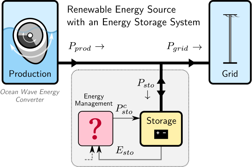
Figure 1: Power smoothing with an Energy Storage: an example of an Optimal Control problem.

1.1 Smoothing with an Energy Storage

Electricity generation from ocean waves (with machines called Wave Energy Converters) is an example where the output power can be strongly fluctuating. This is illustrated on figure 2 where the output power $P_{prod}(t)$ from a particular wave energy converter called SEAREV is represented during 100 seconds.

We just mention that this production time series does not come from measurements but from an hydro-mechanical simulation from colleagues since the SEAREV is a big 1 MW - 30 meters long machine which is yet to be built [Ruellan-2010].

The oscillations of $P_{prod}(t)$ at a period of about 1.5 s comes from the construction of the SEAREV: in short, it is a floating double-pendulum that oscillates with the waves. Also, because ocean waves have a stochastic behavior, the amplitude of these oscillations is irregular.

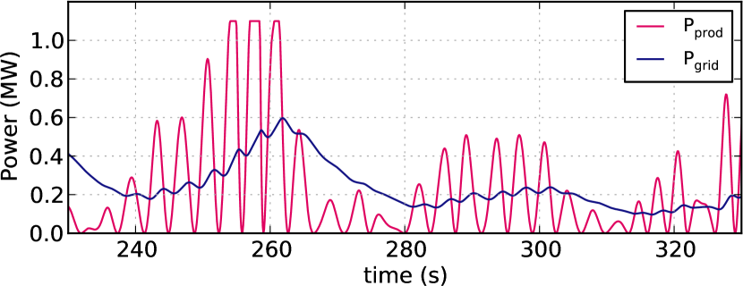
Figure 2: Smoothing the Ocean Power injected to the grid using an Energy Storage controlled by the simple linear law (3). The storage buffers the difference between the two powers.

Therefore an energy storage absorbing a power $P_{sto}$ can be used to smooth out the power $P_{grid}$ injected to the electricity network:

$$P_{grid}(t)=P_{prod}(t)-P_{sto}(t)$$ (1)

The energy of the storage then evolves as:

$$E_{sto}(k+1)=E_{sto}(k)+P_{sto}(k)\Delta t$$ (2)

expressed here in discrete time ($\Delta t=0.1\text{ s}$ throughout this article), without accounting for losses. The storage energy is bounded: $0\leq E_{sto}\leq E_{rated}$, where $E_{rated}$ denotes the storage capacity which is set to 10 MJ in this article (i.e. about 10 seconds of reserve at full power)

It is a control problem to choose a power smoothing law. We present the example of a linear feedback control:

$$P_{grid}(t)=\frac{P_{max}}{E_{rated}}E_{sto}(t)$$ (3)

where $P_{max}$ is the rated power of the SEAREV (1.1 MW). This law gives “good enough” smoothing results as it can be seen on figure 2.

The performance of the smoothing is greatly influenced by the storage sizing (i.e. the choice of the capacity $E_{rated}$). This question is not addressed in this article but was discussed by colleagues [Aubry-2010]. We also don’t discuss the choice of the storage technology, but it is believed that super-capacitors would be the most suitable choice. Because energy storage is very expensive (~20 k€/kWh or ~5 k€/MJ for supercaps), there is an interest in studying how to make the best use of a given capacity to avoid a costly over-sizing.

1.2 Finding an Optimal Smoothing Policy

Control law (3) is an example of heuristic choice of policy and we now try to go further by finding an optimal policy.

Optimality will be measured against a cost function $J$ that penalizes the average variability of the power injected to the grid:

$$J=\frac{1}{N}\mathbb{E}\left\{\sum_{k=0}^{N-1}c(P_{grid}(k))\right\}\quad\text{with $N\rightarrow\infty$}$$ (4)

where $c$ is the instantaneous cost (or penalty) function which can be $c(P_{grid})=P_{grid}^{2}$ for example. Expectation $\mathbb{E}$ is needed because the production $P_{prod}$ is a stochastic input, so that the output power $P_{grid}$ is also a random variable.

This minimization problem falls in the class of stochastic dynamic optimization. It is dynamic because decisions at each time-step cannot be taken independently due to the coupling along time introduced by the evolution of the stored energy (2). To describe the dynamics of the system, we use the generic notation

$$x_{k+1}=f(x_{k},u_{k},\varepsilon_{k})$$ (5)

where $x,u,\varepsilon$ are respectively state variables, control variables and perturbations. State variables are the “memory” of the system. The stored energy $E_{sto}$ is here the only state variable, but more will appear in section 2.2. Control variables are the ones which values must be chosen at each instant to optimize the cost $J$. The injected power $P_{grid}$ is here the single control variable.

Dynamic optimization (also called optimal control) is addressed by the Dynamic Programming method [Bertsekas-2005] which yields a theoretical analysis of the solution structure. Indeed, once all state variables (i.e. “memories”) of the system are identified, the optimum of the cost $J$ is attained by a “state feedback” policy, that is a policy where the control is chosen as a function of the state:

$$P_{grid}(t)=\mu(x(t))$$ (6)

The goal is then to find the optimal feedback function $\mu$. Since $E_{sto}$ is a state variable, policy (3) is in fact a special case of (6). Since $\mu$ has no special structure in the general case¹, it will be numerically computed on a grid over the state space. We cover the algorithm for this computation in section 3.

1.2.1 Prerequisite

Dynamic Programming does require that stochastic perturbations are independent random variables (i.e. the overall dynamical model must be Markovian) and this is not true for the $P_{prod}(k)$ time series. Therefore we devote section 2 to the problem of expressing $P_{prod}$ as a discrete-time Markov process, using time series analysis. This will yield new state variables accounting for the dynamics of $P_{prod}$.

2 Stochastic Model of a Wave Energy Production

We now take a closer look at the $P_{prod}$ time series. A 1000 s long simulation is presented on figure 4, along with a zoom to better see the structure at short time scales. An histogram is also provided which shows that $P_{prod}$ is clearly non-gaussian. This precludes the direct use of “standard” time series models based on Autoregressive Moving Average (ARMA) models [Brockwell-1991].

However, we can leverage the knowledge of the inner working of the SEAREV. Indeed, by calling $\Omega$ the rotational speed of the inner pendulum with respect to the hull, we know that the output power is:

$$P_{prod}=T_{PTO}(\Omega).\Omega$$ (7)

where $T_{PTO}$ is the torque applied to the pendulum by the electric machine which harvests the energy (PTO stands for “Power Take Off”). Finding the best $T_{PTO}$ command is actually another optimal control problem which is still an active area of research in the Wave Energy Conversion community [Kovaltchouk-2013]. We use here a “viscous damping law, with power leveling”, that is $T_{PTO}(\Omega)=\beta.\Omega$. This law is applied as long as it yields a power below $P_{max}$. Otherwise the torque is reduced to level the power at 1.1 MW as can be seen on figure 4 whenever the speed is more than 0.5 rad/s.

Thanks to equation (7), we can thus model the speed $\Omega$ and then deduce $P_{prod}$. Modeling the speed is much easier because it is quite Gaussian (see fig. 4) and has a much more regular behavior which can be captured by an ARMA process.

2.1 Autoregressive Model of the Speed

Within the ARMA family, we restrict ourselves to the autoregressive (AR) processes because we need a Markovian model. The equation of an AR(p) model for the speed is:

$$\Omega(k)=\phi_{1}\Omega(k-1)+\dots+\phi_{p}\Omega(k-p)+\varepsilon(k)$$ (8)

where $p$ is the order of the model and $\varepsilon(k)$ is a series independent random variables. Equation (8) indeed yields a Markovian process, using the lagged observations of the speed $\Omega(k-1),\dots,\Omega(k-p)$ as state variables.

AR(p) model fitting consists in selecting the order $p$ and estimating the unknown coefficients $\phi_{1},\dots,\phi_{p}$ as well as the unknown variance of $\varepsilon$ which we denote $\sigma_{\varepsilon}^{2}$.

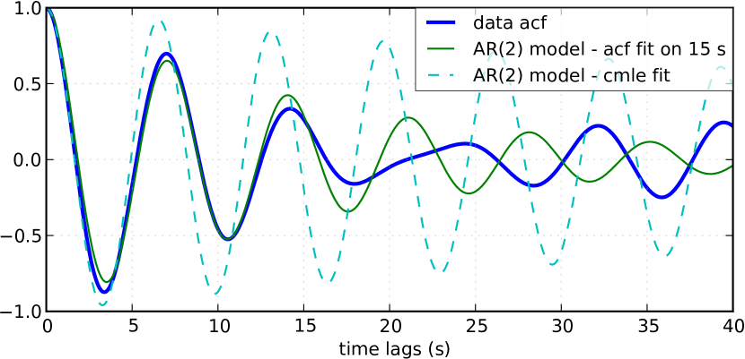
Figure 3: Autocorrelation function (acf) of the speed data, compared with the acf from two AR(2) models, fitted with two different methods.

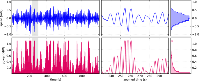
Figure 4: Speed & Power time series from a 1000 seconds SEAREV simulation (sample Em_1.txt). The gray rectangle time interval is enlarged in the middle panel. Distribution histogram on the right.

2.1.1 Order selection

is generally done using information criterions such as AIC or BIC [Brockwell-1991], but for this modeling problem, we restrict ourselves to the smallest order which can reproduce the decaying oscillations of the autocorrelation function. Autocorrelation (acf) of the speed is plotted on figure 3 where we can see that a model of order $p=2$ can indeed reproduce the autocorrelation up to about 15 s of time lags (a 1^st order model would only yield an exponential decay without oscillations). 15 s is thought to be the time horizon of interest when using a 10 MJ/1.1 MW energy storage.

Keeping the model order low is required to maintain the dimension of the overall state vector under 3 or 4. The underlying issue of an exponentially growing complexity will appear in section 3 when solving the Dynamic Programming equation.

2.1.2 Parameter estimation

Once the order is selected, we have to estimate coefficients $\phi_{1}$, $\phi_{2}$ and $\sigma_{\varepsilon}^{2}$. “Classical” fitting methodology [Brockwell-1991] is based on Conditional Maximum Likelihood Estimators (CMLE). This method is readily available in GNU R with the arima routine or in Python with statsmodel.tsa.ar_model.

However, we have plotted the autocorrelation of the estimated AR(2) model on figure 3 to show that CMLE is not appropriate: oscillations of the acf clearly decay too slowly compared to the data acf.

The poor adequacy of this fit is actually a consequence of our choice of a low order model which implies that the AR(2) process can only be an approximation of the true process. Statistically speaking, our model is misspecified, whereas CMLE is efficient for correctly specified models only. This problem has been discussed in the literature [McElroy-2013] and has yielded the “Multi-step ahead fitting procedure”.

Being unfamiliar with the latter approach, we compute instead $\phi_{1},\phi_{2}$ estimates which minimize the difference between the theoretical AR(2) acf and the data acf. The minimization criterion is the sum of the squared acf differences over a range of lag times which can be chosen. We name this approach the “multi-lags acf fitting” method. Minimization is conducted with fmin from scipy.optimize.

method	$\hat{\phi}_{1}$	$\hat{\phi}_{2}$	$\hat{\sigma}_{\varepsilon}$
CMLE	1.9883 (.0007)	-0.9975 (.0007)	0.00172
fit on 15 s	1.9799	-0.9879	0.00347

TABLE II: AR(2) fitting results from the two methods (along with standard error when available).

The result of this acf fitting over time lags up to 15 s (i.e. 150 lags) is shown on figure 3 while numerical estimation results are given in table I.

With the model obtained from this multi-lags method, we can simulate speed and power trajectories and check that they have a “realistic behavior”. We can thus infer that the dynamic optimization algorithm should make appropriate control decisions out of it. This will be discussed in section 3.3. Going further, it would be interesting to study the influence of the AR parameters (including order $p$) on the dynamic optimization to see if the “multi-lags acf fitting” indeed brings an improvement of the final cost function $J$.

2.2 Reformulation as a state-space model

The AR(2) model is a state-space model with state variables being the lagged observations of the speed $\Omega(k-1)$ and $\Omega(k-2)$. In order to get a model with a better “physical interpretation” we introduce the variable $A_{k}=(\Omega_{k}-\Omega_{k-1})/\Delta t$ which is the backward discrete derivative of $\Omega$. As the timestep gets smaller $A_{k}$ comes close to the acceleration (in rad/s²) of the pendulum. Using $(\Omega,A)$ as the state vector, we obtain the following state-space model:

$$\begin{split}\begin{pmatrix}\Omega_{k}\\ A_{k}\end{pmatrix}=&\begin{bmatrix}\phi_{1}+\phi_{2}&-\phi_{2}\Delta t\\ (\phi_{1}+\phi_{2}-1)/\Delta t&-\phi_{2}\end{bmatrix}\begin{pmatrix}\Omega_{k-1}\\ A_{k-1}\end{pmatrix}\\ +&\begin{bmatrix}1\\ 1/\Delta t\end{bmatrix}\varepsilon_{k}\end{split}$$ (9)

We now have a stochastic Markovian model for the power production of the SEAREV. Taken together with state equation of the storage (2) and algebraic relations (1) and (7), we have a Markovian model of the overall system. The state vector $x=(E_{sto},\Omega,A)$ is of dimension 3 which is just small enough to apply the Stochastic Dynamic Programming method.

3 Optimal storage control with Dynamic Programming

3.1 The Policy Iteration Algorithm

We now give an overview of the policy iteration algorithm that we implemented to solve the power smoothing problem described in the introduction. Among the different types of dynamic optimization problems, it is an “infinite horizon, average cost per stage problem” (as seen in (4)). While at first this cost equation involves a summation over an infinite number of instants, the Dynamic Programming approach cuts this into two terms: the present and the whole future. In the end, the optimization falls back to solving this equilibrium equation:

$$\begin{split}J+\tilde{J}(x)=\min_{u\in U(x)}\underset{w}{\mathbb{E}}\Big{\{}\underbrace{c(x,u,w)}_{\text{instant cost}}\\ +\underbrace{\tilde{J}(f(x,u,w))}_{\text{cost of the future}}\Big{\}}\end{split}$$ (10)

where $J$ is the minimized average cost and $\tilde{J}$ is the transient (or differential) cost function, also called value function.

Note that eq. (10) is a functional equation for $\tilde{J}$ which should be solved for any value of the state $x$ in the state space. In practice, it is solved in a discrete grid that must be chosen so that the variations of $\tilde{J}$ are represented with enough accuracy. Also, the optimal policy $\mu$ appears implicitly as the argmin of this equation, that is the optimal control $u$ for each $x$ value of the state grid.

3.1.1 Equation solving

The simplest way to solve eq. (10) is to iterate the right-hand side, starting with a zero value function. This is called value iteration.

A more efficient approach is policy iteration. It starts with an initial policy (like the heuristic linear (3)) and gradually improves it with a two steps procedure:

• policy evaluation: the current policy is evaluated, which includes computing the average cost (4) and the so-called value function

• policy improvement: a single step of optimization with policy iteration yields a improved policy. Then this policy must be again evaluated (step 1).

The policy evaluation involves solving the equilibrium equation without the minimization step but with a fixed policy $\mu$ instead:

$$\begin{split}J_{\mu}+\tilde{J}_{\mu}(x)=\underset{w}{\mathbb{E}}\Big{\{}\underbrace{c(x,\mu(x),w)}_{\text{instant cost}}\\ +\underbrace{\tilde{J}_{\mu}(f(x,\mu(x),w))}_{\text{cost of the future}}\Big{\}}\end{split}$$

It can be solved by iterating the right-hand side like for policy iteration but much faster due to the absence of minimization. In the end, a few policy improvement iterations are needed to reach convergence. More details about the value and policy iteration algorithms can be found in [Bertsekas-2005] textbook for example. The conditions for the convergence, omitted here, are also discussed.

3.2 StoDynProg library description

We have created a small library to describe and solve optimal control problems (in discrete time) using the Stochastic Dynamic Programming (SDP) method. It implements the value iteration and policy iteration algorithms introduced above. Source code is available on GitHub https://github.com/pierre-haessig/stodynprog under a BSD 2-Clause license.

3.2.1 Rationale for a library, benefits of Python

Because the SDP algorithms are in fact quite simple (they can be written with one set of nested for loops) we were once told that they should be written from scratch for each new problem. However we face in our research in energy management several optimization problems with slight structural differences so that code duplication would be unacceptably high. Thus the motivation to write a unified code that can handle all our use cases, and hopefully some others’.

StoDynProg is pure Python code built with numpy for multi-dimensional array computations. We also notably use an external multidimensional interpolation routine by Pablo Winant (see 3.2.5 below).

The key aspect of the flexibility of the code is its ability to handle problems of arbitrary dimensions (in particular the state space and the control space). This impacts particularly the way to iterate over those variables. Our code makes thus a heavy use of Python tuple packing/unpacking machinery and itertools.product to iterate on rectangular grids of arbitrary dimension.

3.2.2 API description

StoDynProg provides two main classes: SysDescription and DPSolver.

3.2.3 SysDescription

holds the description of the discrete-time dynamic optimization problem. Typically, a user writes its dynamics function (the Python implementation of $f$ in (5)) and handles it to a SysDescription instance:

from stodynprog import SysDescription# SysDescription object with proper dimensions# of state (2), control (1) and perturbation (1)mysys = SysDescription((2, 1, 1))def my_dyn(x1, x2, u, w):    ’dummy dynamics’    x1_next = x1 + u + w    x2_next = x2 + x1    return (x1_next, x2_next)# assign the dynamics function:mysys.dyn = my_dynWe use here a setter/getter approach for the dyn property. The same is used to describe the cost function ($c$ in (4)). We believe the property approach enables simplified user code compared to a class inheritance mechanism. With some inspiration of Enthought traits, the setter has a basic validation mechanism that checks the signature of the function being assigned (with getargspec from the inspect module).

3.2.4 DPSolver

holds parameters that tunes the optimization process, in particular the discretized grid of the state. Also, it holds the code of the optimization algorithm in its methods. We illustrate here the creation of the solver instance attached to the previous system:

from stodynprog import DPSolver# Create the solver for ‘mysys‘ system:dpsolv = DPSolver(mysys)# state discretizationx1_min, x1_max, N1 = (0, 2.5, 100)x2_min, x2_max, N2 = (-15, 15, 100)x_grid = dpsolv.discretize_state(x1_min, x1_max, N1,                                 x2_min, x1_max, N2)Once the problem is fully described, the optimization can be launched by calling dpsolv.policy_iteration with proper arguments about the number of iterations.

For more details on StoDynProg API usage, an example problem of Inventory Control is treated step-by-step in the documentation (created with Sphinx).

3.2.5 Multidimensional Interpolation Routine

StoDynProg makes an intensive use of a multidimensional interpolation routine that is not available in the “standard scientific Python stack”. Interpolation is needed because the algorithm manipulates two scalar functions which are discretized on a grid over the state space: the value function $\tilde{J}$ and feedback policy $\mu$. Thus, functions are stored as $n$-d arrays, where $n$ is the dimension of the state vector ($n=3$ for ocean power smoothing example). In the course of the algorithm, the value function needs to be evaluated between grid points, thus the need for interpolation.

3.2.6 Requirements and Algorithm Selection

No “fancy” interpolation method is required so linear interpolation is a good candidate. Speed is very important because it is called many times. Also, it should accept vectorized inputs, so that interpolation of multiple points can be done efficiently in one call. We assert that the functions will be stored on a rectangular grid which should simplify interpolation computations. The most stringent requirement is multidimensionality (for $0\leq n\leq 4$) which rules out most available tools.

We have evaluated 4 routines (details available in an IPython Notebook within StoDynProg source tree):

• LinearNDInterpolator class from scipy.interpolate

• RectBivariateSpline class from scipy.interpolate

• map_coordinates routine from scipy.ndimage

• and MultilinearInterpolator class written by Pablo Winant within its Dolo project [Winant-2010] for Economic modelling (available on https://github.com/albop/dolo).

The most interesting in terms of performance and off-the-shelf availability is RectBivariateSpline which exactly meets our needs expect for multidimensionality because it’s limited to $n=2$. LinearNDInterpolator has no dimensionality limitations but works with unstructured data and so does not leverage the rectangular structure. Interpolation time was found 4 times longer in 2D, and unacceptably long in 3D. Then map_coordinates and MultilinearInterpolator were found to both satisfy all our criterions but the latter being consistently 4 times faster (both 2D and 3D case). Finally we also selected MultilinearInterpolator because it can be instantiated to retain the data once and then called several time. We find the usage of this object-oriented interface more convenient than functional interface of map_coordinates.

3.3 Results for Searev power smoothing

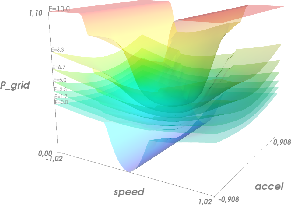
Figure 5: Storage control policy: Power injected to the grid as a function of speed and acceleration, for 7 levels of stored energy between empty and full.

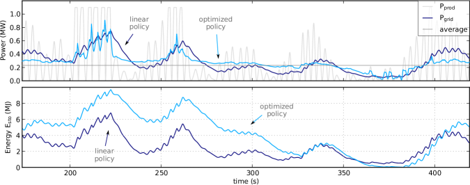
Figure 6: Comparison of the power smoothing behavior between the heuristic (dark blue) and optimized (light blue) storage management policies (storage capacity of 10 MJ). Stored energy on the bottom panel.

We have applied the policy iteration algorithm to the SEAREV power smoothing problem introduced in section 1. The algorithm is initialized with the linear storage control policy (3). This heuristic choice is then gradually improved by each policy improvement step.

3.3.1 Algorithm parameters

About 5 policy iterations only are needed to converge to an optimal strategy. In each policy iteration, there is a policy evaluation step which requires 1000 iterations to converge. This latter number is dictated by the time constant of the system (1000 steps $\leftrightarrow$ 100 seconds) and 100 seconds is the time it takes for the system to “decorrelate”, that is loose memory of its state (both speed and stored energy).

We also need to decide how to discretize and bound the state space of the {SEAREV + storage} system:

• for the stored energy $E_{sto}$, bounds are the natural limits of the storage: $E_{sto}\in[0,E_{rated}]$. A grid of 30 points yields precise enough results.

• for the speed $\Omega$ and the acceleration $A$, there are no natural bounds so we have chosen to limit the values to $\pm 4$ standard deviations. This seems wide enough to include most observations but not too wide to keep a good enough resolution. We use grids of 60 points to keep the grid step small enough.

This makes a state space grid of $30\times 60\times 60\approx 110\text{k}$ points. Although this number of points can be handled well by a present desktop computer, this simple grid size computation illustrates the commonly known weakness of Dynamic Programming which is the “Curse of Dimensionality”. Indeed, this size grows exponentially with the number of dimensions of the state so that for practical purpose state dimension is limited to 3 or 4. This explains the motivation to search a low order model for the power production time series in section 2.

3.3.2 Algorithm execution time

With the aforementioned discretization parameters, policy evaluation takes about 10 s (for the 1000 iterations) while policy improvement takes 20 s (for one single value iteration step). This makes 30 s in total for one policy iteration step, which is repeated 5 times. Therefore, the optimization converges in about 3 minutes. This duration would grow steeply should the grid be refined.

As a comparison of algorithm efficiency, the use of value iteration would takes much longer than policy iteration. Indeed, it needs 1000 iterations, just like policy evaluation (since it is dictated by the system’s “decorrelation time”) but each iteration involves a costly optimization of the policy so that it takes 20 s. This makes altogether 5 hours of execution time, i.e. 100 times more than policy iteration!

As possible paths to improve the execution time, we see, at the code level, the use of more/different vectorization patterns although vectorized computation is already used a lot. Maybe the use of Cython may speed up unavoidable loops but this may not be worth the loss of flexibility and the decrease in coding speed. Optimization at the algorithm level, just as demonstrated with “policy vs. value iteration”, is also worth investigating further. In the end, more use of Robert Kern’s line_profiler will be needed to decide the next step.

3.3.3 Output of the computation

The policy iteration algorithm solves equation (10) and outputs the minimized cost $J$ and two arrays: function $\tilde{J}$ (transient cost) and function $\mu$ (optimal policy (6)), both expressed on the discrete state grid (3d grid).

We focus on $\mu$ which yields the power $P_{grid}$ that should be injected to the grid for any state of the system. Figure 5 is a Mayavi surface plot which shows $P_{grid}(\Omega,A)$ for various levels of $E_{sto}$. Observations of the result are in agreement with what can be expected from a reasonable storage control:

• the more energy there is in the storage, the more power should be injected to the grid (similar to the heuristic control (3)).

• the speed and acceleration of the SEAREV also modulates the injected power, but to a lesser extent. We may view speed and acceleration as approximate measurements of the mechanical energy of the SEAREV. This energy could be a hidden influential state variable, in parallel with the stored energy.

• the injected power is often set between 0.2 and 0.3 MW, that is close to the average power production.

Such observations show that the algorithm has learned from the SEAREV behavior to take sharper decisions compared to the heuristic policy it was initialized with.

3.3.4 Qualitative analysis of the trajectory

To evaluate the storage control policy, we simulate its effect on the sample SEAREV data we have (instead of using the state space model used for the optimization). The only adaptation required for this trajectory simulation is to transform the policy array ($\mu$ known on the state grid only) into a policy function ($\mu$ evaluable on the whole state space). This is achieved using the same n-dimensional interpolation routine used in the algorithm.

A simulated trajectory is provided on figure 6 to compare the effect of the optimized policy with the heuristic linear policy (3). As previously said, the storage capacity is fixed at $E_{rated}=10\text{ MJ}$ or about 9 seconds of charge/discharge at the rated power.

Positive aspect, the optimized policy yields an output power that is generally closer to the average (thin gray line) than the linear policy. This better smoothing of the “peaks and valleys” of the production is achieved by a better usage of the available storage capacity. Indeed, the linear policy generally under-uses the higher levels of energy.

As a slight negative aspect, the optimized policy yields a “spiky” output power in the situations of high production (200–220 s). In this situation, the output seems worse that the linear policy. We connect this underperformance to the linear model (9) used to represent the SEAREV dynamics. The linearity holds well for small movements but not when the speed is high and the pendulum motion gets very abrupt (acceleration high above 4 standard deviations which contradicts the Gaussian distribution assumption). Since the control optimization is based on the linear model, the resulting control law cannot appropriately manage these non-linear situations. Only an upgraded model would genuinely solve this problem but we don’t have yet an appropriate low-order non-linear model of the SEAREV. One quick workaround to reduce the power peaks is to shave the acceleration measurements (not demonstrated here).

3.3.5 Quantitative assessment

We now numerically check that the optimized policy brings a true enhancement over the linear policy. We simulate the storage with the three 1000 s long samples we have and compute the power variability criterion² for each.

Figure 7 shows the standard deviation for each sample in three situations: without storage (which yields the natural standard deviation of the SEAREV production), with a storage controlled by the linear policy and finally the same storage controlled by the optimized policy. Sample Em_1.txt was used to fit the state space model (9) but we don’t think this should introduce a too big bias because of the low model order.

Beyond the intersample variability, we can see the consistent improvement brought by the optimized law. Compared to the linear policy, the standard deviation of the injected power is reduced by about 20 % (27 %, 16 %, 22 % for each sample respectively). We can conclude that the variability of the injected power is indeed reduced by using the Dynamic Programming.

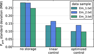
Figure 7: Effect of optimizing the storage control on three SEAREV production time series. Standard deviation compared to the heuristic linear control case is reduced by about 20 %.

Because the RMS deviation criterion used in this article is not directly limited or penalized in current grid codes, there is no financial criterion to decide whether the observed deviations are acceptable or not. Therefore we cannot conclude if the ~20% reduction of the variability brought by optimal control is valuable. Nevertheless, there exists criterions like the "flicker" which are used in grid codes to set standards of power quality. Flicker, which is way more complicated to than an additive criterion like (4) could be used to put an economic value on a control strategy. This is the subject of ongoing research.

4 Conclusion

With the use of standard Python modules for scientific computing, we have created StoDynProg, a small library to solve Dynamic Optimization problems using Stochastic Dynamic Programming.

We have described the mathematical and coding steps required to apply the SDP method on an example problem of realistic complexity: smoothing the output power of the SEAREV Wave Energy Converter. With its generic interface, StoDynProg should be applicable to other Optimal Control problems arising in Electrical Engineering, Mechanical Engineering or even Life Sciences. The only requirement is an appropriate mathematical structure (Markovian model), with the “Curse of Dimensionality” requiring a state space of low dimension.

Further improvements on this library should include a better source tree organization (make a proper package) and an improved test coverage.

References

- [Aubry-2010] J. Aubry, P. Bydlowski, B. Multon, H. Ben Ahmed, and B. Borgarino. Energy Storage System Sizing for Smoothing Power Generation of Direct Wave Energy Converters, 3rd International Conference on Ocean Energy, 2010.
- [Bertsekas-2005] D. P. Bertsekas, Dynamic Programming and Optimal Control, Athena Scientific, 2005.
- [Brockwell-1991] P. J. Brockwell, and R. A. Davis. Time Series: Theory and Methods, Springer Series in Statistics, Springer, 1991.
- [Kovaltchouk-2013] T. Kovaltchouk, B. Multon, H. Ben Ahmed, F. Rongère, J. Aubry, and A. Glumineau. Influence of control strategy on the global efficiency of a Direct Wave Energy Converter with electric Power Take-Off, EVER 2013 conference, 2013.
- [McElroy-2013] T. McElroy, and M. Wildi. Multi-step-ahead estimation of time series models, International Journal of Forecasting, 29: 378–394, 2013.
- [Ruellan-2010] M. Ruellan, H. Ben Ahmed, B. Multon, C. Josset, A. Babarit, and A. Clément. Design Methodology for a SEAREV Wave Energy Converter, IEEE Trans. Energy Convers, 25: 760–767, 2010.
- [Winant-2010] P. Winant. Dolo, a python library to solve global economic models, http://albop.github.io/dolo, 2010.