Pipe Poiseuille flow of viscously anisotropic, partially molten rock

Abstract

Laboratory experiments in which synthetic, partially molten rock is subjected to forced deformation provide a context for testing hypotheses about the dynamics and rheology of the mantle. Here our hypothesis is that the aggregate viscosity of partially molten mantle is anisotropic, and that this anisotropy arises from deviatoric stresses in the rock matrix. We formulate a model of pipe Poiseuille flow based on theory by Takei and Holtzman (2009a) and Takei and Katz (2013). Pipe Poiseuille is a configuration that is accessible to laboratory experimentation but for which there are no published results. We analyse the model system through linearised analysis and numerical simulations. This analysis predicts two modes of melt segregation: migration of melt from the centre of the pipe toward the wall and localisation of melt into high-porosity bands that emerge near the wall, at a low angle to the shear plane. We compare our results to those of Takei and Katz (2013) for plane Poiseuille flow; we also describe a new approximation of radially varying anisotropy that improves the self-consistency of models over those of Takei and Katz (2013). This study provides a set of baseline, quantitative predictions to compare with future laboratory experiments on forced pipe Poiseuille flow of partially molten mantle.

1 Introduction

Partially molten regions of the mantle are inaccessible to direct observations, making it difficult to validate theoretical models for their mechanics. Laboratory experiments performed on synthetic mantle rocks represent a valuable alternative to direct observations. In laboratory experiments, when partially molten mantle rocks are deformed to large strains, bands of high and low volume-fraction of melt (porosity) emerge spontaneously and remain oriented at a low angle of $\sim$15–20^∘ to the shear plane (e.g. King et al., 2010).

Modelling this pattern-forming instability is recognised as a means to validate theoretical models of magma/mantle interaction, regardless of whether the same instability occurs in Earth’s mantle. Stevenson (1989) described a one-dimensional model that was the first to predict the instability under a porosity-weakening aggregate viscosity; this work preceded and motivated the laboratory experiments. Extension to a two-dimensional theory by Spiegelman (2003) predicted porosity band emergence at 45^∘ to the shear plane. Katz et al. (2006) obtained theoretical models of low-angle bands by extending the porosity-weakening viscosity to be strongly non-Newtonian. However, direct measurements by King et al. (2010) of the stress dependence of the aggregate viscosity in band-forming experiments were much lower than required by Katz et al. (2006), falsifying their model. Evidently, although the governing equations permit formation of high-porosity bands, the details of the pattern depend on the features of the rheology that is assumed.

In the models noted above, the viscosity of the grain$+$melt aggregate was assumed isotropic but this need not be the case. Takei and Holtzman (2009a, b) developed a theory for viscous anisotropy of a partially molten aggregate in which the anisotropy arises from the grain-scale distribution of melt. If the aggregate deforms in diffusion creep and the melt provides a fast pathway for diffusion of grain material, then a coherent alignment of melt pockets at the micro-scale will give rise to faster and slower directions for diffusive response to deviatoric stress at the macro-scale. According to Takei and Holtzman (2009a) and Takei (2010), melt-filled pores preferentially align normal to the direction of largest tensile stress, which reduces the aggregate viscosity to deformation in the same direction. On this basis, Takei and Holtzman (2009a) and Takei and Katz (2013) formulated a viscosity tensor for the two-phase aggregate. Analysis of this tensor by Takei and Holtzman (2009c), Butler (2012), Takei and Katz (2013), and Katz and Takei (2013) shows that it leads to a prediction of low-angle porosity bands, consistent with laboratory experiments.

In laboratory experiments reported by Holtzman et al. (2003), Holtzman and Kohlstedt (2007), King et al. (2010), and Qi et al. (2013b), the synthetic rocks subjected to deformation are aggregates of $\sim$10 $\mu$m mantle olivine and chromite grains, plus 2–5 vol% basalt or anorthite powder. The material is raised to a pressure of 300 MPa and temperature of $\sim$1200^∘C, under which conditions the basalt or anorthite is molten and resides within the pores between the solid grains of olivine and chromite. The samples are held at these conditions until they reach textural equilibrium, with an approximately uniform porosity throughout the sample. They are then deformed at strain rates of $\sim$10^-4 sec^-1 by application of a deviatoric stress. The samples are quenched after reaching a predetermined maximum strain, sectioned, and analysed for the resulting porosity distribution. Early experiments by Holtzman et al. (2003) and Holtzman and Kohlstedt (2007) were performed in simple-shear geometry, which imparts an obvious limitation on the total strain that can be achieved. Deformation in torsion was achieved later (King et al., 2010; Qi et al., 2013b) and allows (in theory) for unlimited amounts of strain.

Both simple shear and torsional deformation were considered in the theoretical work of Takei and Katz (2013) and Katz and Takei (2013). Under simple shear, leading-order flow is lateral and leading-order stress is initially uniform throughout the experiment. Under torsional deformation, the leading-order flow is in the azimuthal direction around a cylinder; the deviatoric stress is zero at the centre of the cylinder and largest at the outer radius, giving a gradient directed radially outward. Takei and Katz (2013) found that with the inclusion of anisotropic viscosity, this gradient in deviatoric stress drives melt migration toward the centre of the cylinder, independent of any initial porosity variations. To elucidate this prediction of “base state segregation,” they considered a third configuration, plane Poiseuille flow. In Poiseuille flow, there is gradient in shear stress from zero at the centre of the flow to a maximum at the outer edge, where the aggregate abuts the fixed walls. The geometrical contrast between plane Poiseuille and torsional deformation enabled Takei and Katz (2013) to resolve the forces driving melt segregation and make quantitative predictions of base state segregation. These predictions are testable for torsional flow, and indeed early results indicate agreement with theory (Qi et al., 2013a; Katz et al., 2013).

Predictions of melt segregation under plane Poiseuille flow are not readily testable because this configuration is difficult to implement in the laboratory. Pipe Poiseuille, however, is an accessible alternative. It is therefore the goal of the present manuscript to apply the formulation of Takei and Katz (2013) for anisotropic viscosity of a partially molten aggregate to the geometry of pipe Poiseuille flow. Moreover, the results of such calculations may be relevant to magma transport within the stem of a mantle plume or a crystal-rich volcanic conduit, though we do not explore these applications here. Below we reintroduce the theory and provide new solutions in cylindrical geometry. We address the inconsistencies in the analysis by Takei and Katz (2013) and generate models that are more physically and mathematically consistent.

The manuscript is organised as follows. The governing equations are presented in the next section, followed by a linearised stability analysis in section 3. In section 3.1 we consider the leading-order, base state dynamics for spatially uniform and radially variable anisotropy, and then compare the results to plane Poiseuille. In section 3.2 we calculate the growth rate of band-like porosity perturbations. We return to the base state in section 4 but consider solutions to the fully nonlinear governing equations. We discuss our results in light of previous theoretical and experimental work in section 5 and provide a summary and conclusions in 6.

2 Governing Equations

Here we consider a formulation of the equations for coupled magma/mantle deformation that was presented by Takei and Katz (2013). This formulation differs from other recent versions (e.g. Bercovici et al., 2001; Rudge et al., 2011; Keller et al., 2013) in that it allows for an anisotropic relationship between stress and strain rate.

2.1 Conservation statements

The full system of conservation equations consists of two statements of conservation of mass and two statements of conservation of momentum. These are described by Takei and Katz (2013) and can be solved for the volume fraction of liquid $\phi(\boldsymbol{x},t)$, solid and liquid velocity fields $\boldsymbol{v}^{S}(\boldsymbol{x},t)$ and $\boldsymbol{v}^{L}(\boldsymbol{x},t)$, and liquid pressure $p^{L}$. It is convenient to manipulate the equations to eliminate $\boldsymbol{v}^{L}$, resulting in the system

$$\dfrac{\partial{\phi}}{\partial{t}} =\nabla\cdot\left[(1-\phi)\boldsymbol{v}^{S}\right],$$ (1a)

$$\boldsymbol{\nabla}\cdot\boldsymbol{v}^{S} =\boldsymbol{\nabla}\cdot\left[\frac{K}{\eta^{L}}\left(\boldsymbol{\nabla}p^{L}-\rho^{L}\boldsymbol{g}\right)\right],$$ (1b)

$$\dfrac{\partial{p^{L}}}{\partial{x_{i}}} =\dfrac{\partial{}}{\partial{x_{j}}}\left(\sigma_{ij}+p^{L}\delta_{ij}\right)+\overline{\rho}g_{i},$$ (1c)

where $K=K(\phi)$ is the permeability, $\eta^{L}$ is the liquid viscosity, $\boldsymbol{g}$ is the vector acceleration of gravity, $\sigma_{ij}$ is the stress tensor of the solid+liquid aggregate (tension positive), and $\rho^{L},\overline{\rho}$ are the liquid and aggregate densities. The first equation represents mass conservation for the solid phase under the assumption of constant solid density; the second equation is derived from force balance in the liquid phase; the third equation is force balance for the two-phase aggregate. We take $\rho^{L}=\rho^{S}=\overline{\rho}=\rho=\text{const.}$ in what follows. We furthermore take $\eta^{L}$, and $\boldsymbol{g}$ to be constant and uniform.

Although we do not solve for the velocity of the liquid explicitly, it can be obtained directly by substitution of the solution of (1) into the conservation of momentum equation for the liquid, which is a modified version of Darcy’s law (e.g., Takei and Katz, 2013).

Here we are concerned with the forced flow of the two-phase aggregate through a cylindrical pipe with a diameter that is much larger than the grain size of the solid mantle rock. It is therefore convenient to write the equations in cylindrical polar coordinates $(r,\psi,z)$, defined so that $\boldsymbol{g}=-g\hat{\boldsymbol{z}}$ and the axis of the cylinder lies along the $z$-axis at $r=0$,

$$\dfrac{\partial{\phi}}{\partial{t}} =\frac{1}{r}\dfrac{\partial{}}{\partial{r}}\left[r(1-\phi)v_{r}\right]+\dfrac{\partial{}}{\partial{z}}\left[(1-\phi)v_{z}\right],$$ (2a)

$$\frac{1}{r}\dfrac{\partial{}}{\partial{r}}(rv_{r})+\dfrac{\partial{v_{z}}}{\partial{z}} =\frac{1}{r}\dfrac{\partial{}}{\partial{r}}\left(r\frac{K}{\eta^{L}}\dfrac{\partial{p^{L}}}{\partial{r}}\right)+\dfrac{\partial{}}{\partial{z}}\left[\frac{K}{\eta^{L}}\left(\dfrac{\partial{p^{L}}}{\partial{z}}+\rho g\right)\right],$$ (2b)

$$\dfrac{\partial{p^{L}}}{\partial{r}} =\dfrac{\partial{}}{\partial{r}}\left(\sigma_{rr}+p^{L}\right)+\frac{\sigma_{rr}-\sigma_{\psi\psi}}{r}+\dfrac{\partial{}}{\partial{z}}\sigma_{rz},$$ (2c)

$$\dfrac{\partial{p^{L}}}{\partial{z}} =\dfrac{\partial{}}{\partial{r}}\sigma_{rz}+\frac{\sigma_{rz}}{r}+\dfrac{\partial{}}{\partial{z}}\left(\sigma_{zz}+p^{L}\right)-\rho g.$$ (2d)

Here we have assumed azimuthal symmetry ($\partial(\cdot)/\partial\psi=0$), zero azimuthal velocity ($v_{\psi}=0$), and used $\boldsymbol{v}^{S}=(v_{r},0,v_{z})$. Under this coordinate system and state of symmetry, the strain-rate tensor for the solid phase is

$$\dot{\varepsilon}_{ij}=\bordermatrix{~{}&r&\psi&z\cr r&\dfrac{\partial{v_{r}}}{\partial{r}}&0&\dfrac{1}{2}\left(\dfrac{\partial{v_{r}}}{\partial{z}}+\dfrac{\partial{v_{z}}}{\partial{r}}\right)\cr\psi&0&\dfrac{v_{r}}{r}&0\cr z&\dfrac{1}{2}\left(\dfrac{\partial{v_{r}}}{\partial{z}}+\dfrac{\partial{v_{z}}}{\partial{r}}\right)&0&\dfrac{\partial{v_{z}}}{\partial{z}}}.$$ (3)

2.2 Constitutive relations

Closure of the system of partial differential equations (2) requires that we specify a relationship between permeability $K$ and porosity $\phi$, and a relationship between the bulk stress tensor $\sigma_{ij}$ and the solid strain-rate tensor $\dot{\varepsilon}_{ij}$. For the former we make the canonical choice appropriate at small porosity,

$$K(\phi)=K_{0}\left({\phi}/{\phi_{0}}\right)^{n},$$ (4)

where $n$ is a constant, usually taken as two or three, and $\phi_{0}$ is a reference porosity at which the permeability takes its reference value $K_{0}$ (McKenzie, 1989; Riley and Kohlstedt, 1991; Faul, 1997; Wark and Watson, 1998).

Following on the work of Takei and Katz (2013), we can relate the second-order stress tensor to the second-order strain-rate tensor via a fourth-order viscosity tensor,

$$\sigma_{ij}+p^{L}\delta_{ij}=c_{ijkl}\dot{\varepsilon}_{kl},$$ (5)

where $\delta_{ij}$ is the identity tensor. Takei and Holtzman (2009a, b) developed a microstructural model for diffusion creep of a partially molten rock to relate the macroscopic stress tensor to the viscosity tensor. They predicted a transversely isotropic viscosity with rotational symmetry about the axis of maximum tension (the $\sigma_{3}$-direction) and anisotropic weakening along this axis; they further predicted that the magnitude of this anisotropy is a bounded function of the stress anisotropy, $(\sigma_{3}-\sigma_{1})$.

Consistent with our requirement of azimuthal symmetry of the flow, we assume that the principal axes of the stress tensor corresponding to the minimum and maximum tensile stress ($\sigma_{1}$ and $\sigma_{3}$, respectively) lie in the $z$–$r$ plane of the cylindrical coordinate system for any azimuth $\psi$. On this basis, we specify the orientation of the anisotropy tensor as the angle $\Theta$ between the $z$-axis and the direction of maximum tensile stress. Following Takei and Katz (2013) in defining $\alpha$ as the magnitude of anisotropy and requiring $0\leq\alpha\leq 2$, we can write the anisotropy tensor as

$$c_{ijkl}=\eta_{0}\text{e}^{-\lambda(\phi-\phi_{0})}\times\bordermatrix{~{}&rr&\psi\psi&zz&r\psi&\psi z&zr\cr rr&B&C&A&0&0&-D\cr\psi\psi&C&C+2&C&0&0&0\cr zz&A&C&F&0&0&-E\cr r\psi&0&0&0&1&0&0\cr\psi z&0&0&0&0&1&0\cr zr&-D&0&-E&0&0&A-C+1},$$ (6)

where $\lambda$ is a constant, typically taken in the range 25–30, and we have defined

$$A =r_{\xi}-{2}/{3}-\alpha\cos^{2}\Theta\sin^{2}\Theta,$$ (7)

$$B =r_{\xi}+{4}/{3}-\alpha\sin^{4}\Theta,$$

$$C =r_{\xi}-{2}/{3},$$

$$D =\alpha\cos\Theta\sin^{3}\Theta,$$

$$E =\alpha\cos^{3}\Theta\sin\Theta,$$

$$F =r_{\xi}+{4}/{3}-\alpha\cos^{4}\Theta.$$

In this set of equations, $r_{\xi}$ is the bulk-to-shear viscosity ratio. The remaining components of $c_{ijkl}$ follow by symmetry of the tensor. The tensor $c_{ijkl}$ is identical to that used by Takei and Katz (2013) (their eqn. 4.9) with the relabelling of coordinates $Z\rightarrow\psi$, $X\rightarrow z$, and $Y\rightarrow r$. It is important to note that anisotropy ($\alpha>0$) introduces coupling between shear stresses and normal strain-rates (and, by symmetry, normal stresses and shear strain-rates). When $\alpha=0$, the viscosity tensor reduces to its standard, isotropic form and this coupling vanishes.

For all calculations in the present manuscript we take $n=3$, $\phi_{0}=0.05$, $\lambda=27$, and $r_{\xi}=5/3$. The value for $r_{\xi}$ was obtained by Takei and Holtzman (2009a) through microstructural modelling; the value for $\lambda$ fits experimental data (Kelemen et al., 1997) and is consistent with the same microstructural model; the value for $n$ is taken to be $3$ for consistency with previous studies and based on Wark and Watson (1998) (note, however that the permeability exponent was recently estimated by Miller et al. (2014) as $2.6\pm 0.2$ on the basis of simulated flow through pore networks obtained by three-dimensional micro-tomographic scans of texturally equilibrated olivine and basalt.)

2.3 Scaling and non-dimensionalisation

Let $H$ be the radius of the cylinder; a typical rate of vertical, solid-phase flow through the cylinder is then $U=\rho gH^{2}/\eta_{0}$. We use these to introduce rescaled, dimensionless variables as follows:

$\boldsymbol{X}=\dfrac{\boldsymbol{x}}{H}$,	$\boldsymbol{V}=\dfrac{\boldsymbol{v}^{S}}{U}$,	$K^{*}=\dfrac{K}{K_{0}}=\left(\dfrac{\phi}{\phi_{0}}\right)^{n}$,
$\sigma^{*}_{ij}=\dfrac{\sigma_{ij}+p^{L}\delta_{ij}}{\left({\eta_{0}U}/{H}\right)}$,	$P=\dfrac{p^{L}}{\rho gH}$,	$\dot{\varepsilon}^{*}_{ij}=\dfrac{\dot{\varepsilon}_{ij}}{\left({U}/{H}\right)}$ ,
$c^{*}_{ijkl}=\dfrac{c_{ijkl}}{\eta_{0}}$,	$\tau=\dfrac{t}{\left({H}/{U}\right)}$.

We will break with the notation defined above, however, and refer to the non-dimensional radial and vertical coordinates as $r$ and $z$, respectively, for the rest of the manuscript.

In writing the non-dimensional equations, it is convenient to define a ratio of the compaction length, an inherent length scale of magma/mantle interaction (McKenzie, 1984), to the system size $H$,

$$R=\dfrac{1}{H}\sqrt{\dfrac{(r_{\xi}+\frac{4}{3})\eta_{0}K_{0}}{\eta^{L}}}.$$ (8)

Liquid pressure perturbations cause variations in melt flux (and hence (de)compaction) over a length scale that is less than or equal to the compaction length (Spiegelman, 1993). Hence we expect the compaction length to influence the scale of emergent features in the solution.

The governing equations, expressed in terms of non-dimensional quantities, are

$$\frac{\partial\phi}{\partial\tau} =\nabla\cdot\left[(1-\phi)\boldsymbol{V}\right],$$ (9a)

$$\nabla\cdot\boldsymbol{V} =\frac{R^{2}}{r_{\xi}+{4}/{3}}\nabla\cdot\left[K^{*}(\nabla P+\hat{\boldsymbol{z}})\right],$$ (9b)

$$\frac{\partial P}{\partial r} =\dfrac{\partial{}}{\partial{r}}\sigma^{*}_{rr}+\frac{\sigma^{*}_{rr}-\sigma^{*}_{\psi\psi}}{r}+\dfrac{\partial{}}{\partial{z}}\sigma^{*}_{rz},$$ (9c)

$$\frac{\partial P}{\partial z} =\dfrac{\partial{}}{\partial{r}}\sigma^{*}_{rz}+\frac{\sigma^{*}_{rz}}{r}+\dfrac{\partial{}}{\partial{z}}\sigma^{*}_{zz}-1.$$ (9d)

Components of the non-dimensional stress tensor are given by

$$\sigma_{ij}^{*}=\text{e}^{-\lambda(\phi-\phi_{0})}\begin{cases}AV_{z,z}+BV_{r,r}+C{V_{r}}/{r}-D\left(V_{z,r}+V_{r,z}\right)&ij=rr,\\[5.69054pt] CV_{z,z}+CV_{r,r}+(C+2)V_{r}/r&ij=\psi\psi,\\[5.69054pt] FV_{z,z}+AV_{r,r}+C{V_{r}}/{r}-E\left(V_{z,r}+V_{r,z}\right)&ij=zz,\\[5.69054pt] -EV_{z,z}-DV_{r,r}+(A-C+1)\left(V_{z,r}+V_{r,z}\right)&ij=rz.\end{cases}$$ (10)

This formulation is valid for radially variable anisotropy parameters $\alpha$ and $\Theta$, which give rise to radially variable coefficients $A,B,D,E,F$.

2.4 Boundary condition

The pipe wall at $r=1$ is modelled as a no-slip, impermeable, rigid boundary with $V_{r}=V_{z}=0$. At the centre line $r=0$, we require that the solution is non-singular, which leads to the symmetry conditions $V_{r}=V_{z,r}=P_{,r}=0$. We assume an infinitely long pipe, and hence for the unperturbed base state, we exclude all variation in the $z$-direction (except for periodic solutions). Finally, since the pressure is only constrained up to an additive constant, we choose that $P=0$ at $r=0$ (without loss of generality).

3 Analysis

Various authors have employed a linearisation of the governing equations to study the small-time evolution of porosity that results from forced deformation. Spiegelman (2003) and Katz et al. (2006), for example, considered the stability of plane-wave perturbations to porosity under a forced, simple-shear flow. Takei and Holtzman (2009c) and Butler (2012) extended this analysis to consider anisotropic viscosity as formulated by Takei and Holtzman (2009a). This was further extended by Takei and Katz (2013) to investigate the consequences of anisotropic viscosity under three flow configurations: simple shear, plane Poiseuille, and torsion. Below we compare our results with their solutions for plane Poiseuille flow.

The strategy for analysis, in all of these studies, is to expand the solution in a power series of a small parameter $\epsilon\ll 1$, substitute into the governing equations, and balance terms in $\epsilon^{0}$ and $\epsilon^{1}$ separately. Here we use

$$\phi =\phi_{0}+\epsilon\phi_{1}+O(\epsilon^{2}),$$ (11)

$$P =P_{0}+\epsilon P_{1}+O(\epsilon^{2}),$$

$$\boldsymbol{V} =\boldsymbol{V}^{(0)}+\epsilon\boldsymbol{V}^{(1)}+O(\epsilon^{2}),$$

$$\mathcal{C} =\mathcal{C}_{0}+\epsilon\mathcal{C}_{1}+O(\epsilon^{2}),$$

where we have defined the compaction rate as $\mathcal{C}\equiv\boldsymbol{\nabla}\cdot\boldsymbol{V}$. The leading-order terms are called the base state and the first-order terms are the perturbations.

3.1 The base state

The base state is initialised with a uniform porosity $\phi_{0}$. Under isotropic viscosity ($\alpha=0$), this base state porosity remains constant with time. However, under anisotropic viscosity ($0<\alpha\leq 2$) and with a spatially varying stress field, we expect that the base state porosity will evolve in the radial direction, similar to plane Poiseuille flow (Takei and Katz, 2013). Hence the base state variables will depend on $r$ and time $\tau$, but will be independent of $z$. We seek the instantaneous solution at $\tau=0$, when the porosity is uniform and the base state permeability is unity.

The leading-order balances in equations (9b) and (9c) can be combined to eliminate the radial pressure gradient and then integrated to give

$$V^{(0)}_{r}=\frac{R^{2}}{r_{\xi}+{4}/{3}}\left[\dfrac{\partial{}}{\partial{r}}\left(B\dfrac{\partial{V^{(0)}_{r}}}{\partial{r}}+C\frac{V^{(0)}_{r}}{r}-D\dfrac{\partial{V_{z}^{(0)}}}{\partial{r}}\right)+\frac{B-C}{r}\dfrac{\partial{V^{(0)}_{r}}}{\partial{r}}-2\frac{V^{(0)}_{r}}{r^{2}}-\frac{D}{r}\dfrac{\partial{V_{z}^{(0)}}}{\partial{r}}\right];$$ (12a)

radial integration of equation (9d) gives

$$-D\dfrac{\partial{V^{(0)}_{r}}}{\partial{r}}+(A-C+1)\dfrac{\partial{V^{(0)}_{z}}}{\partial{r}}=\frac{r}{2}.$$ (12b)

Here we have used the boundary conditions and enforced no singularity at $r=0$.

Given an anisotropy field in terms of $\alpha$ and $\Theta$, equations (12) can be solved for the base state flow at $\tau=0$. We consider two models for the distribution of anisotropy. The first assumes that anisotropy is uniform (Takei and Katz, 2013). The second model uses a pre-computed, radial variation of $\alpha$ and $\Theta$ that is based on a hypothesis for the dynamic control of anisotropy. For the constant-anisotropy case, we compare solutions for pipe Poiseuille with those for plane Poiseuille flow obtained by Takei and Katz (2013).

3.1.1 Uniform anisotropy

For an isotropic system, the base state velocity field $\boldsymbol{V}^{(0)}$ is identical to that of single-phase, incompressible, Stokes flow in the same geometry. It is only for non-zero $\alpha$ that the dynamics lead to divergent solid velocity and hence radial compaction.

The simplest model for the distribution of non-zero anisotropy is constant $\alpha$ and $\Theta$; this condition was employed by Takei and Katz (2013). Uniform anisotropy allows for an analytical solution to (12), which we detail in appendix A. However, this solution (and the uniform anisotropy condition itself) violates the expected symmetry of the problem and leads to a mathematical and physical singularity. We present examples of the solution nonetheless, for comparison with previous work and because they are instructive.

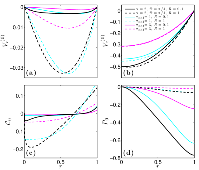
Figure 1: Radial profiles of base state variables for uniform anisotropy (black curves; $\alpha=2,\;\Theta=\pi/4$) and radially-variable anisotropy (cyan and magenta curves; equations (16)–(18)). (a) Radial component of the solid velocity $V_{r}^{(0)}$. (b) Vertical component of the solid velocity $V_{z}^{(0)}$. (c) Compaction rate $\mathcal{C}_{0}$. (d) Pressure $P_{0}$.

Black lines in Figure 1 show the base state solution at $\tau=0$ under uniform anisotropy. Two representative values of the dimensionless compaction length are used. For $R>1$, the solutions have the same radial structure and saturate at only slightly larger amplitude than for $R=1$. For $R<0.1$, the boundary layers narrow and the solution amplitude is reduced. Panel a shows the radial component of the velocity; all values are negative, indicating solid motion toward the centre of the cylinder. For small compaction length, there are narrow boundary layers near the centre and wall of the cylinder, whereas for large compaction length, the radial component varies throughout the domain. These features are mirrored in panel c, showing the compaction rate. All curves show that there is compaction (and hence decreasing porosity) near the centre of the cylinder and decompaction near the wall. For small compaction length, there is a range of radii between the compaction boundary layers where $\mathcal{C}_{0}$ is approximately zero, while for large compaction length, $\mathcal{C}_{0}$ crosses zero at a point.

Figure 1c also shows that for constant anisotropy, $\mathcal{C}_{0}$ has a singular derivative at $r=0$ (black curves). The symmetry of the physical problem should lead to the requirement that $\partial\mathcal{C}_{0}/\partial r=0$ at the centre of the cylinder and, in fact, that $\mathcal{C}_{0}$ should be an even function of $r$. With the constant anisotropy assumption, this criterion is not met and the radial derivative of the compaction rate is singular at the centre of the cylinder.

The problem of $\mathcal{C}_{0}$ having a singularity at the centre is also discernable in both the plane Poiseuille and the torsion analysis of Takei and Katz (2013), respectively resulting from the assumptions of non-zero $\Theta$ and non-zero $\alpha$ at the origin. For torsion and plane Poiseuille, as for pipe Poiseuille, the horizontal velocity equation under the uniform anisotropy assumption has a non-smooth solution (see Takei and Katz, 2013).

Another consideration in evaluating the uniform-anisotropy model is how well it approximates what it is intended to: the radial variation in dynamic, stress-induced anisotropy as proposed by Takei and Katz (2013). The angle of anisotropy should be defined by the direction of maximum tensile stress; the magnitude of anisotropy should approach zero as the magnitude of stress approaches zero. Takei and Katz (2013) proposed a theory for the dependence of $\alpha$ on the components of the stress tensor, but that theory is fundamentally nonlinear and not easily incorporated in our analysis. Therefore, in the next section, we impose $\alpha$ and $\Theta$ a priori, as explicit functions of radius. These functions are chosen such that they are in approximate agreement with the retrieved variation of $\alpha$ and $\Theta$, which is computed a posteriori from the base state solution.

3.1.2 Non-uniform anisotropy

The model for stress-dependent anisotropy presented in Takei and Katz (2013) is defined by the following expressions, from which we determine $\alpha$ and $\Theta$:

$$\cos(2\Theta) =\frac{\sigma_{zz}-\sigma_{rr}}{\sigma_{3}-\sigma_{1}},\quad\sin(2\Theta)=\frac{2\sigma_{rz}}{\sigma_{3}-\sigma_{1}},$$ (13a)

$$\alpha =2\tanh\left(\frac{2(\sigma_{3}-\sigma_{1})}{\sigma_{\text{sat}}}\right),$$ (13b)

where $\sigma_{\text{sat}}$ is a material parameter and $\sigma_{1}\leq 0$ and $\sigma_{3}\geq 0$ are the values of the principal stresses (tension positive). Equations (13) give

$$\alpha =2\tanh\left(\frac{4\sigma_{rz}}{\sigma_{\text{sat}}\sin(2\Theta)}\right)=2\tanh\left(\frac{2(\sigma_{zz}-\sigma_{rr})}{\sigma_{\text{sat}}\cos(2\Theta)}\right),$$ (14)

$$\Theta =\frac{1}{2}\arg(2\sigma_{rz}i+\sigma_{zz}-\sigma_{rr}),$$ (15)

in terms of the entries of the stress tensor expressed in system coordinates. Here and below, “$\arg$” is the argument of the complex number, and takes values in the range $(-\pi,\pi]$.

Figure 2a–b show a comparison of imposed (uniform) anisotropy with the retrieved variation in anisotropy computed by substituting the stress tensor from the base state solution into (14) and (15). Focusing attention on $\Theta$ in panel b, we see that for the case of $R=0.1$, there is a region of approximate consistency between the imposed and retrieved anisotropy, but for $R=1$ there is not. So we see that beyond the need for a distribution of anisotropy that respects the symmetry conditions of the problem, an imposed anisotropy distribution should be approximately consistent with the consequent base state distribution of stress.

One way to achieve such consistency is by fixed-point iteration: imposing the retrieved anisotropy to recompute the flow and then iterating this process until the difference between anisotropy at subsequent iterations is below a specified tolerance. However, we are interested in obtaining approximate analytical forms that may be less accurate but are of greater utility for subsequent analysis. Below we propose a priori radial forms of $\alpha$ and $\Theta$ to substitute into the equations, with the aim of achieving the desired consistency. Specifying the forms of $\alpha$ and $\Theta$ before solving the differential equations preserves the linearity of the differential equations in $V^{(0)}_{r}$ and $V^{(0)}_{z}$.

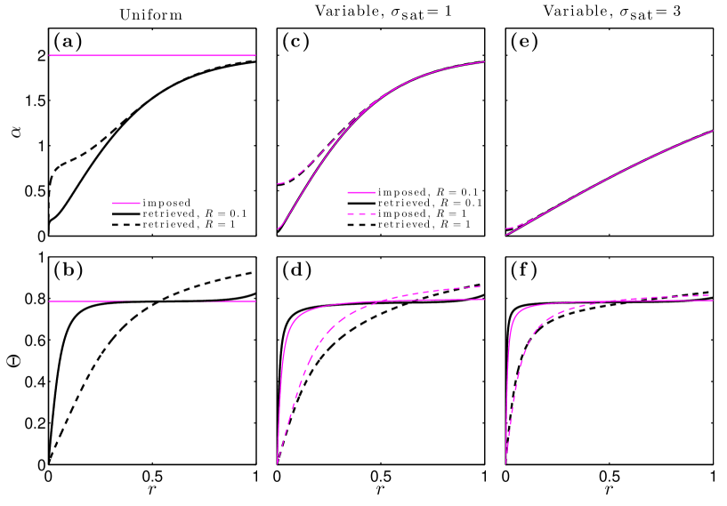
Figure 2: Imposed and retrieved anisotropy parameters $\alpha$ (top row) and $\Theta$ (bottom row). Retrieved means computed by inserting the radial solution for $\boldsymbol{{V}^{(0)}}$ into equations (14) and (15). The first column has imposed uniform anisotropy with $\alpha=2,\;\Theta=\pi/4$; the second and third columns have variable anisotropy imposed with equations (16)–(18) and with $\sigma_{\text{sat}}$ of 1 and 3, respectively.

A reasonable level of consistency can be achieved with a model of the form

$$\Theta =\frac{1}{2}\arg\left[ri+f_{1}(r)\right],\quad\alpha=2\tanh\left[f_{2}(r)\right],$$ (16)

$$\text{with}\quad f_{1}(r) =m_{1}(1-2r)\quad\text{and}\quad f_{2}(r)=\frac{2r}{\sigma_{\text{sat}}}+m_{2}\exp\left(-\frac{2r}{m_{2}\sigma_{\text{sat}}}\right),$$ (17)

where $m_{1}$ and $m_{2}$ are constants that may depend on $R$ and $\sigma_{\text{sat}}$. For large ranges of $R$ and $\sigma_{\text{sat}}$, suitable expressions for the constants $m_{1}$ and $m_{2}$ are

$$m_{1} =\tanh R\times\left[0.3\exp\left(-0.6\sigma_{\text{sat}}\right)+0.03\right],$$ (18a)

$$m_{2} =2m_{1}/\sigma_{\text{sat}}.$$ (18b)

Note that these expressions for the anisotropy parameters satisfy $\Theta=0$ and $\partial\alpha/\partial r=0$ at the centre of the cylinder and we therefore expect the corresponding solution to be more regular there. However, for an anisotropy model that is completely smooth at $r=0$ (and hence a completely smooth solution), we would require $f_{1}$ and $f_{2}$ to be even functions of $r$.

Solutions of equations (12) incorporating radial variation in anisotropy are obtained numerically, to a tolerance of $10^{-10}$, using the Chebfun package (Driscoll et al., 2008; Trefethen et al., 2011; Trefethen, 2013) for Matlab.

Figure 1a–b show the components of base state velocity under an imposed, radially variable anisotropy (coloured curves). These differ quantitatively from the uniform anisotropy case, but the qualitative pattern is unchanged. The base state velocity solutions can be used to compute a dynamic anisotropy (eqns. (14) and (15)) to compare with the imposed anisotropy as a check for self-consistency.

Figure 2c–f illustrates the self-consistency of the anisotropy model defined by equations (16)–(18). It shows that for a range of $R$ and $\sigma_{\text{sat}}$, the pre-computed anisotropy that is imposed on the model is approximately consistent with that computed using the solution. Also it shows that the models for $\alpha(r)$ and $\Theta(r)$ satisfy $\partial\alpha/\partial r=\Theta=0$ at $r=0$.

Figure 1c shows the base state compaction rate $\mathcal{C}_{0}$ for uniform and radially variable anisotropy. For $R=0.1$, the compaction boundary layer near $r=0$ disappears under variable anisotropy in favour of a broad, compacting region over most of the domain. Evidently the solutions with variable anisotropy satisfy the condition of zero radial derivative of compaction at the centre of the cylinder. Having achieved both consistency and sufficient regularity, we conclude that the chosen forms of $f_{1}$, $f_{2}$, $m_{1}$, and $m_{2}$ are reasonable approximations, and a significant improvement over uniform anisotropy.

A remaining question about the radially variable model for imposed anisotropy is how well it agrees with solutions of the full, nonlinear system of equations with dynamic anisotropy given by (14) and (15). This comparison is performed below in section 4, which regards numerical solutions to the governing equations. We find excellent agreement at $\tau=0$ when the numerical model is initialised with uniform porosity.

3.1.3 Comparison with the plane Poiseuille base state

Takei and Katz (2013) obtained an analytical solution for the base state solid velocity at $\tau=0$ under conditions of plane Poiseuille flow with uniform anisotropy (constant $\alpha$ and $\Theta=\pi/4$). For a channel of half-width $H$, the solution can be non-dimensionalised with the characteristic speed $U=\rho gH^{2}/\eta_{0}$ for comparison with pipe Poiseuille. This solution is given in terms of non-dimensional quantities on $0\leq x\leq 1$ as

$$V^{(0)}_{x}= \frac{R^{2}\alpha}{(r_{\xi}+4/3)(4-\alpha)}\left(\frac{\sinh\>[\beta x/R]}{\sinh\>[{\beta}/{R}]}+\frac{\sinh\>[{\beta(1-x)}/{R}]}{\sinh\>[{\beta}/{R}]}-1\right),$$ (19a)

$$V^{(0)}_{z}= \frac{2(x^{2}-1)}{4-\alpha}+\frac{\alpha}{4-\alpha}\left(V^{(0)}_{x}-(x-1)\left.V^{(0)}_{x,x}\right|_{x=0}\right),$$ (19b)

where

$$\beta=\sqrt{\dfrac{r_{\xi}+\frac{4}{3}}{r_{\xi}+\frac{4}{3}-\frac{\alpha}{4-\alpha}}}.$$

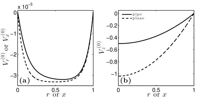
Figure 3: Comparison of base state velocity for pipe and plane Poiseuille geometry. Both are computed for uniform anisotropy ($\alpha=2,\;\Theta=\pi/4$) and $R=0.1$. (a) Radial or lateral component of the velocity. (b) Vertical component.

Takei and Katz (2013) assumed constant anisotropy parameters $\alpha$ and $\Theta$, so for the purpose of comparison, we have used our own constant anisotropy solution for pipe Poiseuille, with the identical parameter values. Therefore both the planar and cylindrical solutions have physical inconsistencies at the centre, but their comparison nevertheless demonstates a broad similarity between the flows, and suggests how they scale relative to each other.

Figure 3 shows profiles of solid velocity components for plane Poiseuille flow, plotted alongside profiles for pipe Poiseuille flow with uniform anisotropy. The vertical velocity components have the same shape, but differ by a factor of two in magnitude; this is what we would expect from the analytical solutions to single phase, isoviscous Poiseuille flow in the two flow geometries. The horizontal components are also similar in shape, and as $R$ increases the horizontal flow in cylindrical geometry becomes smaller relative to that in planar geometry. However, for $R\lesssim 0.1$, the horizontal velocities are approximately equal in magnitude, as shown in figure 3a. In other words, for these smaller values of $R$, if we normalise by the magnitude of the vertical flow, we predict stronger lateral flow in the cylindrical geometry.

3.2 Growth of porosity perturbations

Having obtained solutions for the base state variables, we now turn our attention to the terms of order $\epsilon$ in equations (11). These represent perturbations to the base state; we will analyse them by seeking harmonic solutions that can grow or decay exponentially with time. There is no universally accepted method for analysing the linear stability of a time-dependent base state (Doumenc et al., 2010). For simplicity, we consider perturbation growth only at $\tau=0$, and therefore take $\phi_{0}$ to be constant and uniform in solving for the evolution of perturbations. The calculations in this section are valid for uniform and radially variable anisotropy.

Equations to constrain the $O(\epsilon)$ terms are obtained by substituting the expansion (11) into the governing equations (9). The leading-order terms already balance and the terms of $O(\epsilon^{2})$ can be neglected, leaving equations for $\partial\phi_{1}/\partial\tau$, $P_{1}$, and $\boldsymbol{V}^{(1)}$; these equations are given in Appendix B. We consider porosity perturbations of the form

$$\phi_{1}(r,z,\tau)=\exp\left[i\boldsymbol{k}\cdot\left(\boldsymbol{x}-\int\limits_{0}^{\tau}{\boldsymbol{V}^{(0)}}\mathrm{d}t\right)+\Psi(r,z,\tau)\right],$$ (20)

where the wave-vector is $\boldsymbol{k}=k_{r}\hat{\boldsymbol{r}}+k_{z}\hat{\boldsymbol{z}}$ with $k_{r}$ and $k_{z}$ constants. Equation (20) represents cones of locally harmonic waves moving passively in the base state flow $\boldsymbol{V}^{(0)}$ with a time-dependent log-amplitude $\Psi$; the tips of the cones are located at $r=0$ and point upward for $k_{r},k_{z}>0$. We define

$$k \equiv\sqrt{k_{r}^{2}+k_{z}^{2}},$$ (21)

$$s+i\Omega \equiv\frac{\partial\Psi}{\partial\tau},$$ (22)

$$\text{and we require}\quad\nabla\Psi\text{, }\nabla(s+i\Omega) =o(k)\text{ as }k\rightarrow\infty,$$ (23)

where a quantity $q$ that is $o(k)$ satisfies $q/k\rightarrow 0$ as $k\rightarrow\infty$. The last equation states that both $\Psi$ and the growth rate of porosity perturbations $s+i\Omega$ are slowly varying in space, in the sense that they vary on a length scale that is much longer than the wavelength of perturbations. Because the governing system is linear at each order of $\epsilon$, we can relate other variables to $\phi_{1}$ as

$$\boldsymbol{V}^{(1)}=\tilde{\boldsymbol{V}}\phi_{1}\text{, }\quad P_{1}=\tilde{P}\phi_{1},$$ (24)

with $\tilde{V_{r}}$, $\tilde{V_{z}}$, and $\tilde{P}$ also only slowly varying. In the following analysis we do not perturb the quantities $A$ to $F$; the analysis is therefore suitable for $\alpha$ and $\Theta$ either constant or specified a priori, but not dynamically variable.

Fixing $\tau=0$, taking $k\rightarrow\infty$, and neglecting all but terms of leading order in $k$, the equations can be inverted to give expressions for $\tilde{V_{r}}$, $\tilde{V_{z}}$, and $\tilde{P}$ that are valid to leading order in $k$. Then, to obtain the growth rate, we use (9a) at $O(\epsilon)$ leading to

$$s+i\Omega\sim(1-\phi_{0})\left(ik_{r}\tilde{V_{r}}+ik_{z}\tilde{V_{z}}\right)-\nabla\cdot\boldsymbol{V}^{(0)}$$ (25)

as $k\rightarrow\infty$ (here and below we use the symbol $\sim$ to mean “is asymptotic to.”) Substituting for $ik_{r}\tilde{V_{r}}+ik_{z}\tilde{V_{z}}$ we find that at $\tau=0$ and to leading order in $k$, the growth rate is

$$s\sim\frac{1-\phi_{0}}{N_{3}N_{5}-{N_{4}}^{2}}[(N_{1}N_{5}-N_{2}N_{4})W_{2}+(-N_{1}N_{4}+N_{2}N_{3})W_{3}]-\mathcal{C}_{0}$$ (26)

where

$$N_{1} =ik_{r},$$ (27)

$$N_{2} =ik_{z},$$

$$N_{3} =Bk_{r}^{2}+(A-C+1)k_{z}^{2}-2Dk_{r}k_{z},$$

$$N_{4} =-Dk_{r}^{2}-Ek_{z}^{2}+(2A-C+1)k_{r}k_{z},$$

$$N_{5} =(A-C+1)k_{r}^{2}+Fk_{z}^{2}-2Ek_{r}k_{z},$$

$$W_{2} =-\lambda ik_{r}\left(BV^{(0)}_{r,r}+C{V^{(0)}_{r}}/{r}-DV^{(0)}_{z,r}\right)-\lambda ik_{z}\left[-DV^{(0)}_{r,r}+(A-C+1)V^{(0)}_{z,r}\right],$$

$$W_{3} =-\lambda ik_{r}\left[-DV^{(0)}_{r,r}+(A-C+1)V^{(0)}_{z,r}\right]-\lambda ik_{z}\left(AV^{(0)}_{r,r}+C{V^{(0)}_{r}}/{r}-EV^{(0)}_{z,r}\right).$$

In obtaining this solution we find that $\Omega$ is $o(1)$ as $k\rightarrow\infty$ and, since $s$ is $O(1)$, we have found all the terms of $s+i\Omega$ that do not decay in the $k\rightarrow\infty$ limit of short wavelength. More details of the above calculations are provided in Appendix B.

In the case of isotropic viscosity, the above result (26) for the growth rate $s$ reduces to

$$s\sim\frac{(1-\phi_{0})\lambda rk_{r}k_{z}}{(r_{\xi}+{4}/{3})k^{2}}$$ (28)

as $k\rightarrow\infty$. Let us write

$$\boldsymbol{k}=k(\cos\theta\hat{\boldsymbol{r}}+\sin\theta\hat{\boldsymbol{z}});$$ (29)

then as $k\rightarrow\infty$, the growth rate $s$ is proportional to $\sin(2\theta)$ and so is largest for the perturbations with angle $\theta=45^{\circ}$. This is evident in Figure 4a. The equation for $s(\theta)$ under isotropic viscosity is identical to that obtained for plane Poiseuille flow by Takei and Katz (2013) (up to a scaling constant and replacing $r$ with $Y$).

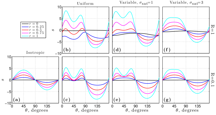
Figure 4: Growth rate $s$ of perturbations as a function of perturbation angle $\theta$ from equation (29). Columns (labelled above) represent different anisotropy scenarios; rows (labelled at right) represent different values of non-dimensional compaction length $R$. (a) $\alpha=0$; (b)–(c) $\alpha=2,\,\Theta=\pi/4$; (d)–(e) $\sigma_{\text{sat}}=1$; (f)–(g) $\sigma_{\text{sat}}=3$. Panels (d)–(g) use radially variable anisotropy $\alpha(r),\Theta(r)$ computed with equations (16). All curves are computed with $\lambda=27,\,\phi_{0}=0.05$.

Figure 4b–c show the growth rate $s$ of perturbations at angle $\theta$ for constant, non-zero anisotropy, given by values of $\Theta={\pi}/{4}$ and $\alpha=2$. Clearly $45^{\circ}$ is no longer the most favourable angle for growth. Focusing attention on the cyan curves representing band growth at the outer radius of the cylinder, we see that one effect of the anisotropy is to split the single growth rate peak of panel a into two peaks (corresponding to the fastest growing disturbances at $\tau=0$), one at an angle less than $45^{\circ}$ and one at an angle greater than $45^{\circ}$. This effect was also found by Takei and Katz (2013) for plane Poiseuille. Takei and Katz (2013) showed that the positions and relative heights of the two peaks depend on the value of the anisotropy angle $\Theta$. In the case $\Theta={\pi}/{4}$, the peaks occur at angles of approximately $15^{\circ}$ and $75^{\circ}$. For values of constant $\Theta$ less than ${\pi}/{4}$, the low-angle peak is dominant, and occurs at an angle larger than $15^{\circ}$.

The uniform anisotropy calculations in Figure 4b–c also show a clear trend with radius. Growth rates are fastest for low-angle porosity bands located at the outer radius because the strain rate is largest there. The shear strain rate goes to zero at the centre of the cylinder and hence we expect $s\approx 0$ there (the contributions by $\mathcal{C}_{0}$ and $V^{(0)}_{r,r}$ to $s$ are small but non-zero at $r=0$). However, for antithetical porosity bands ($\theta<90^{\circ}$) at slightly larger radii (e.g., $r=0.25$), we see that the growth rate can be negative, meaning that perturbations decay. This is due to the contribution of base state compaction $\mathcal{C}_{0}$ in eqn. (26). This effect is stronger for $R=1$ because the base state compaction is larger in amplitude (Fig. 1c). For non-dimensional compaction lengths greater than unity, the base state compaction rate saturates in amplitude (Takei and Katz, 2013).

These same effects are evident in panels d–g of Figure 4, where the anisotropy varies radially according to equations (17). For $\sigma_{\text{sat}}=1$, $\alpha$ reaches saturation at the outside of the cylinder, giving large growth rates. In contrast, for $\sigma_{\text{sat}}=3$, anisotropy is relatively muted and hence growth rates are overall smaller and the two peaks merge into a single, broad peak growth rate. The shift from small $\Theta$ at the centre of the cylinder to $\Theta\gtrsim\pi/4$ at the wall can be discerned in panel d, where the low-angle peak is shifted to larger $\theta$ at $r=0.25$ and smaller $\theta$ at $r=1$.

The general systematics of perturbation growth rates are consistent for constant and radially variable anisotropy, as well as for plane and pipe Poiseuille flow. Indeed when we compare equations for the growth rates in plane and pipe flow, we see that differential operators of $\partial_{x}$ for plane flow become $\partial_{r}+r^{-1}$ in pipe flow. When these operators are applied to the perturbation variables in the limit of $k\rightarrow\infty$, the extra term in $r^{-1}$ (coming from the curved geometry) is neglected because it is of a lower order in $k$ than the radial derivative. Nevertheless, there are cylindrical terms (i.e., $V_{r}^{(0)}/r$) that appear in $W_{1}$ and $W_{2}$ (see eqn. (27)), showing that $s$ does depend in some way on the geometry of the flow.

In fact, the most important difference in perturbation growth between pipe and plane Poiseuille comes from the overall scaling of the flows. In this manuscript we scale velocity with $\rho gH^{2}/\eta_{0}$ whereas Takei and Katz (2013) use a value twice as large, $2\rho gH^{2}/\eta_{0}$, reflecting the stronger vertical flow in plane geometry (Fig. 3b, above). This means that our $\tau$ is half that of Takei and Katz (2013). Therefore, although the nondimensional growth rate of perturbations in Figure 4 is approximately equal to that in Figure 9 of Takei and Katz (2013), the dimensional growth rate of perturbations in pipe geometry is about half that of plane geometry, if the pipe and channel have equal diameter and thickness, respectively. This difference arises from the larger vertical shear associated with plane Poiseuille flow (Fig. 3b).

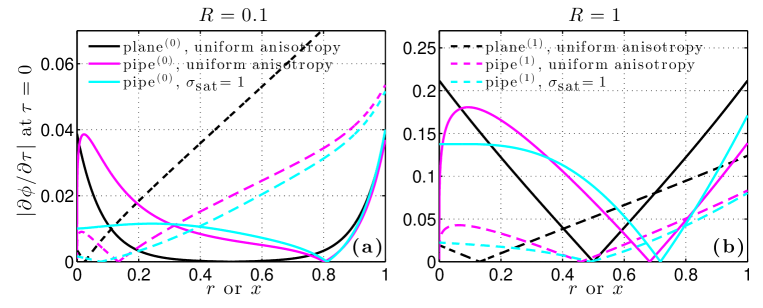
Figure 5: The magnitude of terms in the porosity evolution equation (30). Solid lines show the magnitude of base state segregation $|(1-\phi_{0})\mathcal{C}_{0}|$; dashed lines show the magnitude of the perturbation growth rate $|\epsilon s\phi_{1}|$. Plane Poiseuille with uniform anisotropy is plotted in black as a function of $x$ (scaled with $U=\rho gH^{2}/\eta_{0}$ and computed with $\boldsymbol{V}^{(0)}$ from (19) above). Pipe Poiseuille is plotted in magenta and cyan as a function of $r$, computed with uniform and variable anisotropy, respectively. Pipe and plane flow are computed for a pipe and channel of equal width. The perturbation angle is chosen as $\theta=15^{\circ}$. For uniform anisotropy we use $\alpha=2$ and $\Theta=\pi/4$ while for variable anisotropy we use $\sigma_{\text{sat}}=1$. Other parameter values are $\phi_{0}=0.05$ and $\epsilon=0.2\phi_{0}$. Panel (a) has $R=0.1$; panel (b) has $R=1$.

A more detailed comparison of the rates of base state segregation and perturbation growth is given in Figure 5. This figure shows the magnitude of terms on the right hand side of the porosity evolution equation

$$\dfrac{\partial{\phi}}{\partial{\tau}}=\left(1-\phi_{0}\right)\mathcal{C}_{0}+\epsilon s\phi_{1}.$$ (30)

We expect that the local behaviour of the model is predicted by the term with the larger magnitude. Following Takei and Katz (2013), we take $\epsilon=0.2\phi_{0}$ and consider a fixed perturbation angle $\theta=15^{\circ}$ — this being an optimum value of the growth rate (Fig. 4). The growth rate under plane Poiseuille flow was obtained by Takei and Katz (2013) but here it is scaled by $U/H=\rho gH/\eta_{0}$ (as for pipe flow). The figure predicts that in general, porosity bands are expected to be prominent for small compaction length (panel a) while at larger compaction lengths, base state segregation dominates (panel b).

We can also compare the two modes of segregation for pipe and plane flow. For $R=0.1$ and adjacent to the no-slip wall, pipe and plane flow have approximately equal rates of porosity change due to base state segregation; but through much of the domain, pipe flow has more rapid porosity change by base state segregation. This is in contrast to the rate due to perturbation growth, which is greater for plane Poiseuille throughout the domain. Hence we expect that for small compaction length, high porosity bands are less prominent under pipe Poiseuille flow than under plane Poiseuille. For $R=0.1$ a similar comparison holds, though it is muted: the ratio of magnitude of the two terms on the right-hand side of eqn. (30) is approximately the same for pipe and plane flow.

4 Solutions of the full, nonlinear equations

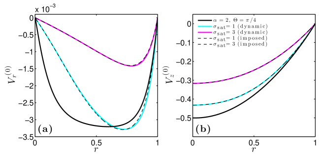
Figure 6: Comparison of radial profiles obtained by solution of the full, nonlinear system with dynamic anisotropy (coloured curves, eqns. (9) & (14)–(15)) to profiles from the base state model with imposed anisotropy (black curves, eqns. (12) & (17)). (a) Radial component of velocity. (b) Vertical component. All calculations use $R=0.1,\,\lambda=27,\,\phi_{0}=0.05,\,n=3$; the fully nonlinear solutions have 400 grid-cells in the radial direction.

For the solutions considered in previous sections, at $\tau=0$ we impose the anisotropy a priori to keep the equations linear. However, equations (14) and (15) provide a recipe for computing the dynamic anisotropy—the pointwise values of $\alpha$ and $\Theta$ that are in equilibrium with the instantaneous stress tensor of the aggregate. This formulation of the viscosity is nonlinear and hence we abandon the linearised governing equations and return to the full, nonlinear system (9). We proceed by discretising the governing equations with a finite volume approximation and solving the resulting system of nonlinear algebraic equations using algorithms provided by the Portable, Extensible Toolkit for Scientific Computation (PETSc, Balay et al., 2001, 2004; Katz et al., 2007). Details are provided in Appendix C.

Although our discretisation and code implementation allow for a two-dimensional ($r$–$z$) domain, we consider only one-dimensional profiles to focus attention on the nonlinear evolution of the base state. The band-forming instability is avoided by considering an initial condition of porosity that is spatially uniform to machine precision. Simulations that are initiated with a small amount of white-noise variation added to the background porosity do produce high porosity bands. As expected from the linearised theory, they are at low angle to the shear direction, appear close to the pipe wall, and are of smaller amplitude than those in plane Poiseuille (Katz and Takei, 2013). These two-dimensional solutions are not reproduced here.

Figure 6 compares one-dimensional solutions to the nonlinear governing equations at $t=0$ with solutions computed using the leading-order equations (12) and imposed anisotropy for $R=0.1$ and $\sigma_{\text{sat}}=1,3$. The excellent match between calculations with dynamic and imposed anisotropy indicates that the numerical solution is accurate (small differences are the result of imperfection in the imposed anisotropy model in equations (16)–(18) with respect to the dynamic determination of self-consistent anisotropy).

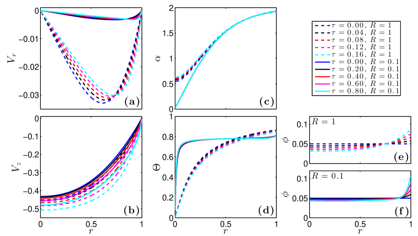
Figure 7: Solutions to the full governing equations at various times $\tau$. (a) Radial component of velocity. (b) Vertical component. (c) Anisotropy magnitude. (d) Anisotropy angle. (e) Porosity for $R=1$. (f) Porosity for $R=0.1$. All calculations use $\lambda=27,\,\phi_{0}=0.05,\,n=3$; the fully nonlinear solutions have 400 grid-cells in the radial direction.

Figure 7 shows the evolution of solutions for $R=0.1$ (solid curves) and $R=1$ (dashed curves) over a finite time interval. The time interval is longer for $R=0.1$ because the radial segregation rate is slower (e.g. Fig. 1c). For both values of the non-dimensional compaction length, however, we see that porosity and shear localise toward the no-slip wall. This was also the case for plane Poiseuille flow (Takei and Katz, 2013). If the simulations are allowed to evolve forward beyond the time interval shown, the porosity continues to localise toward the wall, reducing the aggregate viscosity there. Shear is therefore focused at the wall while strain rates in the interior of the flow decrease. The system rapidly reaches a plug-flow configuration where all deformation is located in a narrow zone of high porosity along the wall. It should be noted, however, that the high porosities reached in this scenario violate assumptions used to derive the governing equations (i.e., that the solid forms a contiguous matrix and that shear stresses in the liquid phase are negligible).

5 Discussion

Pipe Poiseuille flow of a two-phase aggregate with anisotropic viscosity is related to torsional and plane Poiseuille flow, but it differs in important ways. It shares a cylindrical geometry with torsional flow, including base state, compressional hoop stress ($\sigma_{\psi\psi}<0$). In the case of torsional flow (Takei and Katz, 2013), the compressional hoop stress is caused by viscous anisotropy in the tangential ($\psi$–$z$) plane. Both the $\sigma_{1}$ and $\sigma_{3}$ directions lie within this plane (to leading order), in an arrangement that is identical to that of simple shear. The $\sigma_{1}$ (compressional) stress is associated with a large viscosity while the $\sigma_{3}$ (tensile) stress is associated with a reduced viscosity. Hence the imposed shear results in a net compressive stress in the tangential plane: a negative hoop stress. This causes a positive radial pressure gradient (eqn. (9c) above) driving liquid inward (and solid outward).

In contrast, under pipe Poiseuille, the maximum compressive and tensile stresses lie in the $z$–$r$ plane and are the result of the gravitational body force (last term in eqn. (9d) above). These stresses increase in magnitude with $r$. Combined with a tensile viscosity that decreases radially with increasing deviatoric stress, this results in a negative radial pressure gradient. The pressure gradient, in turn, drives liquid outward toward the pipe wall (and solid inward). The compressive hoop stress arises as a consequence of this solid flow ($V_{r}/r<0$). Note the contrast with torsional flow, where the compressive hoop stress is the cause of base state segregation.

We showed above (Fig. 3) that plane and pipe Poiseuille are qualitatively similar in their pattern of base state flow, but differ quantitatively. This is evident especially in the vertical component of the flow, which is slower in cylindrical geometry. This can be understood as being simply related to the mass of aggregate that is supported by a section of the wall of unit length in the cross-flow direction. In plane Poiseuille, the supported material forms a rectangular column, whereas in pipe Poiseuille, the supported material forms a shape like a slice of cake. For a pipe radius equal to the half-width of the plane gap, the rectangular column obviously contains more mass. Given this difference in the vertical component, it is interesting that, for $R\lesssim 0.1$, the horizontal component of the solid velocity is similar in magnitude between pipe and plane Poiseuille. It is also notable that in this range of compaction lengths, where porosity bands are expected to be prominent, pipe flow has weaker band growth relative to base state segregation (Fig. 5).

The time-evolution of porosity under base state segregation brings out a problematic feature of the model: there is no physical mechanism in the theory to balance the accumulation of liquid at the pipe wall. It is possible that such accumulation could occur in experiments, but past experimental works shows that porosities are limited to $\lesssim$25%, even at very large strains (King et al., 2010). This lack of stabilising mechanism in the theory is an issue for all published models of forced, laboratory deformation of partially molten aggregates (though see Takei and Hier-Majumder (2009) for a possible solution).

Our analysis of harmonic perturbations of porosity produced results entirely consistent with previous work on plane Poiseuille by Takei and Katz (2013). Porosity bands are expected to emerge near the pipe wall at angles of $15$–$20^{\circ}$ to the vertical, if anisotropy is at or near saturation. As with previous analysis, the compaction rates associated with band growth must be of the same order or larger than those associated with base state segregation to achieve exponential growth of infinitesimal perturbations (linear instability). Katz and Takei (2013) showed for plane geometry that nonlinear interactions between base state and perturbation flow will modify both modes, but not obscure them entirely. We have not addressed these interactions for pipe flow. Moreover, we have considered only axisymmetric, infinitesimal perturbations, which likely restrict the behavioural space of solutions.

While comparisons with theory for torsional and plane Poiseuille flow elucidate subtleties in the modelled dynamics, comparison with experiments would address a more fundamental question: does outward, base state segregation of liquid occur in synthetic, partially molten mantle rocks subjected to forced flow through a pipe? In experiments, it would be necessary to force the flow with an imposed pressure gradient, rather than with the gravitation body force. Moreover, the finite length of the experimental pipe would introduce complexities not considered here. Far from the ends of the pipe, however, we would expect the predictions developed above to hold, if the aggregate has an anisotropic viscosity similar to the model of Takei and Holtzman (2009a, b) and Takei and Katz (2013).

6 Summary and conclusions

This manuscript considered the problem of gravity-driven flow of a partially molten aggregate through a cylindrical pipe. It presented solutions to the equations thought to govern magma/mantle interaction, incorporating an anisotropic viscosity tensor as a constitutive law for the two-phase flow. These solutions were obtained to zeroth and first order for a linearised version of the equations, as well as to the full, nonlinear system.

As in previous studies, anisotropic viscosity is predicted to lead to melt segregation driven by a gradient in shear stress. For pipe Poiseuille geometry, this means that the liquid is expected to migrate toward the pipe wall, causing decompaction at the outer radii of the flow and compaction at the inner radii. Furthermore, the porosity-weakening of viscosity is expected to give rise to linear instability of bands of high porosity. Our model of anisotropic viscosity indicates that these would take a low angle to the local shear plane. We have noted, however, that band growth in pipe Poiseuille is predicted to be weaker than band growth under plane Poiseuille.

The results presented here are consistent with previous work on anisotropic viscosity, but extend it to pipe Poiseuille flow. This geometry is amenable to laboratory experiments and we hope that future work by experimentalists will evaluate the theory of anisotropic viscosity by testing our predictions. Ideally, a comparison with experiments will yield insights that motivate and constrain refinement of the model.

Acknowledgements

The authors thank Y. Takei for her comments on an early draft and acknowledge two anonymous reviews that helped to improve the manuscript. J.A. was supported by a Research Experience Placement grant from the UK Natural Environment Research Council for Summer 2013. R.K. is grateful for the support of the Leverhulme Trust.

Appendix A Analytical solution for uniform anisotropy base state

With both $\alpha$ and $\Theta$ constant, a suitable transformation puts equation (12a) into the form of a forced, modified Bessel equation of order $\sqrt{(C+2)/[B-D^{2}/(A-C+1)]}$. The solution to this equation that satisfies the boundary condition at $r=1$ and is finite at $r=0$ is given explicitly as

$$V^{(0)}_{r}(r)=\left(\sum_{n=1}^{\infty}a_{n}r^{n}\right)-\frac{I_{\sqrt{\omega_{2}}}(\sqrt{\omega_{1}}r)}{I_{\sqrt{\omega_{2}}}(\sqrt{\omega_{1}})}\left(\sum_{n=1}^{\infty}a_{n}\right),$$ (31)

where $I_{\nu}$ denotes the modified Bessel function of the first kind of order $\nu$ [Baricz, 2010] and

$$a_{n} =\begin{cases}0&\text{for $n$ odd},\\[5.69054pt] \dfrac{\omega_{3}}{4-\omega_{2}}&\text{for $n=2$},\\[11.38109pt] \dfrac{\omega_{1}}{n^{2}-\omega_{2}}a_{n-2}&\text{for $n$ even, $n>2$},\end{cases}$$ (32)

$$\text{and}\quad\omega_{1} =\frac{r_{\xi}+\frac{4}{3}}{R^{2}(B-\frac{D^{2}}{A-C+1})},\quad\omega_{2}=\frac{C+2}{B-\frac{D^{2}}{A-C+1}},\quad\omega_{3}=\frac{D}{(A-C+1)B-D^{2}}.$$ (33)

This is the solution for any constant $\alpha$ and $\Theta$, provided $\omega_{2}\neq n^{2}$ for $n=0$, $2$, $4$, $6$, $8$, ….

Having found the radial component of the base state velocity, the vertical component that satisfies equation (12b) and $V^{(0)}_{z}(1)=0$ is given by

$$V^{(0)}_{z}=\frac{r^{2}-1}{4(A-C+1)}+\frac{D}{A-C+1}V^{(0)}_{r}.$$ (34)

We can also find a solution for $P_{0}(r)$ from equation (9c).

Using the series representation of the modified Bessel function [Baricz, 2010], we see that the boundary condition $V^{(0)}_{z,r}=0$ at $r=0$ will be satisfied if and only if $\omega_{2}>1$, as this is when $I_{\sqrt{\omega_{2}}}$ has zero derivative at the origin. Furthermore, even if this condition is satisfied, the solution is not analytic at $r=0$ unless $\sqrt{\omega_{2}}$ happens to be an integer. This problem is a result of the assumption that $\Theta\neq 0$ in the centre of the cylinder, which introduces a singularity at $r=0$. If we were to use a model in which $\Theta=0$ at $r=0$, then $V^{(0)}_{r}=0$ and $V^{(0)}_{z,r}=0$ at $r=0$ would follow straight away from equations (12).

Appendix B Perturbation equations and growth rate

Substituting equations (11) and (10) into equations (9b), (9c) and (9d) and then equating terms at $O(\epsilon)$ yields

$$\nabla\cdot\boldsymbol{V}^{(1)}= \frac{R^{2}}{r_{\xi}+\frac{4}{3}}\left[\frac{1}{r}\frac{\partial}{\partial r}\left(r\frac{\partial P_{1}}{\partial r}+\frac{rn\phi_{1}}{\phi_{0}}\frac{\partial P_{0}}{\partial r}\right)+\frac{\partial}{\partial z}\left(\frac{\partial P_{1}}{\partial z}+\frac{n\phi_{1}}{\phi_{0}}\right)\right],$$ (35a)

$$\frac{\partial P_{1}}{\partial r}= \frac{\partial}{\partial r}\left[A\frac{\partial V^{(1)}_{z}}{\partial z}+B\frac{\partial V^{(1)}_{r}}{\partial r}+C\frac{V^{(1)}_{r}}{r}-D\left(\frac{\partial V^{(1)}_{z}}{\partial r}+\frac{\partial V^{(1)}_{r}}{\partial z}\right)\right]$$

$$-\frac{\partial}{\partial r}\left[\lambda\phi_{1}\left(B\frac{\partial V^{(0)}_{r}}{\partial r}+C\frac{V^{(0)}_{r}}{r}-D\frac{\partial V^{(0)}_{z}}{\partial r}\right)\right]$$

$$+\frac{1}{r}\left[(A-C)\frac{\partial V^{(1)}_{z}}{\partial z}+(B-C)\frac{\partial V^{(1)}_{r}}{\partial r}-2\frac{V^{(1)}_{r}}{r}-D\left(\frac{\partial V^{(1)}_{z}}{\partial r}+\frac{\partial V^{(1)}_{r}}{\partial z}\right)\right]$$

$$-\lambda\phi_{1}\left((B-C)\frac{\partial V^{(0)}_{r}}{\partial r}-2\frac{V^{(0)}_{r}}{r}-D\frac{\partial V^{(0)}_{z}}{\partial r}\right)$$

$$+\frac{\partial}{\partial z}\left[-E\frac{\partial V^{(1)}_{z}}{\partial z}-D\frac{\partial V^{(1)}_{r}}{\partial r}+(A-C+1)\left(\frac{\partial V^{(1)}_{z}}{\partial r}+\frac{\partial V^{(1)}_{r}}{\partial z}\right)\right]$$

$$-\frac{\partial}{\partial z}\left[\lambda\phi_{1}\left(-D\frac{\partial V^{(0)}_{r}}{\partial r}+(A-C+1)\frac{\partial V^{(0)}_{z}}{\partial r}\right)\right],$$ (35b)

$$\frac{\partial P_{1}}{\partial z}= \left(\frac{\partial}{\partial r}+\frac{1}{r}\right)\left[-E\frac{\partial V^{(1)}_{z}}{\partial z}-D\frac{\partial V^{(1)}_{r}}{\partial r}+(A-C+1)\left(\frac{\partial V^{(1)}_{z}}{\partial r}+\frac{\partial V^{(1)}_{r}}{\partial z}\right)\right]$$

$$-\left(\frac{\partial}{\partial r}+\frac{1}{r}\right)\left[\lambda\phi_{1}\left(-D\frac{\partial V^{(0)}_{r}}{\partial r}+(A-C+1)\frac{\partial V^{(0)}_{z}}{\partial r}\right)\right]$$

$$+\frac{\partial}{\partial z}\left[F\frac{\partial V^{(1)}_{z}}{\partial z}+A\frac{\partial V^{(1)}_{r}}{\partial r}+C\frac{V^{(1)}_{r}}{r}-E\left(\frac{\partial V^{(1)}_{z}}{\partial r}+\frac{\partial V^{(1)}_{r}}{\partial z}\right)\right]$$

$$-\frac{\partial}{\partial z}\left[\lambda\phi_{1}\left(A\frac{\partial V^{(0)}_{r}}{\partial r}+C\frac{V^{(0)}_{r}}{r}-E\frac{\partial V^{(0)}_{z}}{\partial r}\right)\right].$$ (35c)

When we consider the perturbation defined by equations (20) and (24) in the limit $k\rightarrow\infty$, the above equations (at leading order in $k$) simplify to

$$\begin{pmatrix}N_{6}&N_{1}&N_{2}\\ N_{1}&N_{3}&N_{4}\\ N_{2}&N_{4}&N_{5}\end{pmatrix}\begin{pmatrix}\tilde{P}\\ \tilde{V_{r}}\\ \tilde{V_{z}}\end{pmatrix}=\begin{pmatrix}W_{1}\\ W_{2}\\ W_{3}\end{pmatrix},$$ (36)

with $N_{1}$, $N_{2}$, $N_{3}$, $N_{4}$, $N_{5}$, $W_{2}$, and $W_{3}$ as defined in equations (27), and

$$N_{6} =\frac{R^{2}}{r_{\xi}+\frac{4}{3}}k^{2},$$

$$W_{1} =\frac{R^{2}}{\left(r_{\xi}+\frac{4}{3}\right)}\frac{ni}{\phi_{0}}\left(k_{r}\frac{\partial P_{0}}{\partial r}+k_{z}\right).$$

Equation (36) can be inverted to give expressions for $\tilde{P}$, $\tilde{V_{r}}$ and $\tilde{V_{z}}$ which are valid to leading order in $k$. In particular, we find from the solution for $\tilde{P}$ that

$$\frac{1}{N_{3}N_{5}-{N_{4}}^{2}}[(N_{1}N_{5}-N_{2}N_{4})W_{2}+(-N_{1}N_{4}+N_{2}N_{3})W_{3}] =W_{1}-Jk^{2}\tilde{P}$$

$$=ik_{r}\tilde{V_{r}}+ik_{z}\tilde{V_{z}}.$$ (37)

Finally, to obtain the growth rate stated in equation (26), we substitute equation (37) into equation (25).

Appendix C Numerical methods for full, nonlinear solutions

The governing equations (9) and model for dynamic anisotropy (14)–(15) are discretised on a regularly spaced, fully staggered Cartesian grid in two dimensions. The elliptic system (9b)–(9d) is solved separately from the hyperbolic equation (9a). For the latter we use a semi-implicit discretisation in time; the flux-divergence term is discretised with a second-order Fromm upwind scheme [Fromm, 1968]. Both systems are solved using a preconditioned Newton-Krylov method in the PETSc software framework [Balay et al., 2004, 2001]. The tolerance on the $L_{2}$ norm of the nonlinear residual is $10^{-6}$ in both cases. Further details are provided by Katz et al. [2007].

At each time-step, we first update the pressure and velocity variables by solving the elliptic system, then we step the porosity forward in time. We do not iterate this split solve because our tests show that for appropriately small time-steps, the difference in the results is negligible. Furthermore, we use the stress field from the previous time-step to compute the anisotropy distribution applied for the elliptic solve. As discussed by Katz and Takei [2013], this avoids the requirement of incorporating the viscosity parameters as explicit variables in the Newton scheme; it also has an insignificant effect on the solution.

A previous stress field is not available when computing the initial velocity–pressure solution, hence we build up that solution using a Picard iteration on the anisotropy parameters. These are initialised as uniform ($\alpha=2,\,\Theta=\pi/4$) and then updated after each iteration of the solver. We iterate to a solution tolerance on the nonlinear residual of $10^{-4}$.

References

- Balay et al. [2001] S. Balay, K. Buschelman, W. Gropp, D. Kaushik, M. Knepley, L. McInnes, B. Smith, and H. Zhang. http://www.mcs.anl.gov/petsc, 2001.
- Balay et al. [2004] S. Balay, K. Buschelman, W. Gropp, D. Kaushik, M. Knepley, L. McInnes, B. Smith, and H. Zhang. PETSc users manual. Technical report, Argonne National Lab, 2004.
- Baricz [2010] A. Baricz. Generalized Bessel Functions of the First Kind. Springer, 2010.
- Bercovici et al. [2001] D. Bercovici, Y. Ricard, and G. Schubert. A two-phase model for compaction and damage 1. General theory. J. Geophys. Res., 106, 2001.
- Butler [2012] S. Butler. Numerical Models of Shear-Induced Melt Band Formation with Anisotropic Matrix Viscosity. Phys. Earth Planet. In., 200-201:28–36, 2012. doi: 10.1016/j.pepi.2012.03.011.
- Doumenc et al. [2010] F. Doumenc, T. Boeck, B. Guerrier, and M. Rossi. Transient Rayleigh-Benard-Marangoni convection due to evaporation: a linear non-normal stability analysis. J. Fluid Mech., 648:521–539, 2010. doi: 10.1017/S0022112009993417.
- Driscoll et al. [2008] T. Driscoll, F. Bornemann, and L. Trefethen. The chebop system for automatic solution of differential equations. BIT Numerical Mathematics, 48:701–723, 2008.
- Faul [1997] U. Faul. Permeability of partially molten upper mantle rocks from experiments and percolation theory. J. Geophys. Res., 102:10299–10311, 1997.
- Fromm [1968] J. Fromm. A method for reducing dispersion in convective difference schemes. J. Comput. Phys., 3:176, 1968.
- Holtzman and Kohlstedt [2007] B. Holtzman and D. Kohlstedt. Stress-driven melt segregation and strain partitioning in partially molten rocks: Effects of stress and strain. J. Petrol., 48:2379–2406, 2007. doi: 10.1093/petrology/egm065.
- Holtzman et al. [2003] B. Holtzman, N. Groebner, M. Zimmerman, S. Ginsberg, and D. Kohlstedt. Stress-driven melt segregation in partially molten rocks. Geochem. Geophys. Geosys., 4, 2003. doi: 10.1029/2001GC000258.
- Katz and Takei [2013] R. Katz and Y. Takei. Consequences of viscous anisotropy in a deforming, two-phase aggregate: 2. Numerical solutions of the full equations. J. Fluid Mech., 734:456–485, 2013. doi: 10.1017/jfm.2013.483.
- Katz et al. [2006] R. Katz, M. Spiegelman, and B. Holtzman. The dynamics of melt and shear localization in partially molten aggregates. Nature, 442, 2006. doi: 10.1038/nature05039.
- Katz et al. [2007] R. Katz, M. Knepley, B. Smith, M. Spiegelman, and E. Coon. Numerical simulation of geodynamic processes with the Portable Extensible Toolkit for Scientific Computation. Phys. Earth Planet. In., 163:52–68, 2007. doi: 10.1016/j.pepi.2007.04.016.
- Katz et al. [2013] R. Katz, C. Qi, Y. Takei, and D. Kohlstedt. Viscous anisotropy of the partially molten mantle: theory and evidence from laboratory experiments. 2013. Abstract T42D-06 presented at 2013 Fall Meeting, AGU, San Francisco, Calif., 9-13 Dec.
- Kelemen et al. [1997] P. Kelemen, G. Hirth, N. Shimizu, M. Spiegelman, and H. Dick. A review of melt migration processes in the adiabatically upwelling mantle beneath oceanic spreading ridges. Phil. Trans. R. Soc. London A, 355(1723):283–318, 1997.
- Keller et al. [2013] T. Keller, D. A. May, and B. J. P. Kaus. Numerical modelling of magma dynamics coupled to tectonic deformation of lithosphere and crust. Geophys. J. Int., 195(3):1406–1442, 2013.
- King et al. [2010] D. King, M. Zimmerman, and D. Kohlstedt. Stress-driven melt segregation in partially molten olivine-rich rocks deformed in torsion. J. Petrol., 51:21–42, 2010. doi: 10.1093/petrology/egp062.
- McKenzie [1984] D. McKenzie. The generation and compaction of partially molten rock. J. Petrol., 25, 1984.
- McKenzie [1989] D. McKenzie. Some remarks on the movement of small melt fractions in the mantle. Earth and Planetary Science Letters, 95:53–72, 1989.
- Miller et al. [2014] K. Miller, W.-L. Zhu, L. Montési, and G. Gaetani. Experimental quantification of permeability of partially molten mantle rock. Earth Plan. Sci. Lett., 388:273–282, 2014. doi: 10.1016/j.epsl.2013.12.003.
- Qi et al. [2013a] C. Qi, D. Kohlstedt, R. Katz, and Y. Takei. Base-state stress-driven melt segregation in torsion and extrusion experiments on partially molten rocks. 2013a. Abstract T51E-2523 presented at 2013 Fall Meeting, AGU, San Francisco, Calif., 9-13 Dec.
- Qi et al. [2013b] C. Qi, Y.-H. Zhao, and D. Kohlstedt. An experimental study of pressure shadows in partially molten rocks. Earth Plan. Sci. Lett., 382:77–84, 2013b. doi: 10.1016/j.epsl.2013.09.004.
- Riley and Kohlstedt [1991] G. Riley and D. Kohlstedt. Kinetics of melt migration in upper mantle-type rocks. Earth and Planetary Science Letters, 105:500–521, 1991.
- Rudge et al. [2011] J. F. Rudge, D. Bercovici, and M. Spiegelman. Disequilibrium melting of a two phase multicomponent mantle. Geophys. J. Int., 184(2):699–718, 2011.
- Spiegelman [1993] M. Spiegelman. Flow in deformable porous-media. Part 1. Simple analysis. J. Fluid Mech., 247, 1993.
- Spiegelman [2003] M. Spiegelman. Linear analysis of melt band formation by simple shear. Geochem. Geophys. Geosys., 2003. doi: 10.1029/2002GC000499.
- Stevenson [1989] D. Stevenson. Spontaneous small-scale melt segregation in partial melts undergoing deformation. Geophys. Res. Letts., 16, 1989.
- Takei [2010] Y. Takei. Stress-induced anisotropy of partially molten rock analogue deformed under quasi-static loading test. Journal Of Geophysical Research, 115:B03204, 2010. doi: 10.1029/2009JB006568.
- Takei and Hier-Majumder [2009] Y. Takei and S. Hier-Majumder. A generalized formulation of interfacial tension driven fluid migration with dissolution/precipitation. Earth Plan. Sci. Lett., 288:138–148, 2009. doi: 10.1016/j.epsl.2009.09.016.
- Takei and Holtzman [2009a] Y. Takei and B. Holtzman. Viscous constitutive relations of solid-liquid composites in terms of grain boundary contiguity: 1. Grain boundary diffusion control model. J. Geophys. Res., 2009a. doi: 10.1029/2008JB005850.
- Takei and Holtzman [2009b] Y. Takei and B. Holtzman. Viscous constitutive relations of solid-liquid composites in terms of grain boundary contiguity: 2. Compositional model for small melt fractions. J. Geophys. Res., 2009b. doi: 10.1029/2008JB005851.
- Takei and Holtzman [2009c] Y. Takei and B. Holtzman. Viscous constitutive relations of solid-liquid composites in terms of grain boundary contiguity: 3. causes and consequences of viscous anisotropy. J. Geophys. Res., 2009c. doi: 10.1029/2008JB005852.
- Takei and Katz [2013] Y. Takei and R. Katz. Consequences of viscous anisotropy in a deforming, two-phase aggregate: 1. Governing equations and linearised analysis. J. Fluid Mech., 734:424–455, 2013. doi: 10.1017/jfm.2013.482.
- Trefethen et al. [2011] L. Trefethen et al. Chebfun Version 4.2. The Chebfun Development Team, 2011. http://www.chebfun.org/.
- Trefethen [2013] L. N. Trefethen. Approximation Theory and Approximation Practice. SIAM, 2013.
- Wark and Watson [1998] D. Wark and E. Watson. Grain-scale permeabilities of texturally equilibrated, monomineralic rocks. Earth Plan. Sci. Lett., 164, 1998.