Transit Timing Analysis in the HAT-P-32 system

Abstract

We present the results of 45 transit observations obtained for the transiting exoplanet HAT-P-32b. The transits have been observed using several telescopes mainly throughout the YETI network. In 25 cases, complete transit light curves with a timing precision better than $1.4\>$min have been obtained. These light curves have been used to refine the system properties, namely inclination $i$, planet-to-star radius ratio $R_{\textrm{p}}/R_{\textrm{s}}$, and the ratio between the semimajor axis and the stellar radius $a/R_{\textrm{s}}$. First analyses by Hartman et al. (2011) suggest the existence of a second planet in the system, thus we tried to find an additional body using the transit timing variation (TTV) technique. Taking also literature data points into account, we can explain all mid-transit times by refining the linear ephemeris by $21\>$ms. Thus we can exclude TTV amplitudes of more than $\sim 1.5\>$min.

1 Introduction

Since the first results of the Kepler mission were published, the number of known planet candidates has enlarged tremendously. Most hot Jupiters have been found in single planetary systems and it was believed that those kind of giant, close-in planets are not accompanied by other planets (see e.g. Steffen et al., 2012). This result has been obtained analysing 63 Kepler hot Jupiter candidates and is in good agreement with inward migration theories of massive outer planets, and planet–planet scattering that could explain the lack of additional close planets in hot Jupiter systems. Nonetheless, wide companions to hot jupiters have been found, as shown e.g. in Bakos et al. (2009) for the HAT-P-13 system. One has to state, though, that the formation of hot Jupiters is not yet fully understood (see Steffen et al. 2012 and references therein for some formation scenarios, and e.g. Lloyd et al. 2013 for possible tests). Recently Szabó et al. (2013) reanalysed a larger sample of 159 Kepler candidates and in some cases found dynamically induced Transit Timing Variations (TTVs). If the existence of additional planets in hot Jupiter systems can be confirmed, planet formation and migration theories can be constrained.

Since, according to Szabó et al. (2013), there is only a small fraction of hot Jupiters believed to be part of a multiplanetary system, it is important to analyse those systems where an additional body is expected. In contrast to e.g. the Kepler mission, where a fixed field on the sky is monitored over a long time span, our ongoing study of TTVs in exoplanetary systems only performs follow-up observations of specific promising transiting planets where additional bodies are suspected. The targets are selected by the following criteria:

• The orbital solution of the known transiting planet shows non-zero eccentricity (though the circularization time-scale is much shorter than the system age) and/or deviant radial velocity (RV) data points – both indicating a perturber.

• The brightness of the host star is $V\leq 13\>$mag to ensure sufficient photometric and timing precision at 1-2m telescopes.

• The target location on the sky is visible from the Northern hemisphere.

• The transit depth is at least 10 mmag to ensure a significant detection at medium-sized, ground-based telescopes.

• The target has not been studied intensively for TTV signals before.

Our observations make use of the YETI network (Young Exoplanet Transit Initiative; Neuhäuser et al., 2011), a worldwide network of small to medium sized telescopes mostly on the Northern hemisphere dedicated to explore transiting planets in young open clusters. This way, we can observe consecutive transits, which are needed to enhance the possibility to model TTVs as described in Szabó et al. (2013), and Nesvorný & Morbidelli (2008). Furthermore, we are able to obtain simultaneous transits observations to expose hidden systematics in the transit light curves, like time synchronization errors, or flat fielding errors.

In the past, the transiting exoplanets WASP-12b (Maciejewski et al., 2011a, 2013a), WASP-3b (Maciejewski et al., 2010, 2013b), WASP-10b (Maciejewski et al., 2011b, c), WASP-14b (Raetz, 2012) and TrES-2 (Raetz et al. 2014, submitted) have been studied by our group in detail. In most cases, except for WASP-12b, no TTVs could be confirmed. Recently, also von Essen et al. (2013) claimed to have found possible TTV signals around Qatar-1. However, all possible variations should be treated with reasonable care.

In this project we monitor the transiting exoplanet HAT-P-32b. The G0V type (Pickles & Depagne, 2010) host star HAT-P-32 was found to harbour a transiting exoplanet with a period of $P=2.15\>$d by Hartman et al. (2011). Having a host star brightness of $V=11.3\>$mag and a planetary transit depth of $21\>$mmag the sensitivity of medium-sized telescopes is sufficient to achieve high timing precision, therefore it is an optimal target for the YETI telescopes. The RV signal of HAT-P-32 is dominated by high jitter of $>60\>$ms^-1. Hartman et al. (2011) claim that ’a possible cause of the jitter is the presence of one or more additional planets’. Knutson et al. (2013) also analysed the RV signature of HAT-P-32 and found a long term trend indicating a companion with a minimum mass of $5-500\>$M_jup at separations of $3.5-12\>$AU. However, such a companion could not yet explain the short time-scale jitter as seen in the Hartman data.

Besides the circular orbit fit, an eccentric solution with $e=0.163$ also fits the observed data. Though Hartman et al. (2011) mention that the probability of a real non-zero eccentricity is only $\sim 3\%$, it could be mimicked or triggered by a second body in the system. Thus, HAT-P-32b is an ideal candidate for further monitoring to look for Transit Timing Variations induced by a planetary companion.

2 Data acquisition and reduction

Between 2011 October and 2013 January we performed 30 complete and 15 partial transit observations (see Tables 2 and 3) from 10 different observatories: our own one in Jena, as well as from telescopes at Torun (Poland), Trebur (Germany), Gettysburg and Swarthmore (USA), Tenerife and Sierra Nevada (Spain), Antalya and Ankara (Turkey), and Rozhen (Bulgaria) mostly throughout the YETI network (Neuhäuser et al., 2011). In addition, three literature data points from Sada et al. (2012), and two observations from Gibson et al. (2013) are available. The telescopes and abbreviations used hereafter are summarized in Table 1, a short description of each observing site can be found below, sorted by the number of observations.

Table 1: The summarized observations gathered within our TTV project for HAT-P-32b listing the telescopes and corresponding observatories as well as the telescope diameters $\oslash$ and number of observed transit events (both complete and incomplete) in this project N${}_{\textrm{tr}}$. At the bottom lines the KPNO telescopes used by Sada et al. (2012), and Gemini-North used by Gibson et al. (2013) are added for completeness.

#	Observatory	Telescope (abbreviation)	$\oslash[m]$	Ntr
1	University Observatory Jena (Germany)	Schmidt (Jena 0.6m)	0.6/0.9	5
		Cassegrain (Jena 0.25m)	0.25	2
2	Teide Observatory, Canarian Islands (Spain)	STELLA-1 (Tenerife 1.2m)	1.2	13
3	National Astronomical Observatory Rozhen (Bulgaria)	Ritchey-Chrétien-Coudé (Rozhen 2.0m)	2.0	6
		Cassegrain (Rozhen 0.6m)	0.6	1
4	Sierra Nevada Observatory (Spain)	Ritchey-Chrétien (OSN 1.5m)	1.5	7
5	Michael Adrian Observatory Trebur (Germany)	Trebur 1Meter Telescope (Trebur 1.2m)	1.2	3
6	TÜBİTAK National Observatory (Turkey)	T100 (Antalya 1.0m)	1.0	1
7	Peter van de Kamp Observatory Swarthmore (USA)	RCOS (Swarthmore 0.6m)	0.6	1
8	Toruń Centre for Astronomy (Poland)	Cassegrain (Torun 0.6m)	0.6	4
9	Ankara University Observatory (Turkey)	Schmidt (Ankara 0.4m)	0.4	1
10	Gettysburg College Observatory (USA)	Cassegrain (Gettysburg 0.4m)	0.4	1
11	Kitt Peak National Observatory (USA)	2.1m KPNO Telescope (KPNO 2.1m)	2.1	2
		KPNO Visitor Center Telescope (KPNO 0.5m)	0.5	1
12	Gemini Observatory (Hawaii, USA)	Gemini North (GeminiN 8.0m)	8.2	2

Most of the observations have been acquired using a defocused telescope. As e.g. Southworth et al. (2009) show, this can be used to minimize flat fielding errors, atmospheric effects, and random errors significantly. We ensure that we have enough data points acquired during ingress and egress phase to model the transit and get precise transit mid points by having at least one data point per minute if possible. The duration of the ingress/egress phase $\tau$ (see Carter & Winn, 2010, their equation 9 assuming zero oblateness) is given by

$$\tau=\left(\frac{R_{\textrm{s}}\cdot P_{\textrm{orb}}}{\pi\cdot a}\right)\cdot\frac{R_{\textrm{p}}}{R_{\textrm{s}}}\cdot\sqrt{1-\left(\cos i\cdot a/R_{\textrm{s}}\right)^{2}}\approx 24\>\textrm{min}$$

using the system parameters of Hartman et al. (2011) as listed in Table 4. Thus, our observing strategy generates at least 20 data points during ingress/egress phase which allows us to get as precise mid-transit times as possible. Using longer exposure times due to e.g. smaller telescope sizes has been proven not to improve the fits. Though one can remove atmospheric effects better, one loses time resolution at the same time.

The data reduction is performed in a standard way using IRAF. For each respective transit, dark or bias frames as well as flat-field images (with the same focus point as the scientific data) in the same bands have been obtained during the same night.

2.1 Observing telescopes

Jena, Germany

The University Observatory Jena houses three telescopes. Two of them were used to observe transits of HAT-P-32b. The 0.6/0.9m Schmidt Telescope is equipped with an E2V CCD42-10 camera (Jena 0.6m; Mugrauer & Berthold, 2010), and the 0.25m Cassegrain Telescope has an E2V CCD47-10 camera (Jena 0.25m). With the first one, we observed three partial and two complete transits, the latter one was used for two partial transit observations.

Tenerife, Canarian Islands, Spain

The robotic telescope STELLA-I, situated at the Teide Observatory and operated by the Leibnitz-Institut für Astrophysik Potsdam (AIP), has a mirror diameter of 1.2m. It is equipped with the Wide Field Stella Imaging Photometer (WIFSIP; Weber et al., 2012) and could be used to observe seven complete and six partial transit events. The observations have been carried out in two filters, $r_{\textrm{S}}$ and $B$. Since the $r_{\textrm{S}}$ data turned out to be of higher quality, and to compare this data to our other observations, we only used these filter data for further analysis.

Rozhen, Bulgaria

The telescopes of the National Astronomical Observatory of Rozhen contributed to this study using their 2m telescope with a Princ. Instr. VersArray:1300B camera (six complete transit observations), as well as the 0.6m telescope with a FLI ProLine 0900 camera (one complete observation).

Sierra Nevada, Spain

The 1.5m telescope of the Sierra Nevada Observatory, operated by the Instituto de Astrofísica de Andalucía, observed seven transits of HAT-P-32b (six complete transit, one partly transit) using a Roper Scientific VersArray 2048B.

Trebur, Germany

The Trebur One Meter Telescope (T1T, telescope diameter 1.2m) operated at the Michael Adrian Observatory houses an SBIG ST-L-6K 3 CCD camera. So far, three complete transits could be observed.

Antalya, Turkey

The T100 Telescope of the TÜBİTAK National Observatory observed one transit of HAT-P-32b using a Spectral Instruments 1100 series CCD camera. However, due to technical problems the observation had to be cancelled.

Swarthmore, USA

The 0.6m telescope at the Peter van de Kamp Observatory of Swarthmore College contributed one complete transit observation using an Apogee U16M KAF-16803 CCD camera.

Toruń, Poland

One partial and three complete transits have been observed using the 0.6m Cassegrain Telescope at the Toruń Centre for Astronomy with an SBIG ST-L-1001 CCD camera mounted.

Ankara, Turkey

On 2011-10-04 a complete transit of HAT-P-32b was observed using the 0.4m Schmidt-Cassegrain Meade LX200 GPS Telescope equipped with an Apogee ALTA U47 CCD camera located at and operated by the University of Ankara.

Gettysburg, USA

The 0.4m Cassegrain reflector from Gettysburg College Observatory was used to observe one complete transit on 2012-01-15. Data were obtained with the mounted CH350 CCD camera with a back-illuminated SiTE3b chip with an $R$-filter.

Table 2: The list of complete and usable transit observations gathered within the TTV project for HAT-P-32b. The initial ephemeris from the discovery paper (Hartman et al., 2011), and three data points from the literature obtained at KPNO (Sada et al., 2012) are given at the bottom lines. For the latter ones, no exposure times are given. Filter indices B, C, and S denote the photometric systems Bessel, Cousins, and Sloan, respectively, used with the different instrumentations.

#	epoch	Telescope	filter	exposure $[s]$
1	673	Tenerife 1.2m	$r_{\textrm{S}}$	15
2	679	Jena 0.6m	$R_{\textrm{B}}$	40
3	686	Rozhen 2.0m	$V_{\textrm{C}}$	20
4	686	Tenerife 1.2m	$r_{\textrm{S}}$	15
5	687	Rozhen 2.0m	$R_{\textrm{C}}$	20
6	693	Rozhen 0.6m	$R_{\textrm{C}}$	60
7	699	Rozhen 2.0m	$R_{\textrm{C}}$	20
8	708	Swarthmore 0.6m	$R_{\textrm{C}}$	50
9	807	Rozhen 2.0m	$R_{\textrm{C}}$	25
10	808	Tenerife 1.2m	$r_{\textrm{S}}$	15
11	820	OSN 1.5m	$R_{\textrm{C}}$	30
12	820	Trebur 1.2m	$R_{\textrm{B}}$	50
13	821	OSN 1.5m	$R_{\textrm{C}}$	30
14	833	Trebur 1.2m	$R_{\textrm{B}}$	50
15	853	OSN 1.5m	$R_{\textrm{C}}$	30
16	873	Tenerife 1.2m	$r_{\textrm{S}}$	25
17	987	Jena 0.6m	$R_{\textrm{B}}$	40
18	987	Rozhen 2.0m	$R_{\textrm{C}}$	30
19	987	Torun 0.6m	$clear$	10
20	1001	OSN 1.5m	$R_{\textrm{C}}$	30
21	1013	Rozhen 2.0m	$R_{\textrm{C}}$	25
22	1014	OSN 1.5m	$R_{\textrm{C}}$	30
23	1027	OSN 1.5m	$R_{\textrm{C}}$	30
24	1040	Trebur 1.2m	$R_{\textrm{B}}$	50
25	000	see Hartman et al. (2011)
26	662	KPNO 2.1m; Sada et al. (2012)
27	663	KPNO 2.1m; Sada et al. (2012)
28	663	KPNO 0.5m; Sada et al. (2012)

Table 3: The list of partial transit observations or unusable observations gathered within the TTV project for HAT-P-32b.

#	epoch	Telescope	filter	exposure $[s]$	remarks
1	654	Jena 0.6m	$R_{\textrm{B}}$	40	only first half of transit observed
2	660	Ankara 0.4m	$R_{\textrm{C}}$	10	large fit errors
3	666	Torun 0.6m	$R$	30	bad observing conditions
4	673	Jena 0.6m	$R_{\textrm{B}}$	50	only first half of transit observed
5	693	Tenerife 1.2m	$r_{\textrm{S}}$	15	only ingress observed
6	700	Tenerife 1.2m	$r_{\textrm{S}}$	15	only second half of transit observed
7	708	Gettysburg 0.4m	$R$	50	bad observing conditions
8	713	Jena 0.6m	$R_{\textrm{B}}$	50	only first half of transit observed
9	807	Antalya 1.0m	$R$	3	technical problems
10	821	Tenerife 1.2m	$r_{\textrm{S}}$	10	bad weather during egress phase
11	833	Jena 0.25m	$R_{\textrm{B}}$	100	bad weather, gaps in the data
12	834	Jena 0.25m	$R_{\textrm{B}}$	100	only first half of transit observed
13	834	OSN 1.5m	$R_{\textrm{C}}$	20	upcoming bad weather during ingress
14	840	Tenerife 1.2m	$r_{\textrm{S}}$	10	large fit errors
15	848	Tenerife 1.2m	$r_{\textrm{S}}$	15	only egress phase observed
16	854	Tenerife 1.2m	$r_{\textrm{S}}$	20	only ingress phase observed
17	855	Tenerife 1.2m	$r_{\textrm{S}}$	20	jumps in data, no good fits possible
18	861	Tenerife 1.2m	$r_{\textrm{S}}$	25	bad observing conditions
19	867	Tenerife 1.2m	$r_{\textrm{S}}$	25	bad observing conditions
20	906	Torun 0.6m	$clear$	10	only ingress phase observed
21	1001	Torun 0.6m	$clear$	6	jumps in data, no good fits possible

3 Analysis

All light curves (except for the Ankara 0.4m observation) are extracted from the reduced images using the same aperture photometry routines (described in section 3.1) in order to prevent systematic offsets between different transit observations due to different light curve extraction methods. Afterwards we model the data sets using the JKTEBOP algorithm (Southworth, 2008), as well as the Transit Analysing Package TAP (Gazak et al., 2012) as described in the following sections.

3.1 Obtaining the light curve

Before generating the light curve, we compute the Julian Date of each exposure midtime using the header informations of each image. Hence, the quality of the final light curve fitting is not only dependent on the photometric precision, but also on a precise time synchronization of the telescope computers. One good method to reveal synchronization problems is to observe one transit from different telescope sights as done at epochs 673, 686, 693, 708, 807, 820, 821, 833, 834, and 987 (see Tables 2 and 3). Unfortunately, due to bad weather conditions, some of the observations had to be aborted or rejected after a visual inspection of the light curve.

The brightness measurements are done with IRAF performing aperture photometry on all bright stars in the field of view in each image obtained per transit. The aperture size is manually varied to find the best photometric precision. Typical aperture values are $\sim$1.5 times the full width half-maximum. To generate the transit light curve (including the error), we use differential aperture photometry by computing a constant artificial standard star containing all comparison stars with a brightness of up to 1 mag fainter than the target star as introduced by Broeg, Fernández, & Neuhäuser (2005). The weight of each star is computed by its constancy and photometric precision, thus including more fainter stars does not increase the precision of the artificial star and hence the final light curve. The photometric error of each data point is rescaled using the IRAF measurement error, and the standard deviation in the light curves of all comparison stars as scaling parameters (for a more detailed description, see Broeg et al. 2005).

Due to the small field of view, the Ankara 0.4m observation has been treated different. After applying the standard image reduction, differential aperture photometry was used to create the light curve. As comparison star, we used GSC 3280 781, i.e. the brightest, unsaturated star in the field of view.

To prepare the final light curve to be modelled, we fit a quadratic trend (second order polynomial) to the normal light phases to adjust for secondary airmass effects. Thus, it is required and ensured to observe a complete transit with one hour of normal light before and after the transit event itself. In addition to the originally data, we also binned all light curves threefold using an error weighted mean.

As a quality marker for our light curves we derive the photometric noise rate ($pnr$) as introduced by Fulton et al. (2011). The $pnr$ is calculated using the root mean square ($rms$) of the model fit, as well as the number of data points per minute $\Gamma$.

$pnr=\frac{rms}{\sqrt{\Gamma}}$

The respective values for all our modelled light curves are given in Table 7 together with the fitted system parameters.

3.2 Modelling the light curve with JKTEBOP

The light curve model code JKTEBOP (see e.g. Southworth, 2008), based on the EBOP code (Etzel, 1981; Popper & Etzel, 1981), fits a theoretical light curve to the data using the parameters listed in Table 4. Since we only deal with ground based data, we only take quadratic limb darkening (LD) into account to directly compare the results of the fitting procedure with those of TAP (see the next section). We employ the LD values from Claret (2000) for the stellar parameters listed in Table 4. To get the values we use the JKTLD code that linearly interpolates between the model grid values of $T_{eff}$ and $\log g$. Since Hartman et al. (2011) only list $\left[Fe/H\right]$ instead of $\left[M/H\right]$ that is needed to get the LD values, we converted it according to Salaris, Chieffi, & Straniero (1993). JKTLD does not interpolate for $\left[M/H\right]$, hence a zero value was assumed, which is consistent with the known values within the error bars. Since most LD coefficients are only tabulated for $V_{micro}$ = 2 km s^-1, this value was adopted (as also suggested by J. Southworth).

Table 4: The input parameters for the JKTEBOP & TAP runs with values of the circular orbit fit from the discovery paper (Hartman et al., 2011), as well as the derived limb darkening coefficients. The metalicity of $\left[Fe/H\right]=\left(-0.04\pm 0.08\right)\,$dex according to the circular orbit fit of Hartman et al. (2011) was converted to $\left[M/H\right]=\left(-0.03\pm 0.11\right)\,$dex using the equations of Salaris, Chieffi, & Straniero (1993). Free-to-fit parameters are marked by an asterisk.

parameter	value
sum of radii $r_{\textrm{p}}+r_{\textrm{s}}$*	0.1902$\,\pm\,$	0.0013
ratio of radii $R_{\textrm{p}}/R_{\textrm{s}}$*	0.1508$\,\pm\,$	0.0004
orbital inclination $i$ [∘]*	88.9$\,\pm\,$	0.4
inverse fractional stellar radius $a/R_{\textrm{s}}$*	6.05$\,\pm\,$	0.04
mass ratio of the system $M_{\textrm{p}}/M_{\textrm{s}}$	0.0007$\,\pm\,$	0.0002
orbital eccentricity $e$	0
orbital period $P$ [d]	2.150008$\,\pm\,$	0.000001
T${}_{\textrm{eff}}$ [K]	6207$\,\pm\,$	88
$\log g$ [cgs]	4.33$\,\pm\,$	0.01
$[Fe/H]$ [dex]	-0.04$\,\pm\,$	0.08
$[M/H]$ [dex]	-0.03$\,\pm\,$	0.11
$v\sin i$ [km s-1]	20.7$\,\pm\,$	0.5
$V_{micro}$[km s-1]	2
limb darkening (LD) law of the star	quadratic
linear LD coefficient R-band*	0.28
nonlinear LD coefficient R-band*	0.35
linear LD coefficient V-band*	0.37
nonlinear LD coefficient V-band*	0.34

We fit for the parameters mid-transit time $T_{\textrm{mid}}$, sum of the fractional radii $r_{\textrm{p}}+r_{\textrm{s}}$ ($r_{\textrm{p}}$ and $r_{\textrm{s}}$ being the radius of the planet $R_{\textrm{p}}$ and the star $R_{\textrm{s}}$ divided by the semimajor axis $a$, respectively), ratio of the radii $R_{\textrm{p}}/R_{\textrm{s}}$, and orbital inclination $i$. In case of the limb darkening coefficients we use two different configurations having the linear and nonlinear term fixed, and fitting them around the theoretical values, respectively. The eccentricity is assumed to be zero.

JKTEBOP allows us to apply different methods to estimate error bars. We used Monte Carlo simulations (10⁴ runs), bootstrapping algorithms (10⁴ data sets), and a residual-shift method to see if there are significant differences in the individual error estimation methods.

3.3 Modelling the light curve with TAP

The Transit Analysis Package TAP (Gazak et al., 2012) makes use of the EXOFAST routine (Eastman et al., 2013) with the light curve model by Mandel & Agol (2002) and the wavelet-based likelihood functions by Carter & Winn (2009) to model a transit light curve and to estimate error bars. The input parameters are listed in Table 4. TAP only uses quadratic limb darkening. Instead of the sum of fractional radii $r_{\textrm{p}}+r_{\textrm{s}}$, that is used by JKTEBOP, TAP uses the inverse fractional stellar radius $a/R_{\textrm{s}}$, but those two quantities can be converted into each other using the ratio of radii.

$$a/R_{\textrm{s}}=\left(1+R_{\textrm{p}}/R_{\textrm{s}}\right)/\left(r_{\textrm{p}}+r_{\textrm{s}}\right)$$ (1)

With TAP we also model the light curve several times using the unbinned and binned data (see section 3.1), as well as keeping the limb-darkening coefficients fixed and letting them vary around the theoretical values. To estimate error bars, TAP runs several (in our case 10) Markov Chain Monte Carlo (MCMC) simulations with 10⁵ steps each.

4 Results

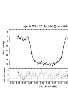
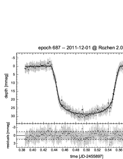
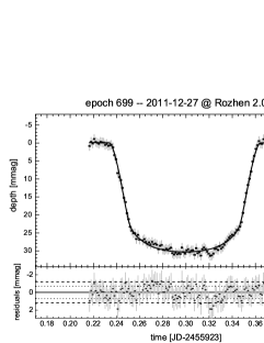
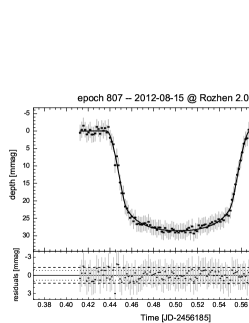
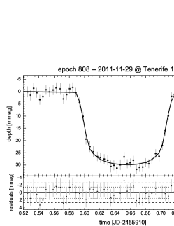
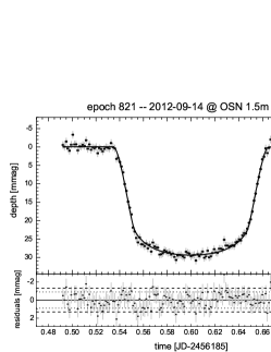
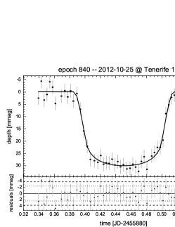
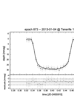
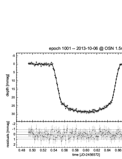
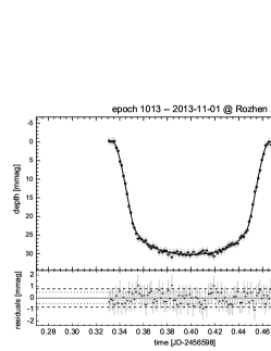
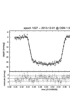
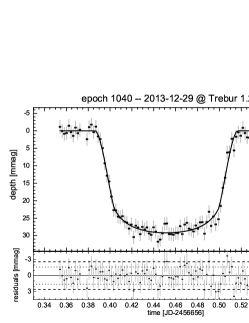
Figure 1: The threefold binned transit light curves of those 18 complete transit event observations, where no simultaneous observations at different telescopes could be achieved. The upper panels show the light curve, the lower panels show the residuals. The rms of the fit in the original (dashed lines) and the threefold binned light curve (dotted lines) are shown as well.

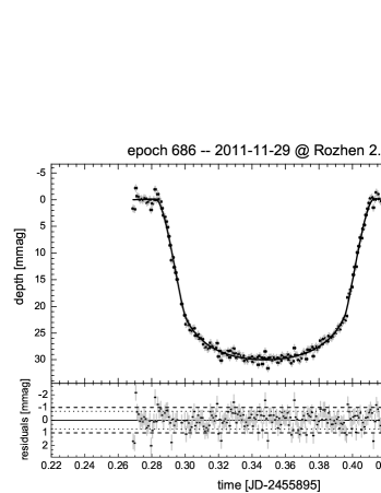
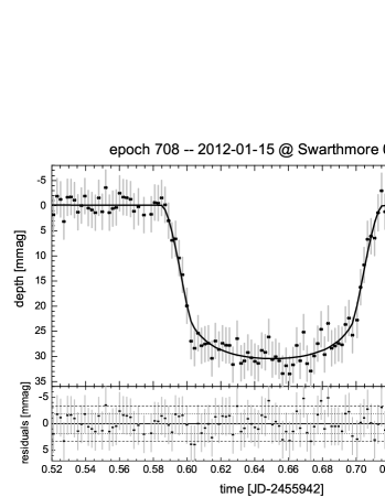
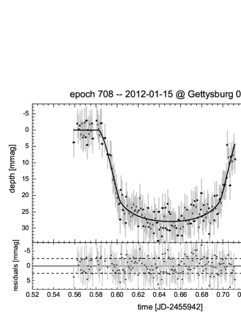
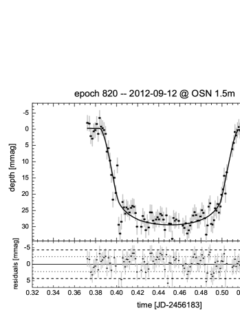
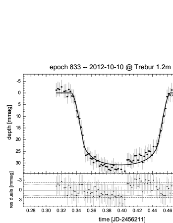
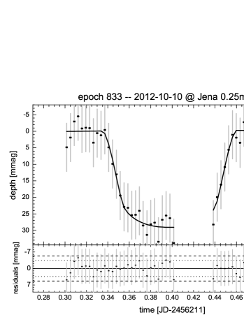
Figure 2: The threefold binned transit light curves of those four transit event observations, where simultaneous observations at two different telescopes could be achieved. The upper panels show the light curve, the lower panels show the residuals. The rms of the fit in the original (dashed lines) and the binned light curve (dotted lines) are shown as well.

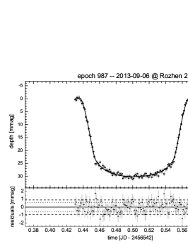
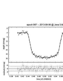
Figure 3: The threefold binned transit light curves of the transit event on 2013 September 6. The transit was observed from three different observatories simultaneously: Rozhen 2.0m, Jena 0.6m, and Torun 0.6m. The upper panels show the light curve, the lower panels show the residuals. The rms of the fit in the original (dashed lines) and the binned light curve (dotted lines) are shown as well.

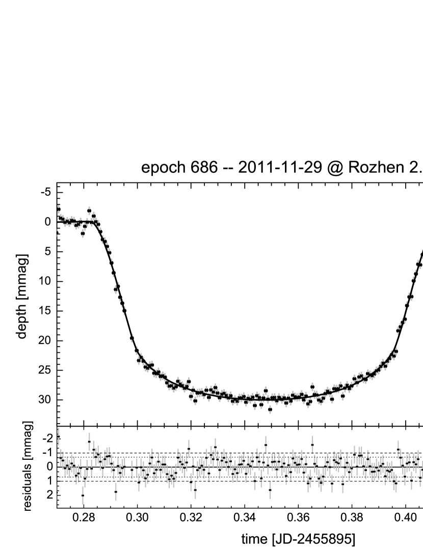
Figure 4: The best transit light curve obtained for this program so far observed with the 2m Rozhen telescope. The rms of the fit is 1.0 and 0.7 mmag in the unbinned and binned light curve, respectively. The mid-transit time has a fitting precision of 14 s.

After fitting an individual transit with both JKTEBOP and TAP there are (typically) eight different fit results (two programs with fixed and free limb-darkening using binned and unbinned data, respectively) with in total 28 individually derived error bars for the properties $i$, $R_{\textrm{p}}/R_{\textrm{s}}$, $T_{\textrm{mid}}$, and $r_{\textrm{p}}+r_{\textrm{s}}$ or $a/R_{\textrm{s}}$.

Regarding all properties, the fit results for the original light curves and the binned ones show no significant differences. Especially concerning the precision of the mid-transit time the results can not be improved by binning the light curve. Though one can reduce the error of an individual data point, one reduces the timing resolution and hence decreases the timing precision (as well as the overall fitting precision; discussed in detail in e.g. Kipping, 2010). Thus, to get one final result for each transit event, we first convert $r_{\textrm{p}}+r_{\textrm{s}}$ to $a/R_{\textrm{s}}$ and then take the average of all obtained values.

In all cases the spread of the fitted values is smaller than the averaged error bar, hence the differences between the models are smaller than the fitting precision. This result is in good agreement with those of e.g. Hoyer, Rojo, & López-Morales (2012). Nevertheless, as previously discussed in e.g. Maciejewski et al. (2013a) and Carter & Winn (2009), JKTEBOP may underestimate the error bars. Though, in this work the differences between the errors derived by JKTEBOP (Monte Carlo, residual-shift, and bootstrapping) and those of TAP (MCMC) are not as noticeable as in e.g. Maciejewski et al. (2013a) (especially for $i$, $R_{\textrm{p}}/R_{\textrm{s}}$, and $a/R_{\textrm{s}}$, but larger for $T_{\textrm{mid}}$), the mean errors derived by the TAP-code are used as final errors.

Keeping the LD coefficients fixed at their theoretical values does not result in significant differences of the light curve fit. This is true for the value as well as the error estimations.

The final light curves and the model fits are shown in Fig. 1 for the single site, and Fig. 2, and 3 for the multi site observations. Our most precise light curve has been obtained using the Rozhen 2.0m telescope and is shown in Fig. 4.

4.1 Transit timing

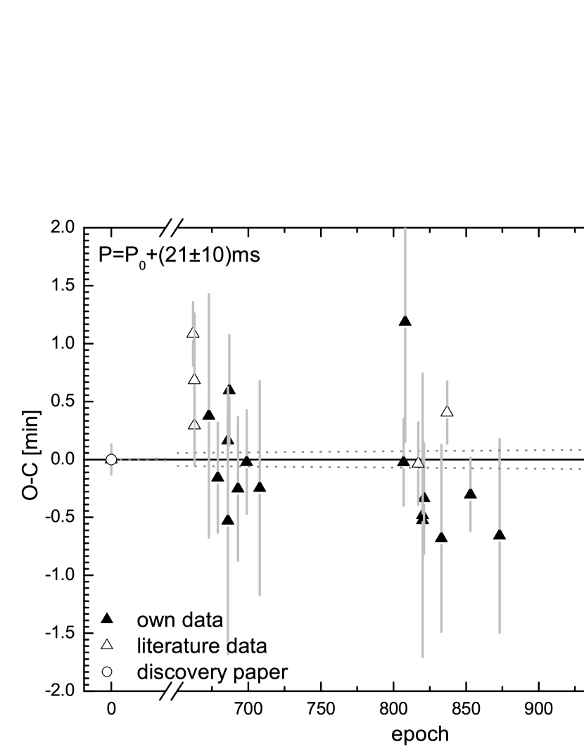
Figure 5: The O–C diagram for HAT-P-32b assuming the circular orbit parameters from Hartman et al. (2011). The open circle denotes literature data from Hartman et al. (2011), open triangles denote data from Sada et al. (2012), and Gibson et al. (2013), the filled triangles denote our data (from Jena, Tenerife, Rozhen, Sierra Nevada, Swarthmore and Trebur). Redetermining the linear ephemeris by $21\>$ms can explain almost all points (black line denotes the fit, black dotted line the fit error), except for some outliers.

The goal of this ongoing project is to look for transit timing variations of known transiting planets where an additional body might be present (see section 1). In case of HAT-P-32b, we have obtained 24 transit light curves with precise mid-transit times out of 45 observations (see Tables 2 and 3). Unfortunately, there are long observational gaps between epochs 720 and 800, and epochs 880 and 980, which is not only due to the non-observability in northern summertime, but also due to the bad weather during the last northern winter affecting most participating YETI telescopes.

After the fitting process, each obtained mid-transit time has to be converted from JD${}_{\textrm{UTC}}$ to barycentric Julian dates in the barycentric dynamical time (BJD${}_{\textrm{TDB}}$) to account for the Earth’s movement. We use the online converter made available by Jason Eastman (see Eastman, Siverd, & Gaudi, 2010) to do the corrections. Since the duration of the transit is just $\sim 3\>$ hours, converting the mid-transit time is sufficient. The different positions of the Earth at the beginning and the end of the transit event is negligible with respect to the overall fitting precision of the mid-transit time, which makes a prior time conversion of the whole light curve unnecessary.

As already mentioned in section 3.1 it is extremely useful for transit timing analysis to have simultaneous observations from different telescopes. Since these data typically are not correlated to each other regarding e.g. the start of observation, observing cadence between two images, field of view (and hence number of comparison stars), one can draw conclusions on the quality of the data and reveal e.g. synchronization errors. In our case we got simultaneous observations at 10 epochs. Unfortunately one of the epoch 673, 693, 807 and 821 observations, and both epoch 834 observations had to be aborted due to the weather conditions or technical problems. The five remaining simultaneous observations, including the threefold observed transit at epoch 987, are consistent within the error bars (see Table 5). Thus, significant systematic errors can be neglected.

Table 5: The results of the transit time fits of the four successful simultaneous transit observations. The transit mid-time in epoch 686, 708, 833, and 987 observations match within the error bars. Epoch 820 observations even match within $3.5\>$s, which is far below the error bars.

epoch	telescope	$T_{\textrm{mid}}-2\,450\,000\>$d		$\Delta T_{\textrm{mid}}\>$[d]
686	Rozhen 2.0m	$5895.35297$ $\>\pm\>$	$0.00016$	0.00049
686	Tenerife 1.2m	$5895.35248$ $\>\pm\>$	$0.00080$
708	Swarthmore 0.6m	$5942.65287$ $\>\pm\>$	$0.00064$	0.00108
708	Gettysburg 0.4m	$5942.65179$ $\>\pm\>$	$0.00113$
820	OSN 1.5m	$6183.45364$ $\>\pm\>$	$0.00085$	0.00003
820	Trebur 1.2m	$6183.45361$ $\>\pm\>$	$0.00049$
833	Trebur 1.2m	$6211.40361$ $\>\pm\>$	$0.00056$	0.00094
833	Jena 0.25m	$6211.40267$ $\>\pm\>$	$0.00214$
987	Rozhen 2.0m	$6542.50530$ $\>\pm\>$	$0.00018$	0.00016
987	Jena 0.6m	$6542.50538$ $\>\pm\>$	$0.00032$
987	Torun 0.6m	$6542.50522$ $\>\pm\>$	$0.00052$

The resultant Observed-minus-Calculated (O–C) diagram is shown in Fig. 5. In addition to our data, the originally published epoch from Hartman et al. (2011), three data points from Sada et al. (2012), and two data points from Gibson et al. (2013) are included. We can explain almost all points by refining the linear ephemeris by $\Delta P=\left(21\pm 10\right)\>$ms. Thus the newly determined period is

$P_{\textrm{new}}$ $\>=\>$	($2.15000825$ $\>\pm\>$	$0.00000012$) d
$P_{\textrm{old}}$ $\>=\>$	($2.150008$ $\>\pm\>$	$0.000001\phantom{00}$) d

From the present O–C diagram- we conservatively can rule out TTV amplitudes larger than $\sim 1.5\>$min. Assuming a circular orbit for both the known planet, and an unseen perturber, we can calculate the minimum perturber mass needed to create that signal. In Fig. 6, all configurations above the solid black line can be ruled out, for they would produce a TTV amplitude larger than $\sim 1.5\>$min. Taking a more restrictive signal amplitude of $\sim 1.0\>$min, all masses above the dotted line can be ruled out. For our calculations we used the n-body integrator Mercury6 (Chambers, 1999) to calculate the TTV signal for 73 different perturber masses between 1 Earth mass and 9 Jupiter masses placed at 1745 different distances to the host star ranging from 0.017 AU to 0.1 AU (i.e. from three times the radius of the host star to three times the semimajor axis of HAT-P-32b). These 127385 different configurations have been analysed to search for those systems that produce a TTV signal of at least $\sim 1.5\>$min and $\sim 1.0\>$min, respectively. In an area around the known planet (i.e. the grey shaded area in Fig. 6 corresponding to $\sim 4$ Hill radii), most configurations were found to be unstable during the simulated time-scales. Within the mean motion resonances, especially the $1:2$ and $2:1$ resonance, only planets with masses up to a few Earth masses can still produce a signal comparable to (or lower than) the spread seen in our data. Such planets would be too small to be found by ground-based observations directly. For distances beyond 0.1 AU, and accordingly beyond a period ratio above 3, even planets with masses up to a few Jupiter masses would be possible. But those planets would generate large, long period transit or radial velocity (RV) signals. Hence one can refuse the existence of such perturbers.

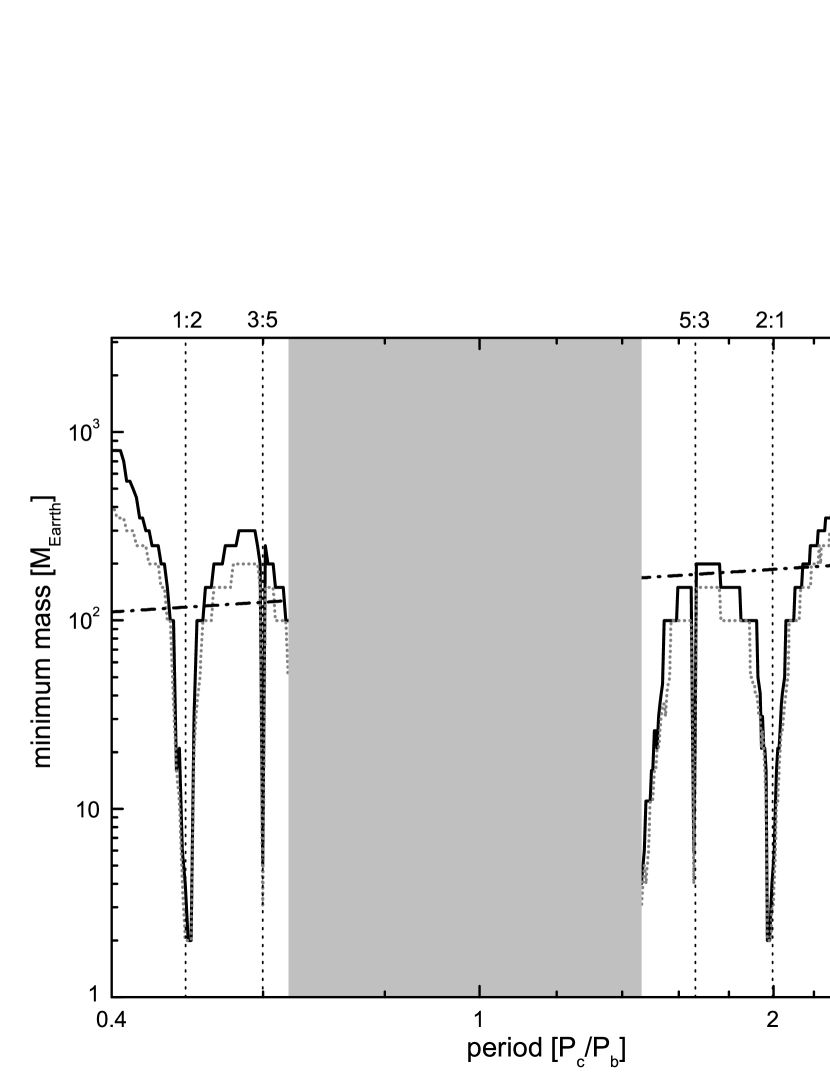
Figure 6: The minimum mass of a perturber needed to create a TTV signal of $\sim 1.5\>$min (solid line) and $\sim 1.0\>$min (dotted line) as a function of the period fraction of the perturber $P_{c}$ and the known planet $P_{b}$. The dash-dotted line indicates the upper mass limit for additional planets assuming them to produce a RV amplitude in the order of the observed RV jitter of $\sim 63.5\>$m/s. Within the mean motion resonances perturbers with less than $2$ Earth masses can not be excluded. The grey shaded area around $P_{c}/P_{b}=1$ denotes the dynamically instable region around the known planet HAT-P-32b corresponding to $\sim 4$ Hill radii.

4.2 Inclination, transit duration and transit depth

The two transit properties duration and depth are directly connected to the physical properties $a/R_{\textrm{s}}$ and $R_{\textrm{p}}/R_{\textrm{s}}$, respectively. Assuming a stable single-planet system, we expect the transit duration to be constant. Even if an exo-moon is present, the resultant variations are in the order of a few seconds (for example calculations see Kipping, 2009) and hence too small to be recognized using ground based observations. Using the obtained fitting errors (as described above) as instrumental weights for a linear fit, we obtain $a/R_{\textrm{s}}=\,$$6.056$ $\,\pm\,$$0.009$ (see Fig. 7). This value confirms the result of Hartman et al. (2011) with $a/R_{\textrm{s}}=6.05\pm 0.04$.

A similar result can be achieved for the transit depth in Fig. 8 represented by the value of $k=R_{\textrm{p}}/R_{\textrm{s}}$. Assuming a constant value, we get a fit result of $k=\,$$0.1510$ $\,\pm\,$$0.0004$ compared to the originally published value of $k=0.1508\pm 0.0004$ by Hartman et al. (2011). Gibson et al. (2013) found an M-dwarf $\approx 2.8^{\prime\prime}$ away from HAT-P-32. Though Knutson et al. (2013) ruled out the possibility that this star is responsible for the long term trend seen in the RV data, due to the size of our apertures this star always contributes to the brightness measurements of the main star and hence can affect the resulting planet-to-star radius ratio. Since actual brightness measurements of the star are not available but needed to correct the influence on the parameters, we do not correct for the M-dwarf. This way, the results are comparable to those of previous authors, but underestimate the true planet-to-star radius ratio. The spread seen in Fig. 8 can therefore be an effect due to the close M-star, or may be also caused by different filter curves of different observatories. Possible filter-dependent effects to the transit depth are discussed in Bernt et al. (2014, in prep.).

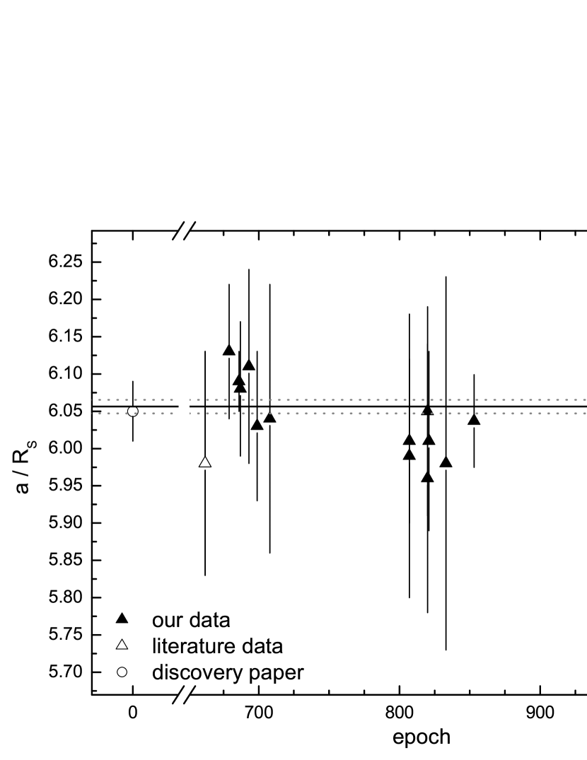
Figure 7: The obtained values for the ratio of the semimajor axis over the stellar radius $a/R_{\textrm{s}}$. Assuming a constant value, the formal best fit using the model fit errors as instrumental weights is found to be $a/R_{\textrm{s}}=\,$$6.056$ $\,\pm\,$$0.009$ (dotted line), which is in agreement with the published value of $a/R_{\textrm{s}}=6.05\pm 0.04$ (Hartman et al., 2011).

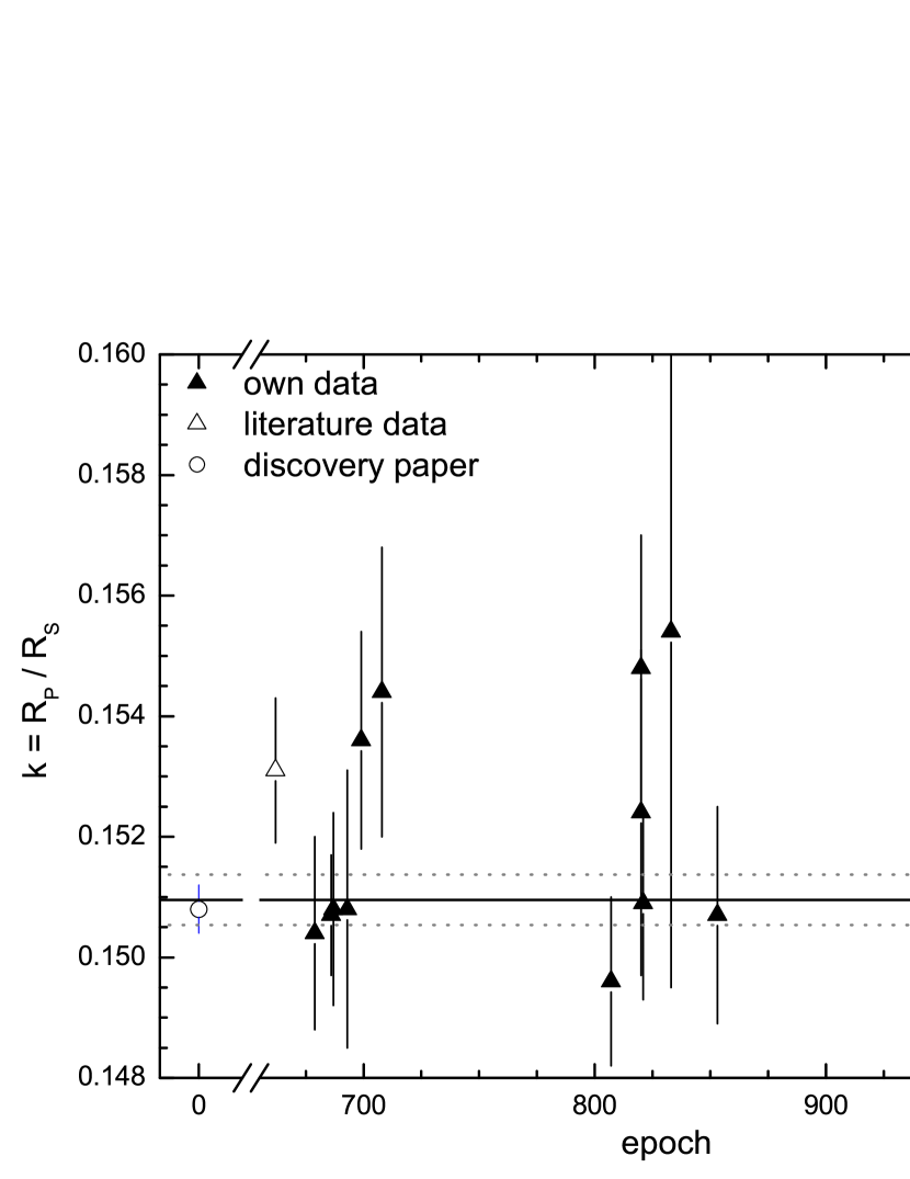
Figure 8: The obtained values for the ratio of the radii $k=R_{\textrm{p}}/R_{\textrm{s}}$. Assuming a constant value, the best fit using the model fit errors as instrumental weights is found to be $k=\,$$0.1510$ $\,\pm\,$$0.0004$ (dotted line), compared to the published value of $k=0.1508\pm 0.0004$ by Hartman et al. (2011).

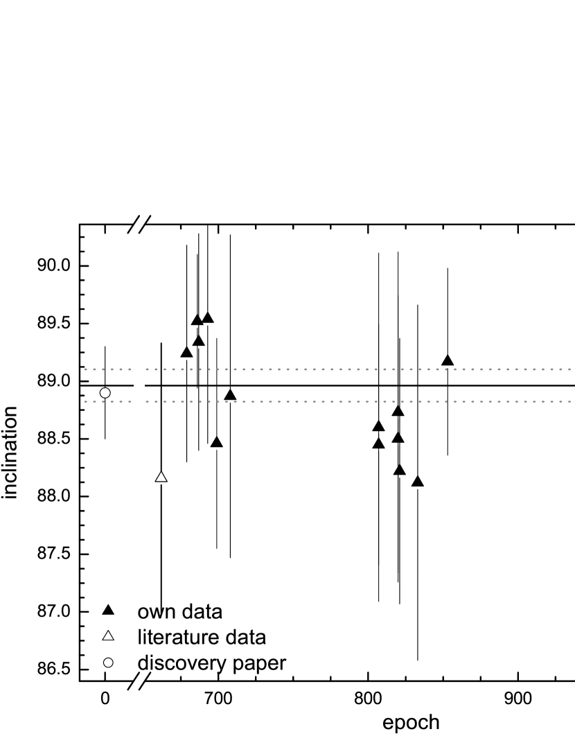
Figure 9: Inclination versus epoch for the HAT-P-32 system. No change in inclination can be seen. The best fit using the model fit errors as instrumental weights is $i=($$88.92$ $\,\pm\,$$0.10$ $)^{\circ}$ (dotted line), compared to $\left(88.9\pm 0.4\right)^{\circ}$ of Hartman et al. (2011)

As expected, also the inclination is found to be consistent with the originally published value. Moreover, due to the number of data points and assuming a constant inclination, we can improve the value to $i=($$88.92$ $\pm$$0.10$ $)^{\circ}$ (see Fig 9). Table 6 summarizes all our results and compares them to the stellar parameters taken from the circular orbit fit of Hartman et al. (2011).

Table 6: A comparison between the results obtained in our analysis, and the literature data from Hartman et al. (2011), Sada et al. (2012), and Gibson et al. (2013). All epochs $T_{0}$ are converted to $BJD_{TDB}$.

	$T_{0}\,[d]$		$P\,[d]$		$a/R_{\textrm{s}}$		$k=R_{\textrm{p}}/R_{\textrm{s}}$		$i\,[^{\circ}]$
our analysis	$2454420.44645$ $\,\pm\,$	$0.00009$	$2.15000825$ $\,\pm\,$	$0.00000012$	$6.056$ $\,\pm\,$	$0.009$	$0.1510$ $\,\pm\,$	$0.0004$	$88.92$ $\,\pm\,$	$0.10$
Hartman et al. (2011)	$2454420.44637$ $\,\pm\,$	$0.00009$	$2.150008$ $\,\pm\,$	$0.000001\>$	$6.05\phantom{0}\,_{-0.04}^{+0.03}$		$0.1508$ $\,\pm\,$	$0.0004$	$88.9$ $\,\pm\,$	$0.4$
Sada et al. (2012)	$2454420.44637$ $\,\pm\,$	$0.00009$	$2.1500103$ $\,\pm\,$	$0.0000003$	$5.98\phantom{0}\,_{-0.10}^{+0.15}$		$0.1531$ $\,\pm\,$	$0.0012$	$86.16\,_{-1.17}^{+1.03}$
Gibson et al. (2013)	$2454942.899220$ $\,\pm\,$	$0.000077$	$2.1500085$ $\,\pm\,$	$0.0000002$	$6.091\,_{-0.036}^{+0.047}$		$0.1515$ $\,\pm\,$	$0.0012$	$89.12\,_{-0.61}^{+0.68}$

4.3 Further limitations

Besides the transit observations, we are also reanalysing the published RV-data (available at Hartman et al., 2011) with the systemic console (Meschiari et al., 2009). It is indeed possible to increase the precision of the RV fit by putting additional, even lower mass or distant bodies into the system. However, due to the large observational gaps seen in Fig. 5, the large number of different possible scenarios, especially perturbers with larger periods, can hardly be restricted. Assuming a small perturber mass, an inclination $\sim 90^{\circ}$, and an eccentricity equal to zero, one can easily derive the expected RV amplitude to be

$$K\simeq\frac{28.4\cdot M_{P}}{P_{c}^{1/3}\cdot M_{s}^{2/3}}$$

using Keplers laws and the conservation of momentum with the perturber mass $M_{P}$ in Jupiter masses, its period $P_{c}$ in days and mass of the central star $M_{S}$ in solar masses. The jitter amplitude of $\sim 63.5\>$m/s found by Knutson et al. (2013) then corresponds to a specific maximum mass of a potentially third body in the system, depending on its period. Hence, all objects above the dash dotted line in Fig. 6 can be ruled out, since they would result in even larger RV amplitudes.

In addition to the advantage of simultaneous observations concerning the reliability on the transit timing, one can also use them as quality markers for deviations in the light curve itself. As seen in Fig. 3, there are no systematic differences between the three light curves obtained simultaneously. This is also true for the data shown in Fig. 2, where no residual pattern is seen twice, though there is a small bump in the epoch 686 Teneriffe data. Hence, one can rule out real astrophysical reasons, e.g. the crossing of a spotty area on the host star, as cause for the brightness change. In a global context, no deviations seen in the residuals of our light curves are expected to be of astrophysical origin.

Folding the residuals of all light curves obtained within this project to a set of trial periods between $0.15\,$d and $2.15\,$d, i.e. period fractions of $P_{c}/P_{b}=\{0.1\ldots 1\}$, we can analyse the resulting phase folded light curves regarding the orbital coverage. Thus, we can check if we would have seen the transit of an inner perturber just by chance while observing transits of HAT-P-32b. Though the duration of a single transit observation is limited to a few hours, taking the large number of observations spread over several months we are still able to cover a large percentage of the trial orbits. As seen in Fig. 10 we achieve an orbital coverage of more than $90\%$ for the majority of trial periods. For a small number of certain periods the coverage drops to $\sim 80\%$. Especially within the resonances it drops to $\sim 60\%$. Assuming the detectability of all transit like signatures with amplitudes more than $3\>$mmag (see residuals in Fig. 1), we can rule out the existence of any inner planet bigger than $\sim 0.5\>$R_jup. Depending on the composition (rocky or gaseous) and bloating status of inner planets, this gives further constraints on the possible perturber mass.

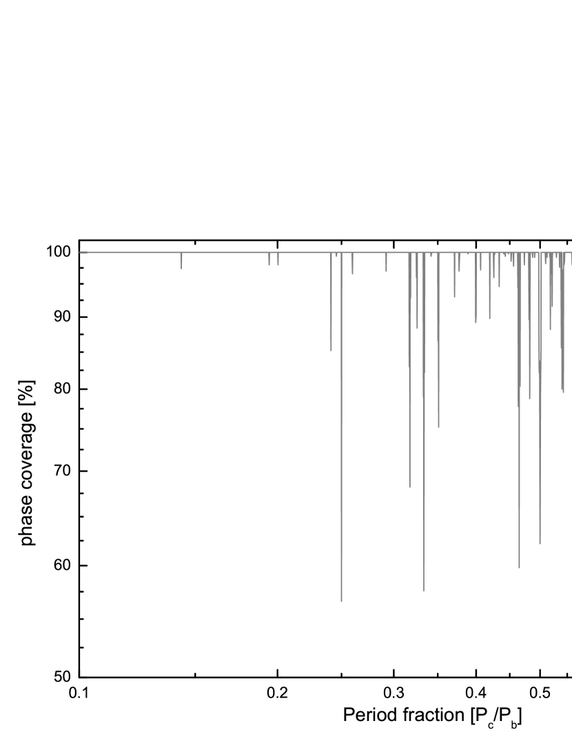
Figure 10: The orbital coverage for an inner transiting perturber as a function of the period fraction of the perturber $P_{c}$ and the known transiting planet $P_{b}$. The unstable area ($\sim 4$ Hill radii) around the known transiting planet is marked in grey.

Finally, it is important to state that all findings assume a perturber on a circular orbit, and with the same inclination as the known planet. It is not unlikely that the inclination of a potential second planet is significantly different from the known transiting planet, as pointed out e.g. by Steffen et al. (2012) and Payne & Ford (2011). This of course also increases the mass needed to create a certain TTV signal. Furthermore, the mass range of planets hidden in the RV jitter is also increased. While a possible eccentric orbit of an inner perturber is limited to a small value due to stability reasons, an outer – not necessarily transiting – perturber on an eccentric orbit is also possible, which in turn also would affect the TTV and RV signal. The companion candidate discovered by Gibson et al. (2013), as well as the proposed originator of the RV long term trend (Knutson et al., 2013) can, however, not be responsible neither for the RV jitter, nor for the still present spread in the O–C diagram.

5 Summary

Table 7: The fit results for the 20 good transit light curves (top rows) as well as the five literature data points from Sada et al. (2012) and Gibson et al. (2013) (middle rows) for the values $T_{\textrm{mid}}$, $a/R_{\textrm{s}}$, $k=R_{\textrm{p}}/R_{\textrm{s}}$ and $i$. Since Sada et al. (2012) did not publish all values for each transit fit, only the transit mid time is tabulated for most observations, except the epoch 662 observation, where also the other parameters are available. The formal $rms$ and the resultant $pnr$ are given in the last column, if available. In the bottom rows the results of the complete observations with larger error bars are given for completeness. In case of the Tenerife 1.2m observations, quasi-simultaneous observations in the filters $r_{p}$ and $B$ have been performed leading to higher $pnr$ values.

date	epoch	telescope	$T_{\textrm{mid}}-2\,450\,000\>$d		$a/R_{\textrm{s}}$		$k=R_{\textrm{p}}/R_{\textrm{s}}$		$i\,[^{\circ}]$		$rms\>$[mmag]	$pnr\>$[mmag]
2011-11-01	673	Tenerife 1.2m	$5867.40301$ $\>\pm\>$	$0.00073$	–		–		–		$2.3$	$3.20$
2011-11-14	679	Jena 0.6m	$5880.30267$ $\>\pm\>$	$0.00033$	$6.13$ $\>\pm\>$	$0.09$	$0.1493$ $\>\pm\>$	$0.0016$	$89.3$ $\>\pm\>$	$1.0$	$1.9$	$1.97$
2011-11-29	686	Rozhen 2.0m	$5895.35297$ $\>\pm\>$	$0.00016$	$6.09$ $\>\pm\>$	$0.04$	$0.1507$ $\>\pm\>$	$0.0010$	$89.5$ $\>\pm\>$	$0.6$	$1.0$	$0.62$
2011-11-29	686	Tenerife 1.2m	$5895.35249$ $\>\pm\>$	$0.00080$	–		–		–		$1.7$	$2.36$
2011-12-01	687	Rozhen 2.0m	$5897.50328$ $\>\pm\>$	$0.00033$	$6.08$ $\>\pm\>$	$0.09$	$0.1508$ $\>\pm\>$	$0.0016$	$89.3$ $\>\pm\>$	$0.9$	$1.5$	$0.94$
2011-12-14	693	Rozhen 0.6m	$5910.40274$ $\>\pm\>$	$0.00043$	$6.11$ $\>\pm\>$	$0.13$	$0.1508$ $\>\pm\>$	$0.0023$	$89.5$ $\>\pm\>$	$1.1$	$2.0$	$3.40$
2011-12-27	699	Rozhen 2.0m	$5923.30295$ $\>\pm\>$	$0.00031$	$6.03$ $\>\pm\>$	$0.10$	$0.1536$ $\>\pm\>$	$0.0018$	$88.5$ $\>\pm\>$	$0.9$	$1.2$	$0.96$
2012-01-15	708	Swarthmore 0.6m	$5942.65287$ $\>\pm\>$	$0.00064$	$6.04$ $\>\pm\>$	$0.18$	$0.1544$ $\>\pm\>$	$0.0024$	$88.9$ $\>\pm\>$	$1.4$	$3.3$	$3.28$
2012-08-15	807	Rozhen 2.0m	$6155.50385$ $\>\pm\>$	$0.00026$	$6.01$ $\>\pm\>$	$0.11$	$0.1496$ $\>\pm\>$	$0.0014$	$88.5$ $\>\pm\>$	$1.0$	$1.3$	$1.11$
2012-08-18	808	Tenerife 1.2m	$6157.65470$ $\>\pm\>$	$0.00072$	–		–		–		$2.6$	$3.71$
2012-09-12	820	OSN 1.5m	$6183.45364$ $\>\pm\>$	$0.00085$	$5.96$ $\>\pm\>$	$0.18$	$0.1524$ $\>\pm\>$	$0.0027$	$88.7$ $\>\pm\>$	$1.4$	$4.3$	$4.85$
2012-09-12	820	Trebur 1.2m	$6183.45361$ $\>\pm\>$	$0.00049$	$6.05$ $\>\pm\>$	$0.14$	$0.1548$ $\>\pm\>$	$0.0022$	$88.5$ $\>\pm\>$	$1.2$	$2.1$	$2.33$
2012-09-14	821	OSN 1.5m	$6185.60375$ $\>\pm\>$	$0.00033$	$6.01$ $\>\pm\>$	$0.12$	$0.1509$ $\>\pm\>$	$0.0016$	$88.2$ $\>\pm\>$	$1.2$	$1.3$	$1.07$
2012-10-10	833	Trebur 1.2m	$6211.40361$ $\>\pm\>$	$0.00056$	$5.98$ $\>\pm\>$	$0.25$	$0.1554$ $\>\pm\>$	$0.0059$	$88.1$ $\>\pm\>$	$1.5$	$2.2$	$2.18$
2012-11-22	853	OSN 1.5m	$6254.40404$ $\>\pm\>$	$0.00022$	$6.037$ $\>\pm\>$	$0.062$	$0.1507$ $\>\pm\>$	$0.0018$	$89.2$ $\>\pm\>$	$0.8$	$1.1$	$0.84$
2013-01-04	873	Tenerife 1.2m	$6542.40397$ $\>\pm\>$	$0.00058$	–		–		–		$1.9$	$2.87$
2013-09-07	987	Jena 0.6m	$6542.50538$ $\>\pm\>$	$0.00032$	$6.04$ $\>\pm\>$	$0.11$	$0.1497$ $\>\pm\>$	$0.0016$	$88.7$ $\>\pm\>$	$1.1$	$1.6$	$1.57$
2013-09-07	987	Rozhen 2.0m	$6542.50530$ $\>\pm\>$	$0.00018$	$5.97$ $\>\pm\>$	$0.09$	$0.1535$ $\>\pm\>$	$0.0012$	$88.3$ $\>\pm\>$	$0.8$	$0.9$	$0.67$
2013-09-07	987	Torun 0.6m	$6542.50522$ $\>\pm\>$	$0.00052$	$5.89$ $\>\pm\>$	$0.20$	$0.1515$ $\>\pm\>$	$0.0029$	$87.9$ $\>\pm\>$	$1.4$	$3.5$	$2.33$
2013-10-06	1001	OSN 1.5m	$6572.60532$ $\>\pm\>$	$0.00018$	$6.11$ $\>\pm\>$	$0.06$	$0.1465$ $\>\pm\>$	$0.0013$	$89.2$ $\>\pm\>$	$0.7$	$0.9$	$0.63$
2013-11-01	1013	Rozhen 2.0m	$6598.40539$ $\>\pm\>$	$0.00017$	$6.05$ $\>\pm\>$	$0.06$	$0.1511$ $\>\pm\>$	$0.0010$	$88.9$ $\>\pm\>$	$0.8$	$0.8$	$0.68$
2013-11-03	1014	OSN 1.5m	$6600.55546$ $\>\pm\>$	$0.00017$	$6.02$ $\>\pm\>$	$0.05$	$0.1503$ $\>\pm\>$	$0.0009$	$89.2$ $\>\pm\>$	$0.8$	$1.3$	$1.33$
2013-12-01	1027	OSN 1.5m	$6628.50585$ $\>\pm\>$	$0.00031$	$6.13$ $\>\pm\>$	$0.09$	$0.1475$ $\>\pm\>$	$0.0022$	$89.2$ $\>\pm\>$	$0.9$	$1.8$	$1.59$
2013-12-29	1040	Trebur 1.2m	$6656.45533$ $\>\pm\>$	$0.00045$	$6.07$ $\>\pm\>$	$0.13$	$0.1509$ $\>\pm\>$	$0.0022$	$88.8$ $\>\pm\>$	$1.1$	$2.6$	$2.74$
2011-10-09	662	KPNO 2.1m	$5843.75341$ $\>\pm\>$	$0.00019$	$5.98\phantom{0\>}_{-\>0.15}^{+\>0.10}$		$0.1531$ $\>\pm\>$	$0.0012$	$88.2\>_{-\>1.0}^{+\>1.2}$		–	–
2011-10-11	663	KPNO 2.1m	$5845.90287$ $\>\pm\>$	$0.00024$	–		–		–		–	–
2011-10-11	663	KPNO 0.5m	$5845.90314$ $\>\pm\>$	$0.00040$	–		–		–		–	–
2012-09-06	817	Gibson et al. (2013)	$6177.00392$ $\>\pm\>$	$0.00025$	–		–		–		–	–
2012-10-19	837	Gibson et al. (2013)	$6220.00440$ $\>\pm\>$	$0.00019$	–		–		–		–	–
2011-10-04	660	Ankara 0.4m	$5839.45347$ $\>\pm\>$	$0.00101$	$5.9$ $\>\pm\>$	$0.2$	$0.1448$ $\>\pm\>$	$0.0021$	$88.1$ $\>\pm\>$	$1.4$	$4.7$	$2.22$
2012-01-15	708	Gettysburg 0.4m	$5942.65179$ $\>\pm\>$	$0.00113$	$5.79$ $\>\pm\>$	$0.36$	$0.1493$ $\>\pm\>$	$0.0054$	$87.3$ $\>\pm\>$	$1.7$	$2.5$	$4.25$
2012-10-10	833	Jena 0.25m	$6211.40267$ $\>\pm\>$	$0.00214$	$6.04$ $\>\pm\>$	$0.65$	$0.1514$ $\>\pm\>$	$0.0089$	$86.5$ $\>\pm\>$	$2.5$	$5.3$	$6.96$
2012-10-25	840	Tenerife 1.2m	$6226.45618$ $\>\pm\>$	$0.00102$	–		–		–		$3.8$	$5.05$
2012-12-22	867	Tenerife 1.2m	$6284.50460$ $\>\pm\>$	$0.00100$	–		–		–		$3.3$	$5.10$

We presented our observations of HAT-P-32b planetary transits obtained during a timespan of 24 months (2011 October until 2013 October). The data were collected using telescopes all over the world, mainly throughout the YETI network. Out of 44 started observations we obtained 24 light curves that could be used for further analysis. 21 light curves have been obtained that could not be used due to different reasons, mostly bad weather. In addition to our data, literature data from Hartman et al. (2011), Sada et al. (2012), and Gibson et al. (2013) were also taken into account (see Fig. 5, 7, 8, and 9 and Table 7).

The published system parameters $a/R_{\textrm{s}}$, $R_{\textrm{p}}/R_{\textrm{s}}$ and $i$ from the circular orbit fit of Hartman et al. (2011) were confirmed. In case of the semimajor axis over the stellar radius and the inclination, we were able to improve the results due to the number of observations. As for the planet-to-star radius ratio, we did not achieve a better solution for there is a spread in the data making constant fits difficult. In addition, Gibson et al. (2013) found an M-dwarf $\approx 2.8^{\prime\prime}$ away from HAT-P-32 and hence a possible cause for this spread.

Regarding the transit timing, a redetermination of the planetary ephemeris by $21\>$ms can explain the obtained mid-transit times, although there are still some outliers. Of course, having 1$\sigma$ error bars, one would expect some of the data points to be off the fit. Nevertheless, due to the spread of data seen in the O–C diagram, observations are planned to further monitor HAT-P-32b transits using the YETI network. This spread in the order of $\sim 1.5\>$min does not exclude certain system configurations. Assuming circular orbits even an Earth mass perturber in a mean motion resonance could still produce such a signal.

References

- Bakos et al. (2009) Bakos G. Á., et al., 2009, ApJ, 707, 446
- Broeg et al. (2005) Broeg C., Fernández M., Neuhäuser R., 2005, AN, 326, 134
- Carter & Winn (2009) Carter J. A., Winn J. N., 2009, ApJ, 704, 51
- Carter & Winn (2010) Carter J. A., Winn J. N., 2010, ApJ, 716, 850
- Chambers (1999) Chambers J. E., 1999, MNRAS, 304, 793
- Claret (2000) Claret 2000, A&A 363, 1081
- Eastman et al. (2013) Eastman J., Gaudi B. S., Agol E., 2013, PASP, 125, 83
- Eastman et al. (2010) Eastman J., Siverd R., Gaudi B. S., 2010, PASP, 122, 935
- Etzel (1981) Etzel P. B., 1981, psbs.conf, 111
- Fulton et al. (2011) Fulton B. J., Shporer A., Winn J. N., Holman M. J., Pál A., Gazak J. Z., 2011, AJ, 142, 84
- Gazak et al. (2012) Gazak J. Z., Johnson J. A., Tonry J., Dragomir D., Eastman J., Mann A. W., Agol E., 2012, AdAst, 2012, 30
- Gibson et al. (2013) Gibson N. P., Aigrain S., Barstow J. K., Evans T. M., Fletcher L. N., Irwin P. G. J., 2013, arXiv, arXiv:1309.6998
- Hartman et al. (2011) Hartman J. D., et al., 2011, ApJ, 742, 59
- Hoyer et al. (2012) Hoyer S., Rojo P., López-Morales M., 2012, ApJ, 748, 22
- Kipping (2009) Kipping D. M., 2009, MNRAS, 392, 181
- Kipping (2010) Kipping D. M., 2010, MNRAS, 408, 1758
- Knutson et al. (2013) Knutson H. A., et al., 2013, arXiv, arXiv:1312.2954
- Lloyd et al. (2013) Lloyd J. P., et al., 2013, arXiv, arXiv:1309.1520
- Maciejewski et al. (2010) Maciejewski G., et al., 2010, MNRAS, 407, 2625
- Maciejewski et al. (2011a) Maciejewski G., Errmann R., Raetz S., Seeliger M., Spaleniak I., Neuhäuser R., 2011, A&A, 528, A65
- Maciejewski et al. (2011b) Maciejewski G., et al., 2011, MNRAS, 411, 1204
- Maciejewski et al. (2011c) Maciejewski G., et al., 2011, A&A, 535, 7
- Maciejewski et al. (2013a) Maciejewski G., et al., 2013a, A&A, 551, A108
- Maciejewski et al. (2013b) Maciejewski G., et al., 2013b, AJ, 146, 147
- Mandel & Agol (2002) Mandel K., Agol E., 2002, ApJ, 580, L171
- Meschiari et al. (2009) Meschiari S., Wolf A. S., Rivera E., Laughlin G., Vogt S., Butler P., 2009, PASP, 121, 1016
- Mugrauer & Berthold (2010) Mugrauer M., Berthold T., 2010, AN, 331, 449
- Neuhäuser et al. (2011) Neuhäuser R., et al., 2011, AN, 332, 547
- Nesvorný & Morbidelli (2008) Nesvorný D., Morbidelli A., 2008, ApJ, 688, 636
- Payne & Ford (2011) Payne M. J., Ford E. B., 2011, ApJ, 729, 98
- Pickles & Depagne (2010) Pickles A., Depagne É., 2010, PASP, 122, 1437
- Popper & Etzel (1981) Popper D. M., Etzel P. B., 1981, AJ, 86, 102
- Raetz (2012) Raetz St., 2012, PhD thesis University Jena
- Sada et al. (2012) Sada P. V., et al., 2012, PASP, 124, 212
- Salaris, Chieffi, & Straniero (1993) Salaris M., Chieffi A., Straniero O., 1993, ApJ, 414, 580
- Southworth et al. (2009) Southworth J., et al., 2009, MNRAS, 396, 1023
- Southworth (2008) Southworth J., 2008, MNRAS, 386, 1644
- Steffen et al. (2012) Steffen J. H., et al., 2012, PNAS, 109, 7982
- Szabó et al. (2013) Szabó R., Szabó G. M., Dálya G., Simon A. E., Hodosán G., Kiss L. L., 2013, A&A, 553, A17
- von Essen et al. (2013) von Essen C., Schröter S., Agol E., Schmitt J. H. M. M., 2013, A&A, 555, A92
- Weber et al. (2012) Weber M., Granzer T., Strassmeier K. G., 2012, SPIE, 8451,