Global and Local Information in Clustering Labeled Block Models

Abstract

The stochastic block model is a classical cluster-exhibiting random graph model that has been widely studied in statistics, physics and computer science. In its simplest form, the model is a random graph with two equal-sized clusters, with intra-cluster edge probability $p$, and inter-cluster edge probability $q$. We focus on the sparse case, i.e., $p,q=O(1/n)$, which is practically more relevant and also mathematically more challenging. A conjecture of Decelle, Krzakala, Moore and Zdeborová, based on ideas from statistical physics, predicted a specific threshold for clustering. The negative direction of the conjecture was proved by Mossel, Neeman and Sly (2012), and more recently the positive direction was proven independently by Massoulié and Mossel, Neeman, and Sly.

In many real network clustering problems, nodes contain information as well. We study the interplay between node and network information in clustering by studying a labeled block model, where in addition to the edge information, the true cluster labels of a small fraction of the nodes are revealed. In the case of two clusters, we show that below the threshold, a small amount of node information does not affect recovery. On the other hand, we show that for any small amount of information efficient local clustering is achievable as long as the number of clusters is sufficiently large (as a function of the amount of revealed information).

1 Introduction

The stochastic block model is one of the most popular models for networks with clusters. The model has been extensively studied in statistics [15, 28, 5], computer science (where it is called the planted partition problem) [11, 16, 8, 20] and theoretical statistical physics [9, 30, 10].

The simplest block model has $k$ clusters of equal size, and is generated as follows. Starting with $n$ nodes, each node $v$ is randomly assigned a label $\sigma_{v}$ from the set $\{1,\ldots,k\}$. For each pair of nodes, $(u,v)$, if their labels are identical an edge is added between them with probability $p$, otherwise an edge is added with probability $q$. Often the case when $p>q$ is considered, and the question of interest is understanding how large $p-q$ must be for correct clusters recovery to be possible. In the recovery problem the input consists of the unlabeled graph and the desired output is a partition of the graph.

Real world networks are typically sparse. Thus, an interesting setting in the block model is when $p$ and $q$ are in $O(1/n)$. Here, it is more convenient to parametrize the problem by setting $p=a/n$ and $q=b/n$, where $a,b$ are constants. In the sparse setting, exact recovery is impossible as the resulting graph will have isolated nodes. Moreover, it is easy to see that even nodes with constant degree cannot be classified accurately given all other nodes in the graph. Thus the goal is to find a partition that has non-trivial correlation with the original clusters (up to permutation of cluster labels). This has sometimes been referred to as the cluster detection problem (see e.g. [9]); throughout the paper we refer to it as the cluster recovery problem (though note that the goal is not to recover every cluster with probability 1).

General results of Coja-Oghlan [7] imply that it is possible to identify a partition that is correlated with the true hidden partition when $(a-b)^{2}\geq Ck^{4}(a+(k-1)b)$. A beautiful physics paper by Decelle et al. [9] conjectured that the recovery problem is feasible for the case of two clusters when $(a-b)^{2}>2(a+b)$ and impossible when $(a-b)^{2}<2(a+b)$. The non-reconstructability in the case where $(a-b)^{2}<2(a+b)$ was proved by Mossel, Neeman and Sly [23], and more recently the same authors [25] and Massoulié [19] independently showed that recovery is possible when $(a-b)^{2}>2(a+b)$.

1.1 The labeled stochastic block model

The aforementioned results along with previous results for denser block models provide a detailed picture of recovery in the stochastic block model. However, the model they consider is idealized and does not capture many aspects of real network problems. One such aspect is that in many realistic settings, node label information is available for some of the nodes. For example, in social networks, the group label of some individuals (nodes) is known. In metabolic networks, the function of some of the nodes may be known. Indeed, there has been much recent work in the machine learning and applied networks communities on combining node and network information (see for example [6, 3, 4]). There are several ways in which node and edge information can be incorporated; in real applications nodes and edges contain rich information which is noisy, but correlated with the node’s “true” label and with the “similarity” of pairs of nodes.

In this paper, we study a simple model which incorporates both node and edge information which we call the labeled stochastic block model. This model has been considered previously in the physics literature [9, 29, 1]. In addition to having the unlabeled graph as an input, a small random fraction of the nodes’ labels are also provided as input to the clustering algorithm.

1.2 The big effect of a small number of node labels

It is easy to see that even a vanishing fraction of node labels can play a major role in the cluster recovery problem. For example, consider the denser case where the clusters $C_{1},\ldots,C_{k}$ can be identified accurately [20]. Here, it is impossible to distinguish between a clustering $C_{1},\ldots,C_{k}$ where the nodes in cluster $C_{i}$ have label $i$ and the same clustering where the nodes in cluster $i$ have label $\pi(i)$ for any permutation $\pi$ of the labels. However, note that for any $p>0$, given a $p$-fraction of the node labels, it is possible to identify the permutation $\pi$ correctly with high probability. It is natural to ask if the same result holds in the sparse case, and it is not hard to see that a similar statement can be made (see Proposition 1).

The above observation shows that even a small amount of node information can overcome the problems of symmetry in the stochastic block model. Another problem of symmetry present in the unlabeled model is that there is no local algorithm that can identify clusters better than random guessing. Informally, a local algorithm determines the label of a node based solely on an $o(\log n)$ neighborhood of that node, including possibly uniform independent random variables attached to each node of the graph (see A.2 for a formal definition and  [18, 14] for examples). The proof that a local algorithm cannot detect better than random guessing in this case is folklore, and we include it here for completeness. This limitation in detection may be compared to the problem of finding independent sets, where local algorithms can have non-trivial power (while still being less powerful than global algorithms) [13]. It is therefore natural to ask:

Question 1.

Does a vanishing fraction of labeled nodes allow local algorithms to detect clusters? If so, when?

An even a more direct question relates to the statistical power of revealing some of the node labels. While it is clear that revealing a large fraction of the node labels allows non-trivial recovery, it is far from clear what the effect is when this fraction is vanishingly small. On the one hand, we might expect by continuity that revealing a vanishing fraction of the node labels will be identical in the limit to revealing no labels. On the other hand, we might imagine how a small fraction of the node labels could be used as seeds for recovery algorithms. We thus ask:

Question 2.

Does revealing a vanishing fraction of the node labels change the detectability threshold? Does it change the fraction of correctly labeled nodes?

The latter question was considered in recent work in statistical physics [31, 29, 1].

1.3 Our results

To set the stage for our contributions, we begin with some observations regarding the utility of local information. The proofs of these propositions are straightforward (see Appendix A), but they are useful for establishing context of how information about (a small fraction of) node labels may help. The first is that even a vanishingly small proportion of node labels aids in breaking the symmetry and assigning labels to the cluster assignments.

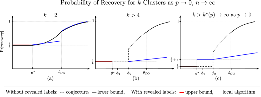
Figure 1: Previous work (black) and our contributions (colored). The $x$-axes represent the second eigenvalue of the corresponding broadcast process on the coupled Galton-Watson Tree when the average degree is fixed–in simpler terms, this is an increasing function of the ratio $\tfrac{a-b}{a}$. In all three cases, $\theta^{*}$ is the reconstruction threshold corresponding to the root reconstruction problem on trees, and $\theta_{CO}$ is the threshold of [7]. In the two-cluster case (Subfigure (a)), $\theta^{*}$ corresponds exactly to the Kesten-Stigum bound of $(a-b)^{2}<2(a+b)$ [9, 23]. For the case of larger $k$, $\theta^{*}<(a-b)^{2}/k(a+(k-1)b)$ (see Subfigures (b), (c) and Proposition 6). We prove analogously that recovery is not possible below $\theta^{*}$ in the labeled model as $p\to 0$ for all $k$ (Theorem 2). In the two-cluster case, recent results of [25] and [19] show that recovery is possible in the range $(\theta^{*},\theta_{CO})$; above $\theta_{CO}$, a combination of the results of [7] and [24] give optimal recovery in the standard model for $k=2$; we observe that in the labeled model for $k=2$, one can reconstruct better than randomly in the range ($\theta^{*}$, $\theta_{CO}$) and optimally above $\theta_{CO}$ using local algorithms (see Propositions 4 and 3). The results of [7] also give non-trivial recovery guarantees above $\theta_{CO}$ for all $k$. In the $k$-cluster case (Figures (b), (c)), the picture is more complicated: $\phi_{1}$ and $\phi_{2}$ are conjectured brute-force and efficient solvability thresholds respectively, both conjectured by [9]—above $\phi_{1}$ recovery is possible via brute-force enumeration, and above $\phi_{2}$ an efficient algorithm for recovery exists. Above $\phi_{2}$, Proposition 4 shows that recovery is possible for $k$ clusters via a local algorithm. In Subfigure (c), for any $b,p$, if $k>k^{*}(p)$ and $(a-b)/k>1$, as in Theorem 1, we give an efficient local recovery algorithm that correctly labels $\frac{1}{k}+\epsilon$ of the nodes, even below the conjectured efficient recovery threshold $\phi_{2}$.

Proposition 1 (Informal version).

Given a clustering algorithm which outputs clusters correlated with the true clustering, a small fraction of revealed node labels is sufficient to output a labeling which is correlated with the true labeling.

In the absence of any node information, it is an easy folklore result that any local algorithm cannot recover clusters. However, we show that in the case of two clusters, when a small fraction of node labels are revealed, a local algorithm is able to recover the clusters optimally. This latter result is a direct corollary of a robust reconstruction result on trees of [24].

Proposition 2 (Informal version).

In the unlabeled stochastic block model, no local algorithm can find a clustering correlated with the true clustering.

Proposition 3 (Informal version).

In an instance of the labeled stochastic block model, when $k=2$, if $(a-b)^{2}>C(a+b)$ for some large constant $C$, then there is a local algorithm which given a vanishing fraction of labeled nodes, reconstruct the label of all nodes with the same accuracy as the optimal (non-local) algorithm for the unlabeled problem.

We also observe that results on census reconstruction [26] imply that above the Kesten-Stigum bound a vanishingly small fraction of revealed nodes suffices for the cluster recovery problem.

Proposition 4 (Informal version).

For any fixed $k$, above the robust reconstruction threshold (i.e. when $(a-b)^{2}>k(a+(k-1)b)$), when the fraction of revealed node labels is vanishingly small, the cluster recovery problem is solvable by a local algorithm.

The proof follows more or less directly from previous results, but we include it in Appendix A.4 for completeness.

In this context, one might expect that labels could allow clustering in the labeled model in regimes which cannot be effectively clustered in the unlabeled model. The case of two clusters is the case we understand the best. Here, utilizing results for the reconstruction problem on trees and of [23], we answer Question 2 in the negative (Theorem 2) and at the same time answer Question 1 positively (Propositions 3 and 4). The complete picture for the case of two clusters is presented in Figure 1(a).

For any fixed $k>2$, the picture is much more complicated. In this case, we observe that below the tree reconstruction threshold (this corresponds to $\theta^{*}$ in Figure 1(b)), a vanishing fraction of node labels do not assist in the cluster recovery problem (see Theorem 2).

Theorem 2 (Informal version).

For any fixed $k$, below the associated tree reconstruction threshold (to be defined later), when the fraction of revealed node labels is vanishingly small, the cluster recovery problem is not solvable. In particular, when $k=2$, the threshold is the Kesten-Stigum bound of $(a-b)^{2}<2(a+b)$; for $k\geq 2$, if $a-b<k$ then recovery is impossible.

Our main interest is in the case when the number of clusters is very large. Here, we consider the setting when the fraction of revealed nodes $p\to 0$, and simultaneously the number of clusters $k=k(p)\rightarrow\infty$. In this setting, we show that revealing node labels has a dramatic effect on the threshold for cluster recovery. We show that a local algorithm successfully solves the cluster recovery problem even below the conjectured algorithmic threshold in the unlabeled case, $(a-b)^{2}=k(a+(k-1)b)$. As the number of clusters $k\to\infty$, our algorithm works all the way down to the tree reconstruction threshold of $(a-b)/k>1$. Moreover, it is impossible to recover (locally or globally) with a vanishing fraction of labeled nodes if $(a-b)/k<1$. Both results follow from the corresponding results on trees.

Theorem 1 (Informal version).

For every $\delta>0$, there exists $\epsilon=\epsilon(\delta)>0$ such that for every $p>0$, if $k=k(p)$ is large enough as a function of $p$ and $a-b>(1+\delta)k$, then the label of a random node can be recovered with probability at least $\tfrac{1}{k}+\epsilon$.

Note that $\epsilon$ depends on $\delta$ but is independent of $p$.

Recent work in statistical physics [31] argues that for every fixed number of clusters $k$, a vanishing fraction of labels does not provide any advantage in the detection probability over having no labels at all. We note that in our results, the order of limits is exchanged as the number of clusters $k$ needed for our results to hold, depends on the fraction of nodes revealed. Thus, there is no contradiction between the results (see also [1, 29]). Figure 1(c) provides a detailed picture of the case in which the number of clusters is very large (in the setting of Theorem 1).

Open Problems

In the case of two clusters, we conjecture that whenever any fraction of node labels are revealed, there is a local algorithm that recovers the clusters optimally. This would follow from a related conjecture regarding information flow on trees stated below. We report some simulations suggesting the veracity of the conjecture in Appendix B.

Conjecture 1 (Informal version).

Let $T$ be an infinite tree with root $\rho$. The tree is labeled from the set $\{\pm 1\}$ as follows. First, the root is assigned a label from $\{\pm 1\}$ at random. Along each edge the label is propagated with probability $1-\eta$ and flipped with probability $\eta$. Let $(T,\tau)$ denote the resulting labeled tree. Add each node independently to a set $R$ with probability $p$. Finally for any $r$, let $\partial T_{r}$ denote the set of leaves at depth $r$. Then, for any value of $p>0$ and $\eta<1/2$,

$$\lim_{r\to\infty}\mathbb{E}\big{|}\Pr[\tau_{\rho}=1~{}|~{}\tau_{R}]-\Pr[\tau_{\rho}=1~{}|~{}\tau_{R},\tau_{\partial T_{r}}]\big{|}=0$$

In addition to Conjecture 1, several interesting questions remain, particularly in the regime where $k$ is large. When $k$ is large, is it possible to use global and local information together to obtain better recovery guarantees? Which algorithmic tools might allow one to use global and local information simultaneously?

Another open problem relates to different types noise models. The assumption in the current paper is that each label is revealed accurately with a vanishing probability. But one may consider other types of noise. In particular, we may assume for example that for each node independently we are given the correct label with small probability $\delta$ and otherwise a uniformly chosen label. Is it true that the same results hold for this noise model as for the noise model considered here? For most of the results presented here, it is easy to see that the answer is yes. However, for one of our main results, Theorem 1, the proof does not extend to the latter noise model. It is an interesting open problem to determine the effect of the noisy information in this setup.

Remark 1.

A short abstract describing these results will appear in proceedings of RANDOM 2014.

Acknowledgments

E.M. thanks Cris Moore, Joe Neeman, Allan Sly and Lenka Zdeborová for many interesting discussions related to the block model. We would like to thank the authors of  [31] for discussion of their work at its early stages. The authors would like to thank the Simons Institute for the Theory of Computing where much of the work reported here was carried out. The authors would also like to thank anonymous referees for their helpful comments.

2 Model

2.1 Stochastic Block Model

The stochastic block model is a generative model for modular random networks, defined by the following set of parameters: the number of clusters $k$, the expected fraction of nodes in each cluster $i$, $\langle f_{i}\rangle_{i=1}^{k}$ , and a $k\times k$ symmetric affinity matrix $P_{i,j}$ indicating the edge probability between nodes of type $i$ and $j$. A random network $G$ on $n$ nodes is generated as follows:

1. First, each node $v$ is assigned a label $\sigma_{v}\in\{1,\ldots,k\}$, s.t. $\Pr[\sigma_{v}=i]=f_{i}$.

2. For every pair of nodes $u,v$, an edge is added between them with probability $P_{\sigma_{u},\sigma_{v}}$, independently for each pair.

In this work, we are mainly interested in the sparse case, i.e., when the average degree of the graph is constant. We focus on the setting where edge probabilities only depend on whether the labels of the endpoint are same or different. Thus, $P_{ii}=a/n$ for $1\leq i\leq k$ and $P_{ij}=b/n$ for $i\neq j$, for constants $a>b$. Also, we focus on the case where $f_{i}=1/k$ for each $i$, i.e., each cluster is roughly of the same size. The model is denoted by ${\mathcal{G}}(n,k,a,b)$, and $(G,\sigma)\sim{\mathcal{G}}(n,k,a,b)$ denotes an instance of a graph generated according to the model, where $\sigma$ are the cluster labels of the nodes.

Labeled Block Model: The labeled block model has an additional parameter $p$, which is the probability with which the true cluster label of any given node is revealed. Thus, if $(G,\sigma)\sim{\mathcal{G}}(n,k,a,b)$ is an instance of the block model, $R\subseteq[n]$ is chosen by placing each node of $G$ in $R$ independently with probability $p$. We denote this by $(G,\sigma,R)\sim{\mathcal{G}}(n,k,a,b,p)$. The clustering algorithm has access to the edges of $G$ and the cluster labels $\sigma_{R}$ of nodes in $R$, i.e., $(G,R,\sigma_{R})$.

We also introduce the following notation for convenience. For any two nodes $u,v\in G$, let $d(u,v)$ denote the distance between $u$ and $v$. We let $G_{r}(v)=\{u\in G~{}|~{}d(u,v)\leq r\}$ denote the neighborhood of radius $r$ around $v$; at times we will use $G_{r}$ when $v$ is clear from context. Let $\partial G_{r}(v)=\{u\in G~{}|~{}d(u,v)=r\}$ denote the boundary of $G_{r}(v)$.

Cluster Recovery: The cluster recovery problem is the problem of recovering the cluster label of nodes in the stochastic block model or labeled stochastic block model with better-than-random probability. Note that correct recovery of all nodes is not the aim, nor is it possible due to the sparsity of the graph. This problem has also been called the cluster detection problem and the cluster reconstruction problem; for consistency we will use the term recovery throughout the paper when referring to graphs, and use reconstruction when referring to broadcast processes on trees.

2.2 Information Flow on Trees

We use some results regarding information flow on trees. For a detailed survey on this topic, the reader is referred to [22].

Let $T$ be an infinite rooted tree, with the root note denoted by $\rho$. A Galton-Watson tree is obtained by starting with a root node, $\rho$, and recursively adding offspring drawn from some distribution $D$ with mean $d$. In particular, we will often be interested in the case when $D$ is $\mathrm{Poisson}(d)$. For any node $v\in T$, let $d(v,\rho)$ denote the distance of $v$ from the root. Throughout the paper, we denote $T_{r}=\{v\in T~{}|~{}d(v,\rho)\leq r\}$ as the subtree of $T$ up to depth $r$, and $\partial T_{r}=\{v\in T~{}|~{}d(v,\rho)=r\}$ as the boundary at depth $r$.

Broadcast Process: Let $T$ be an infinite rooted tree with root $\rho$. Each node in the tree is assigned a label from some finite alphabet $\Sigma=\{1,\ldots,k\}$. The root is labeled by choosing a label $\tau_{\rho}\in\Sigma$ uniformly at random. For any edge $(u,v)$, with $d(u,\rho)<d(v,\rho)$, $\tau_{v}$ is conditionally independent given $\tau_{u}$, and is chosen as follows: $\tau_{v}=\tau_{u}$ with probability $1-(k-1)\eta$, and $\tau_{v}\in\Sigma\setminus\{\tau_{u}\}$ randomly otherwise, where $\eta<1/k$ is the broadcast parameter. We denote this process by ${\mathcal{T}}(T,k,\eta)$ and an instance generated according to this process by $(T,\tau)\sim{\mathcal{T}}(T,k,\eta)$. As in the block model, we can consider the process when the label of each node is revealed with probability $p$, i.e., $R\subseteq T$ is obtained by adding each $v\in T$ to $R$ independently with probability $p$. We denote this process by $(T,\tau,R)\sim{\mathcal{T}}(T,k,\eta,p)$. The reconstruction problem is to identify the label of the root, $\rho$ given the labeled nodes up to some depth $r$. Thus, the algorithm has access to $(T_{r},R_{r},\tau_{R_{r}})$, where $R_{r}$ denotes $T_{r}\cap R$.

Percolation Process: Let $T$ be an infinite rooted tree with root $\rho$. For percolation parameter $\lambda$, each edge $e\in T$ is deleted independently with probability $\lambda$. Let $C(\rho)$ denote the component of $T$ containing the root after percolation.

3 Recovery in the many clusters regime

We show that when the number of clusters is very large, even a very small fraction of revealed node labels allow for cluster recovery, and even in some regimes below the conjectured algorithmic threshold in the standard model. More formally, if $p$ is the probability that the label of a node is revealed, and if the number of clusters is at least $k^{*}=k(p)$, then even as $p\rightarrow 0$, the algorithm performs better than random assignment. The algorithm (Algorithm 1) is simple and local—it considers a neighborhood around each node and uses the revealed node information in the neighborhood to make its prediction.

Algorithm 1.

Input: $(G,R)\sim{\mathcal{G}}(n,k,a,b,p)$, radius $r$, max-degree $D$, revealed cluster labels $\sigma_{R}$ For each node $v\not\in R$ 1. Let $G_{r}(v)$ denote the (tree-like) neighborhood of $v$ up to distance $r$ 2. From $G_{r}(v)$ delete every subtree rooted at a node with degree larger than $D$ 3. Let $L$ denote the set of labels $l\in\Sigma$ for which there exist $x,y\in R$ such that $\sigma_{x}=\sigma_{y}=l$, $d(x,v)=d(y,v)=r$, and $v$ is $x$ and $y$’s first common ancestor 4. Assign a random label from $L$ to node $v$

Theorem 1.

Let $b>1$ be fixed, let $a=b+(1+\delta)k$ for some $\delta>0$, let $p>0$ be fixed. Then, there exists an $\epsilon=\epsilon(b,\delta)$ and $k^{*}=k^{*}(b,\delta,p)$, such that for every $k\geq k^{*}$, if $(G,R,\sigma_{R})\sim{\mathcal{G}}(n,k,a,b,p)$, Algorithm 1 labels any random node of $G$ correctly with probability at least $\epsilon$. In particular, there exists settings where $(a-b)^{2}<k(a+(k-1)b)$ and recovery is still possible.

Before we present a formal proof of Theorem 1, we give a high-level idea of the proof. First, we utilize a coupling between local neighborhoods in ${\mathcal{G}}(n,k,a,b)$ and a broadcast process on a rooted Galton-Watson tree with offspring distribution $\mathrm{Poisson}(\tfrac{a+(k-1)b}{k})$. Fix $v\in[n]$ and let $(G,\sigma)\sim{\mathcal{G}}(n,k,a,b)$. For large values of $n$, and when $r$ is not too large (though increasing as a function of $n$), $G_{r}(v)$ looks like a tree. The degree distribution of any node in $G$ is $\mathrm{Binomial}(n,\tfrac{a+(k-1)b}{kn})\approx\mathrm{Poisson}(\tfrac{a+(k-1)b}{k})$. If $\eta=\tfrac{b}{a+(k-1)b}$, the distribution $(G_{r},\sigma_{G_{r}})$ resembles the distribution $(T_{r},\tau_{r})$, where $(T,\tau)\sim{\mathcal{T}}(T,k,\eta)$ corresponds to the broadcast process on a Galton-Watson tree process $T$ with offspring distribution $\mathrm{Poisson}(\tfrac{a+(k-1)b}{k})$. This coupling was formally proved in [23].

Lemma 1 ([23]).

Let $r<r(n)=\frac{1}{10\log(2(a+(k-1)b))}\log(n)$. There exists a coupling between $(G,\sigma)$ and $(T,\tau)$ such that $(G_{r},\sigma_{G_{r}})=(T_{r},\tau_{T_{r}})$ a.a.s.

In [21] it is shown that for larger alphabet sizes, $d(1-k\eta)^{2}\geq 1$ is not the threshold for reconstruction for regular trees. As our results show, this is also the case for Galton-Watson trees. In order to understand the intuition behind Algorithm 1, it is useful to consider an infinite color broadcast process on a tree. Let $\tilde{\eta}\ll 1$ be a small broadcast parameter. Suppose the root $\rho$ is given some color, which is propagated away from the root as follows. With $(1-\tilde{\eta})$ probability the neighboring node gets the same color, with $\tilde{\eta}$ probability the neighboring node gets a completely new color. The color of each node is revealed with probability $p$. Consider the following event: there are two nodes in the tree with the same color, for which the root $\rho$ is the first common ancestor. If such an event occurs, this color must also be the color of the root. We show that this infinite-color picture is more or less accurate when $k$ is large enough.

We now prove Theorem 1 through a sequence of lemmas.

Let $T$ be a Galton-Watson tree with offspring distribution $\operatorname{Poisson}(d)$ for $d=\tfrac{a+(k-1)b}{k}$, and let $\eta=\tfrac{b}{a+(k-1)b}$ be the parameter of the $k$-label broadcast process on $T$ (so that $(T,\tau,R)\sim{\mathcal{T}}(T,k,\eta,p)$). Consider the coupling between $(G,\sigma,R)$ and $(T,\tau,R)$ as per Lemma 1.

Next, we relate the broadcast process on $T$ to a percolation process on $T$. Suppose the root is labeled according to some $\tau_{\rho}\in\Sigma=\{1,\ldots,k\}$. Then, across any edge the probability that the label remains unchanged is $1-(k-1)\eta$. Thus, if we look at a percolation process with $\lambda=1-(k-1)\eta$, then the connected component $C(\rho)$ corresponds to a tree in which every node has the same label as the root.

Lemma 2.

Let $T$ be an infinite rooted tree with root $\rho$ and where the degree of each node is chosen from a distribution with mean $d$. Let $R\subseteq T$ be obtained by adding each $v\in T$ to $R$ independently with probability $p$. Let $\lambda$ be the percolation parameter such that $d\lambda>1$. Then in the percolated tree, for any $B>0$ there exist $\ell(d\lambda,B,p),\epsilon(d\lambda)$ such that

$$\Pr[|C(\rho)\cap\partial T_{\ell}\cap R|\geq B]\geq\epsilon.$$

Proof.

For any $\ell$, let $Z_{\ell}=C(\rho)\cap T_{\ell}$, and define $W_{\ell}=(d\lambda)^{-\ell}|Z_{\ell}|$. Observe that $d\lambda>1$, and

$$\mathbb{E}[W_{\ell+1}~{}|~{}W_{\ell}]=W_{\ell},$$

and so $W_{\ell}$ is a positive martingale. Therefore, $W_{\ell}\rightarrow W$ a.s. Moreover, since this is a branching process, it is known that when $d\lambda>1$, $\Pr[W\neq 0]=\lim_{\ell\rightarrow\infty}\Pr[Z_{\ell}\neq 0]>0$ [2]. Therefore, there exist $\epsilon,\epsilon_{1}$ such that

$$\Pr[|Z_{\ell}|\geq\epsilon_{1}(d\lambda)^{\ell}]>4\epsilon\text{ for all }\ell.$$ (1)

Now, it remains to bound $|Z_{\ell}\cap R|$. Since each node in $T$ is in $R$ independently with probability $p$, $|Z_{\ell}\cap R|\sim\operatorname{Binomial}(|Z_{\ell}|,p)$. We choose the smallest $\ell$ such that $\epsilon_{1}(d\lambda)^{\ell}=m$ and $\Pr[\operatorname{Binomial}(m,p)>B]>\frac{1}{4}$, so that

$$\Pr[\operatorname{Binomial}(|Z_{\ell}|,p)\geq B] =\sum_{q=0}^{\infty}\Pr[\operatorname{Binomial}(q,p)\geq B~{}|~{}|Z_{\ell}|=q]\cdot\Pr[|Z_{\ell}|=q]$$

$$\geq\Pr[\operatorname{Binomial}(m,p)\geq B]\cdot\Pr[|Z_{\ell}|\geq m]$$

$$\geq\epsilon,$$

where the first inequality follows from independence and from the fact that $\Pr[\operatorname{Binomial}(q,p)\geq B]$ is increasing in $q$, and the second inequality is an application of Equation 1.

Thus, our conclusion follows using $\epsilon$ and $\ell$. Note that $\epsilon$ only depends on the product $d\lambda$, and $\ell$ depends on $d\lambda$, $p$ and $B$. ∎

Lemma 3.

Let $T$ be an infinite rooted tree with root $\rho$ and maximum degree $D$, and let $T$ be labeled according to the broadcast process with $\Sigma=\{1,\ldots,k\}$ and $\eta<1/k$. Let $A_{u,v}$ be the event that two nodes $u$ and $v$ have $\rho$ as their first common ancestor. Then for any $\epsilon,\ell$, there exists $k^{*}(D,\ell,\epsilon)$ such that for all $k\geq k^{*}$, for event ${\mathcal{E}}$ defined as

$${\mathcal{E}}:\exists u,v\in\partial T_{\ell+1}~{}s.t.~{}A_{u,v},\tau_{u}=\tau_{v}\neq\tau_{\rho},$$

then $\Pr[{\mathcal{E}}]\leq\epsilon$.

Proof.

Say that a mutation occurs if the color changes along any edge. We note that in order for the event ${\mathcal{E}}$ to occur, two mutations must occur in the subtrees corresponding to different children of $\rho$, since $\rho$ must be the first common ancestor. By the Markov property of the broadcast process, it follows that the two mutations must be independent. Hence, it suffices to bound the probability of two independent mutations to the same color.

In $T_{\ell+1}$, there are at most $D^{\ell+1}$ edges. For any fixed color, the probability that there is a mutation to that color along any edge is at most $\eta D^{\ell+1}$ by union bound, so the probability that there are two independent mutations to that specific color is at most $\eta^{2}D^{2\ell+2}$. Taking a union bound over all the colors, we observe that the probability of the event is at most $k\eta^{2}D^{2\ell+2}$. Thus, when $k^{*}\geq\tfrac{D^{2\ell+2}}{\epsilon}$, for any $k\geq k^{*}$, the statement of the Lemma holds. ∎

Before proving Theorem 1, we prove the corresponding version for Galton-Watson trees.

Proposition 5.

Let $T$ be a Galton-Watson tree with offspring distribution $\mathrm{Poisson}(d)$. Let $p>0$ be fixed. Then there exists $k^{*},\epsilon$, such that for any $k\geq k^{*}$, if $\eta\leq(d-1-\delta)/kd$ for $(T,R,\tau)\sim{\mathcal{T}}(T,k,\eta,p)$, then given $(T_{\ell},R\cap T_{\ell},\tau_{R})$, the label of the root can be reconstructed with probability at least $\epsilon$.

Proof.

First, we check that $\lambda=1-k\eta=\tfrac{1+\delta}{d}$. Thus, $\lambda d=1+\delta>1$.

In order to apply Lemma 3, it is necessary to bound the degree of the tree by some $D$. In general, the degree of a Galton Watson tree with offspring distribution $\mathrm{Poisson}(d)$ is not bounded. Instead, we consider a tree with a modified, bounded degree distribution, $Y$. Let $Y_{0}\sim\mathrm{Poisson}(d)$, let $Y=Y_{0}$ if $Y_{0}\leq D$, and $Y_{0}=0$ otherwise. Choose $D$ such that $\sum_{i=D}^{\infty}i\tfrac{e^{-d}d^{i}}{i!}\leq\delta/2$. Thus, $d^{\prime}=\mathbb{E}[Y]\geq d-\delta/2$. Using the fact that $\lambda<1$, we know that $d^{\prime}\lambda\geq 1+\delta/2$. Thus, given a Galton-Watson tree, we can first prune the tree by deleting any node that has degree strictly larger than $D$. Call this resulting tree $T^{\prime}$.

Consider the following event: The root $\rho$ has two children that are retained in $T^{\prime}$ and have label $\tau_{\rho}$. The probability of this event is at least $\epsilon_{1}$, where $\epsilon_{1}$ depends only on $d$ and $\delta$. Assume that this event has occurred and let $v_{1}$ and $v_{2}$ be these children. Now, we apply Lemma 2 with $B=1$ to both $v_{1}$ and $v_{2}$ to see that with probability at least $\epsilon_{2}$ each of $v_{1}$, $v_{2}$ has a revealed descendant at level $\ell(\epsilon_{2})$ with label $\tau_{\rho}$. Let ${\mathcal{E}}_{\text{good}}$ denote the event that there exist two nodes $w_{1}$ and $w_{2}$ in $\partial T^{\prime}_{\ell+1}$ with $\rho$ as their first common ancestor and $\tau_{w_{1}}=\tau_{w_{2}}=\tau_{\rho}$. Then, $\Pr[{\mathcal{E}}_{\text{good}}]\geq\epsilon_{1}\epsilon_{2}^{2}$, since the subtrees rooted at $v_{1},v_{2}$ are conditionally independent.

Let $\ell$ be as obtained above and let $\epsilon=\epsilon_{1}\epsilon_{2}^{2}/2$. Now we appeal to Lemma 3, to obtain a value of $k^{*}$, such that for any $k\geq k^{*}$, $\Pr[{\mathcal{E}}_{\text{bad}}]\leq\epsilon$, where ${\mathcal{E}}_{\text{bad}}$ is the event defined in Lemma 3. Thus, the algorithm that looks for two nodes with the same label and having the root as the first common ancestor, succeeds in labeling the root correctly with probability at least $\epsilon$. ∎

Finally, we can appeal to Proposition 5 to complete the proof of Theorem 1.

Proof of Theorem 1.

By Lemma 1, for $(G,R,\sigma)\sim{\mathcal{G}}(n,k,a,b,p)$, if $(T,R,\tau)\sim{\mathcal{T}}(T,k,\eta,p)$ where $T$ is a Galton-Watson tree with offspring distribution $\operatorname{Poisson}(d)$ where $d=\frac{a+(k-1)b}{k}$ and $\eta=\frac{b}{a+(k-1)b}$, then we can couple $G_{r}(v)$ with $T_{r}$. Note that $\lambda=1-k\eta$ is equal to $(1+\delta)/d$, and thus Proposition 5 implies the desired result immediately. ∎

4 Upper bounds below the threshold

In this section, we consider the setting where there are a fixed number of clusters and the fraction of revealed node labels is vanishingly small. We show that below a certain threshold that arises from the reconstruction problem on trees, in the limit as $p\rightarrow 0$, cluster recovery is not possible. We first note that a threshold exists for the tree problem.

Proposition 6.

Let $T$ be a Galton-Watson tree with average degree $d>1$. Let $(T,\tau)\sim{\mathcal{T}}(T,k,\eta)$ be the labels obtained by the broadcast process with parameter $\eta$. There there exists a predicate, $\pi_{k}(d,\eta)$, monotonically decreasing in $\eta$ and monotonically increasing in $d$, such that if $\pi_{k}(d,\eta)$ is false, then for each $i\in[k]$,

$$\lim_{r\rightarrow\infty}\Pr\left[\tau_{\rho}=i~{}|~{}\tau_{\partial T_{r}}\right]\rightarrow\frac{1}{k},~{}~{}a.a.s.$$

For the case of $k=2$, the exact form of $\pi_{2}$ is known, $\pi_{2}(d,\eta)=\mathds{1}[d(1-2\eta)^{2}>1]$, which follows from [12]. In [27], the exact threshold is given for $k=3$, and bounds on the thresholds are given for $k\geq 5$. For $k\geq 4$, the exact form $\pi_{k}$ is not known, but it holds that if $(1-k\eta)d<1$, $\pi_{k}(d,\eta)$ is false. (This was proved for the case of regular trees in [21]; the proof for Galton-Watson trees is essentially identical). For all $k$, a reconstructability threshold in $\eta,d$ provably exists in the limit as $n\to\infty$; the proof of Proposition 6 relies on the monotonicity of $\pi_{k}$ in $\eta$ and $d$, and the existence of points where reconstruction is feasible and also points where it is impossible.

The threshold from Proposition 6 can be translated to an equivalent threshold $\theta_{k}(a,b)$ in the stochastic block model. We show that even in the labeled stochastic block model (where each node’s label is revealed with probability $p$), if $p$ is small and $\theta_{k}$ is false then it is impossible to recover node labels with better accuracy than random guessing. Specifically, we study the setting where $k$ is fixed, $\theta_{k}$ is false, and $p\to 0$. We first prove this for the general $k$-cluster case, then give an alternative proof for the case of two clusters (which results in a more explicit dependence on $p$).

Theorem 2.

Fix $v\in[n]$, and let $(G,R,\sigma)\sim{\mathcal{G}}(n,k,a,b,p)$, for $a+(k-1)b>k$. Then if the predicate $\theta_{k}(a,b)=\pi_{k}(\tfrac{a+(k-1)b}{k},\tfrac{b}{a+(k-1)b})$ is not satisfied, then for all $i\in\Sigma=[k]$,

$$\lim_{p\rightarrow 0}\lim_{n\to\infty}\Pr[\sigma_{v}=i|G,R,\sigma_{R}]=\frac{1}{k},~{}~{}a.a.s.$$

The above result says that as the amount of revealed node information goes to zero, recovering a clustering that is correlated with the true clustering is not possible if $\theta_{k}$ is false. The proof of Theorem 2 requires some results from the literature which we now state.

We again utilize a coupling between local neighborhoods in ${\mathcal{G}}(n,k,a,b)$ and a broadcast process on a rooted Galton-Watson tree. As in Section 3, let $T$ be a Galton-Watson tree with offspring distribution $\mathrm{Poisson}(\tfrac{a+(k-1)b}{k})$ and broadcast parameter $\eta=\tfrac{b}{a+(k-1)b}$. We fix $v\in[n]$ and let $(G,\sigma)\sim{\mathcal{G}}(n,k,a,b)$. The distribution $(G_{r}(v),\sigma_{G_{r}(v)})$ resembles the distribution $(T_{r},\tau_{r})$.

We also use a result of [23] which states that conditioned on $\sigma_{\partial G_{r}}$, information from further nodes is not helpful in clustering.

Lemma 4 ([23]).

Fix $v\in[n]$, and let $(G,R,\sigma)\sim{\mathcal{G}}(n,k,a,b,p)$, with $a+(k-1)b>k$. For $r\leq\frac{1}{10\log(2(a+(k-1)b))}\log n$, let $C=\{u\in G~{}|~{}d(u,v)>r\}$, $B=\partial G_{r}$, and $A=\{u\in G~{}|~{}d(u,v)\leq r\}$. Then

$$\Pr[\sigma_{A}~{}|~{}\sigma_{B},\sigma_{C},G]=(1+o(1))\Pr[\sigma_{A}~{}|~{}\sigma_{B},G].$$

In [23], the lemmas above are stated for the case when $k=2$; however, the same proofs apply for any value of $k$. Armed with Lemmas 1, 4 and Proposition 6, we can now prove Theorem 2.

Proof of Theorem 2.

We begin by proving an analogous result for a broadcast process on a Galton-Watson tree. Let $T$ be a Galton-Watson tree with average degree $d=(a+(k-1)b)/k$. Let $(T,\tau,R)\sim{\mathcal{T}}(T,k,\eta,p)$, where $\eta=\frac{b}{a+(k-1)b}$. Fix some radius $r$ around $\rho$, and let $W_{1}=R\cap T_{r}$.

Now, we will bound the number of nodes in $W_{1}$—this will allow us to argue that as $p\to 0$, $T_{r}\cap R=\emptyset$. Let $X_{i}=|\partial T_{i}|$; we argue inductively that $\mathbb{E}[X_{i}]=d^{i}$. Clearly, $X_{0}=1$. For the inductive step, $\mathbb{E}[X_{i}~{}|~{}X_{i-1}]=d\cdot\mathbb{E}[X_{i-1}]$, and so $\mathbb{E}[|W_{1}|]=\mathbb{E}[p\sum_{i=0}^{r}X_{i}]=O(pd^{r})$. Applying Markov’s Inequality, $\Pr[|W_{1}|\geq\tfrac{1}{2}]\leq O(pd^{r})$. Let $r=-\frac{1}{2}\log_{d}(p)$, so as $p\to 0$, $r\to\infty$ and $\Pr[W_{1}\neq\emptyset]\to 0$.

Using this, as $(p,r)\to(0,\infty)$, we have

$$\Pr[\tau_{v}=i~{}|~{}\tau_{W_{1}},\tau_{\partial T_{r}}]=\Pr[\tau_{v}=i~{}|~{}\tau_{\partial T_{r}}]\qquad a.a.s.~{}~{}\forall i\in[k].$$ (2)

Since $\theta_{k}(a,b)$ is false by assumption, $\pi_{k}(\eta,d)$ is false for the values of $\eta,d$ given above. Thus, we can apply Proposition 6 to see that,

$$\lim_{r\to\infty}\Pr[\tau_{v}=i~{}|~{}\tau_{\partial T_{r}}]~{}=~{}\Pr[\tau_{v}=i]=\frac{1}{k}\qquad\forall i\in[k].$$ (3)

If we wanted Theorem 2 to hold for $T$ rather than $G$ we would be done. By the Markov property of the broadcast process on $T$, the information from $\tau_{\partial T_{r}}$ isolates $\rho$ from the effects of information beyond $T_{r}$. However, because we are not in a tree, we must now take some extra care to apply this conclusion to $G$.

Now, we translate these results to the stochastic block model setting. We first apply the coupling in Lemma 1  to  (2)  and  (3)—it is clear that the revealed nodes in $T$ can be coupled with the revealed nodes in $G$. Let $R_{1}=R\cap G_{r}(v)$ and let $B=\{u\in G~{}|~{}d(u,v)=r\}$. Then, we have the

$$\lim_{(p,r)\to(0,\infty)}\lim_{n\to\infty}\Pr[\sigma_{v}=i~{}|~{}\sigma_{R_{1}},\sigma_{B},G,R]~{}=~{}\Pr[\sigma_{v}=i~{}|~{}\sigma_{B},G,R]~{}=~{}\frac{1}{k}\qquad\forall i\in[k].$$ (4)

All that now remains is to prove that global information does not help in the block model setting. To do this, we will look at the entropy of $\sigma_{v}$ conditioned on different sets of variables.

Using (4) it is clear that in the limit as $n\to\infty$ and $(p,r)\to(0,\infty)$, $H(\sigma_{v}~{}|~{}G,R,\sigma_{R_{1}},B)$ has the maximum possible value. By applying Lemma 4, we know that $H(\sigma_{v}~{}|~{}G,R,\sigma_{R_{1}},\sigma_{B})=(1+o(1))H(\sigma_{v}~{}|~{}G,R,\sigma_{R},\sigma_{C},\sigma_{B})$, and hence in the asymptotic limit the latter conditional entropy is also the maximum possible. Then, by monotonicity of conditional entropy,

$$H(\sigma_{v}~{}|~{}G,R,\sigma_{R},\sigma_{B},\sigma_{C})\leq H(\sigma_{v}~{}|~{}G,R,\sigma_{R}).$$

Thus, we get that $\lim_{p\to 0}\lim_{n\to\infty}H(\sigma_{v}~{}|~{}G,R,\sigma_{R})$ is the maximum possible. This completes the proof of the theorem. ∎

In the special case of $k=2$ clusters, it is possible to prove the same result using a slightly different technique. Here, we get a more explicit convergence rate in terms of $p$. Note that the RHS in the statement of Theorem 3 cannot be smaller than $p$, since with probability $p$ the node of the label itself is revealed.

Theorem 3.

Fix $v\in[n]$, and let $(G,R,\sigma)\sim{\mathcal{G}}(n,2,a,b,p)$, for $a+b>2$. Then if $(a-b)^{2}<2(a+b)$, then

$$\lim_{n\rightarrow\infty}\mathbb{E}\left|\Pr[\sigma_{v}=1~{}|~{}G,R,\sigma_{R}]-\frac{1}{2}\right|\leq\frac{1}{2}\sqrt{\frac{p}{1-\frac{(a-b)^{2}}{2(a+b)}}}$$

For this better dependence, we rely on a result of Evans et al.  [12] regarding predicting the label of the root, when the labels of some nodes in the tree are revealed.

Proposition 7 ([12]).

Let $W$ be a finite set of nodes in the tree $T$. Let $(T,\tau)\sim{\mathcal{T}}(T,2,\eta)$ be a labeling of a tree obtained by the broadcast process as defined in Section 2.2 with alphabet $\Sigma=\{\pm 1\}$, and parameter $\eta$. Let $S$ be any set of nodes that separates the root from $W$. Then,

$$\bigg{(}\mathbb{E}\left[\left|\mathbb{E}[\tau_{\rho}~{}|~{}\tau_{W}]\right|\right]\bigg{)}^{2}\leq 2\sum_{v\in S}(1-2\eta)^{2d(v,\rho)}$$

Proof of Theorem 3..

As in the previous proof, let $T$ be a Galton-Watson tree with degree distribution $\mathrm{Poisson}(d)$, for $d=(a+b)/2$. For notational convenience, let the set of labels be $\Sigma=\{\pm 1\}$. Let $(T,\tau,R)\sim{\mathcal{T}}(T,2,\tfrac{b}{a+b},p)$. Fix some radius $r$, and let $W_{1}\subseteq T=R\cap T_{r}$. For any integer $j$, let $X_{j}=|W_{1}\cap\partial T_{j}|$. Let $W_{2}=\partial T_{r}=\{v\in T~{}|~{}d(v,\rho)=r\}$. Let $W=W_{1}\cup W_{2}$.

We consider the question of predicting the label $\tau_{\rho}$, given all the labels $\tau_{W}$. Note that when $\theta_{2}(a,b)$ is false, for the parameters above $(1-2\eta)^{2}d=(a-b)^{2}/(2(a+b))<1$. Then, using Proposition 7, we have the following:

$$\bigg{(}\mathbb{E}\left|\mathbb{E}[\tau_{\rho}~{}|~{}\tau_{W}]\right|\bigg{)}^{2} \leq 2\sum_{v\in W}(1-2\eta)^{2d(v,\rho)}$$

$$=2\sum_{v\in W_{1}}(1-2\eta)^{2d(v,\rho)}+2\sum_{v\in W_{2}}(1-2\eta)^{2r}$$

$$=2\sum_{j=0}^{r-1}X_{j}(1-2\eta)^{2j}+2|\partial T_{r}|(1-2\eta)^{2r}$$ (5)

If we take expectation with respect to the choice of revealed nodes and the Galton Watson Tree process, since $$\mathbb{E}\left[X_{j}~{}|~{}|\partial T_{j}|\right]=p|\partial T_{j}| \mathbb{E}\left[|\partial T_{j}|\right]=d^{j}$$ and ,

$$\mathbb{E}_{T,R}\left[\bigg{(}\mathbb{E}\left|\mathbb{E}[\tau_{\rho}~{}|~{}\tau_{W}]\right|\bigg{)}^{2}\right] \leq p\left(\sum_{j=0}^{r-1}(d(1-2\eta)^{2})^{j}\right)+((1-2\eta)^{2}d)^{r}$$

$$\leq\frac{p}{1-d(1-2\eta)^{2}}+((1-2\eta)^{2}d)^{r}$$ (6)

Notice that since $(1-2\eta)^{2}d<1$, $((1-2\eta)^{2}d)^{r}\rightarrow 0$ as $r\rightarrow\infty$.

The rest of the proof proceeds analogously to the proof of Theorem 2 starting at (2) and applying the Cauchy-Schwarz inequality to (6). ∎

Appendix A When Little Information Helps

Here, we prove the simple observations described in Section 1 which illustrate the power and limitations of revealed labels in the stochastic block model.

A.1 Proof of Proposition 1

Proposition 1.

Let $C:[n]\to[k]$ be the output of some clustering algorithm with the guarantee that there exists a permutation $\pi:[k]\to[k]$ such that

$$\frac{1}{n}\sum_{i}\mathds{1}[\pi(C(i))=\sigma_{i}]\geq\frac{1}{k}+\epsilon,$$

Then for $p\geq\tfrac{1}{n}\tfrac{512k}{\epsilon^{3}}\log\tfrac{4k}{\delta}$, if a $p$-fraction of node labels are revealed, we can find a function $g:[k]\to[k]$ such that

$$\frac{1}{n}\sum_{i}\mathds{1}[g(C(i))=\sigma_{i}]\geq\frac{1}{k}+\frac{\epsilon}{2}$$

with probability at least $1-\delta$.

The proof follows easily from the following lemma, which is a simple application of the Chernoff-Hoeffding bound.

Lemma 5.

Let $D$ be a probability distribution over $[k]$, and let $S\sim D^{m}$ be a sample. When $m\geq\frac{64}{\epsilon^{2}}\log(\frac{4k}{\delta})$, for $i=\mathrm{plurality}(S)$ (ties may be broken arbitrarily), with probability at least $1-(\delta/2)$,

$$|D_{i}-\max_{j}D_{j}|\leq\frac{\epsilon}{4},$$

where $D_{j}$ is the probability of $j$ under $D$.

Proof.

For any $j\in[k]$, let $\hat{D}_{j}$ be the fraction of of $j$ in $S$. By the Chernoff-Hoeffding bound, $\Pr[|D_{j}-\hat{D}_{j}|\geq\alpha]\leq 2\exp(-m\alpha^{2})$. By union bound, the probability that this happens for any $j\in[k]$ is at most $2k\exp(-m\alpha^{2})$. Thus, if we let $m\geq\frac{1}{\alpha^{2}}\log(\frac{4k}{\delta})$, this happens with probability at most $\delta/2$. Hence, we have $|D_{i}-\max_{j}D_{j}|\leq 2\alpha$ with probability at least $1-\delta/2$. Letting $\alpha=\frac{\epsilon}{8}$ completes the proof. ∎

Proof of Proposition 1.

Let $C:[n]\to[k]$ be a clustering with the assumed property, and let $C_{i}=\{v\in[n]~{}|~{}C(v)=i\}$. If $|C_{i}|\leq\tfrac{\epsilon n}{4k}$, we assign each node in $C_{i}$ a random label.

Let $Y=\{i~{}|~{}|C_{i}|\geq\tfrac{\epsilon n}{4k}\}$. Then for each $i\in Y$, let $R_{i}\subseteq C_{i}$ denote the subset of nodes that are revealed in $C_{i}$. Note that $\mathbb{E}[|R_{i}|]=p|C_{i}|\geq\tfrac{128}{\epsilon^{2}}\log(\tfrac{4k}{\delta})$, for the value of $p$ in the statement of the proposition. By a simple Chernoff bound, $\Pr\big{[}|R_{i}|<\tfrac{1}{2}\mathbb{E}[|R_{i}|]\big{]}\leq\frac{\delta}{4k}$, whenever $|C_{i}|\geq\epsilon n/4k$. Thus, by union bound, for all $i\in Y$, $|R_{i}|\geq\frac{4k}{\epsilon^{2}}\log(\tfrac{64}{\delta})$ except with probability $\delta/2$. We assume that this is the case for the rest of the proof, allowing the procedure to fail with probability $\delta/2$.

Now for any $i\in Y$, let $g(i)=\mathrm{plurality}(R_{i})$. By Lemma 5, except with probability $\delta/2$, for all $i\in Y$, $\max_{j\in[k]}\frac{1}{|C_{i}|}\sum_{v\in C_{i}}\mathds{1}(\sigma_{v}=j)\leq\frac{1}{|C_{i}|}\sum_{v\in C_{i}}\mathds{1}(g(i)=\sigma_{v})+\tfrac{\epsilon}{4}$. Let $\pi:[k]\rightarrow[k]$ be the optimal permutation given $\langle C_{i}\rangle_{i=1}^{k}$. Then, we have the following,

$$\frac{1}{n}\sum_{v}\mathds{1}(\pi(C(v))=\sigma_{v}) \leq\frac{1}{n}\sum_{i=1}^{k}\max_{j\in[k]}\sum_{v\in C_{i}}\mathds{1}(\sigma_{v}=j)$$

$$\leq\frac{1}{n}\sum_{i\in Y}\left(\sum_{v\in C_{i}}\mathds{1}(\sigma_{v}=g(i))+|C_{i}|\frac{\epsilon}{4}\right)+\frac{1}{n}\sum_{i\not\in Y}|C_{i}|$$

$$\leq\frac{1}{n}\sum_{v\in[n]}\mathds{1}(g(C(i))=\sigma_{v})+\frac{\epsilon}{4n}\sum_{i\in Y}|C_{i}|+\frac{1}{n}\sum_{i\not\in Y}|C_{i}|$$

Clearly, $$\sum_{i\in Y}|C_{i}|\leq n \sum_{i\not\in Y}|C_{i}|\leq k\cdot\frac{\epsilon n}{4k}\leq\tfrac{\epsilon n}{4}$$ and . Hence, we have,

$$\frac{1}{n}\sum_{v}\mathds{1}(\pi(C(v)=\sigma_{v})) \leq\frac{1}{n}\sum_{v\in[n]}\mathds{1}(g(C(v))=\sigma_{v})+\frac{\epsilon}{2}$$

Since by the hypothesis of the proposition, the LHS of the above inequality is at least $\tfrac{1}{k}+\epsilon$, the assertion holds. ∎

A.2 Proof of Proposition 2

Now, we discuss the impact of revealed labels in the context of local algorithms. We use the definition of local algorithms as in [13]. (The reader is referred to their paper and references therein for more background on local algorithms.)

Definition 1.

Let $G$ be a graph with node set $V$, and for each $v\in V$, let $X_{v}\in[0,1]$ uniformly at random. An $r$-local algorithm on $G$ is one in which the value of each node $v\in V$ is decided by a function $f_{v}(G_{r}(v),X_{r}(v))$, where $X_{r}(v)$ is the set of samples from $D$ associated with $G_{r}(v)$.

Here, we justify the intuitive statement that no $r$-local algorithm can accurately reconstruct clusters in the unlabeled stochastic block model for $r=o(\log n)$.

Proposition 2.

In the unlabeled stochastic block model, let $A$ be a local algorithm with node functions $\{f_{v}\}:G_{r}(v)\to\Sigma$, where here $G_{r}(v)$ denotes the structural information and random variables on the neighborhood of radius $r=o(\log n)$ around $v$. Then for all $\epsilon>0$,

$$\lim_{n\to\infty}\Pr_{G,X}[\max_{\pi}\frac{1}{n}\sum_{v}1(f_{v}(G_{r}(v))=\pi(\sigma_{v}))\geq\frac{1}{k}+\epsilon]=0,$$

where the maximum is taken over all possible permutations of the labels.

Proof.

By the union bound over all $k!$ permutations it suffices to show that for each fixed permutation $\pi$:

$$\lim_{n\to\infty}\Pr_{G,X}[\frac{1}{n}\sum_{v}1(f_{v}(G_{r}(v))=\pi(\sigma_{v}))\geq\frac{1}{k}+\epsilon]=0$$

Without loss of generality, we may assume that $\pi$ is the identity permutation. Let

$$Z=\frac{1}{n}\sum_{v}1(f_{v}(G_{r}(v))=\sigma_{v})$$

Note that for each $v$, $\sigma_{v}$ is distributed uniformly conditioned on $f_{v}(G_{r}(v))$ and therefore $\mathbb{E}[Z]=1/k$. Thus, in order to prove the claim it suffices, by Chebychev’s Inequality to show that $\mathrm{Var}[Z]$ is $o(1)$ or equivalently that $\mathbb{E}[Z^{2}]=1/k^{2}+o(1)$. Now

$$\mathbb{E}[Z^{2}] =\frac{1}{kn}+\frac{1}{n^{2}}\sum_{v\neq u}\Pr[f_{v}(G_{r}(v))=\sigma_{v},f_{u}(G_{r}(u))=\sigma_{u}]$$

$$=\frac{1}{kn}+\frac{1}{kn^{2}}\sum_{v\neq u}\Pr[f_{v}(G_{r}(v))=\sigma_{v}|f_{u}(G_{r}(u))=\sigma_{u}]$$

Thus the proof reduces to showing that for a fixed $u\neq v$ (chosen before the graph is labeled and the edges are generated) it holds that

$$\Pr[f_{v}(G_{r}(v))=\sigma_{v}|f_{u}(G_{r}(u))=\sigma_{u}]=\frac{1}{k}+o(1).$$

Now: $\Pr[f_{v}(G_{r}(v))=\sigma_{v}|f_{u}(G_{r}(u))=\sigma_{u}]$ is bounded by

$$\Pr[f_{v}(G_{r}(v))=\sigma_{v}|f_{u}(G_{r}(u))=\sigma_{u},d(u,v)>2r]+\Pr[d(u,v)\leq 2r|f_{u}(G_{r}(u))=\sigma_{u}]$$

$$\leq\Pr[f_{v}(G_{r}(v))=\sigma_{v}|f_{u}(G_{r}(u))=\sigma_{u},d(u,v)>2r]+o(1),$$

since with high probability $u$ and $v$ are at distance $\Omega(\log n)$.

If there are $\gamma_{i}$ nodes with label $i$ in $G_{2r}(u)$, the distribution of $\sigma_{v}$ for a random $v$ with $d(u,v)>2r$ has total variation distance at most $\tfrac{2k}{n-|G_{2r}(u)|}\sum_{i\in[k]}\gamma_{i}$ from uniform; knowing $u$ was assigned $\sigma_{u}$ and $d(u,v)>2r$ only yields information about the distribution of values of $\gamma_{i}$, and has no other implications for $v$. Clearly, $\sum_{i\in[k]}\gamma_{i}=|G_{2r}(u)|$, and with high probability, $|G_{r2}(u)|=O(d^{2r}\log n)$ for $d=\tfrac{a+(k-1)b}{k}$. Thus, as $n\to\infty$, $\Pr[f_{v}(G_{r}(v))=\sigma_{v}~{}|~{}f_{u}(G_{r}(u))=\sigma_{u},d(u,v)>2r]=\frac{1}{k}$ completing the proof.

∎

A.3 Proof of Proposition 3

Before giving a formal statement and proof of Proposition 3, we need to introduce some notation related to broadcast processes on trees. Let $(T,\tau)\sim{\mathcal{T}}(T,2,\eta)$, where $T$ is a Galton-Watson tree with offspring distribution $\mathrm{Poisson}(d)$. Let

$${\mathsf{T}}^{*}(d,\eta)=\lim_{r\rightarrow\infty}\mathbb{E}\left|\Pr[\tau_{\rho}=1~{}|~{}\tau_{\partial T_{r}}]-\frac{1}{2}\right|$$

It follows from the work of Evans et al. that ${\mathsf{T}}^{*}(d,\eta)>0$ if and only if $d(1-2\eta)^{2}>1$ [12].

Mossel et al.  [24] looked at the robust reconstruction problem on trees. Let $(T,\tau)\sim{\mathcal{T}}(T,2,\eta)$ be as defined above. For some parameter $\delta\in[0,1/2)$, let $\tilde{\tau}_{u}$ be the random variable, such that $\tilde{\tau}_{u}=\tau_{u}$ with probability $1-\delta$, and $\tilde{\tau}_{u}=1-\tau_{u}$ with probability $\delta$. In [24], the authors consider the question of reconstruction of the root label given the noisy labels, $\tilde{\tau}_{\partial T_{r}}$, in the limit as $r\to\infty$. They showed that if

$$\widetilde{{\mathsf{T}}}^{*}(d,\eta)=\lim_{r\rightarrow\infty}\mathbb{E}\left|\Pr[\tau_{\rho}=1~{}|~{}\tilde{\tau}_{\partial T_{r}}]-\frac{1}{2}\right|,$$

then for any $\delta\in[0,1/2)$, whenever $d(1-2\eta)^{2}\geq C$ for a sufficiently large constant $C$, $\widetilde{{\mathsf{T}}}^{*}(d,\eta)={\mathsf{T}}^{*}(d,\eta)$.

Proposition 3.

Let $(G,R,\sigma_{R})\sim{\mathcal{G}}(n,2,a,b,p)$, with $a+b>2$. Then, there exists a large constant $C$, such that if $(a-b)^{2}>C(a+b)$, there is a local algorithm $A$ such that if $A(v)$ denotes the label output by the algorithm, for a random node $v$,

$$\lim_{p\to 0}\lim_{n\to\infty}\Pr[A(v)=\sigma_{v}]=\frac{1}{2}+{\mathsf{T}}^{*}(\tfrac{a+b}{2},\tfrac{b}{a+b})$$

Proof.

We consider the corresponding question on trees. Let $d=\tfrac{a+b}{2}$ and $\eta=\tfrac{b}{a+b}$. Let $T$ be a Galton-Watson tree with offspring distribution $\mathrm{Poisson}(d)$. Let $(T,\tau,R)\sim{\mathcal{T}}(T,2,\eta,p)$, and let $R_{r}=\{v\in R~{}|~{}d(\rho,v)\leq r\}$ for some $r(p)$ such that $r\to\infty$ as $p\to 0$. Our goal is to show that whenever $d(1-2\eta)^{2}>C$, where $C$ is the constant in the work of [24],

$$\lim_{(p,r)\rightarrow(0,\infty)}\mathbb{E}\left|\Pr[\tau_{\rho}=1~{}|~{}R_{r},\tau_{R_{r}}]-\frac{1}{2}\right| ={\mathsf{T}}^{*}(d,\eta)$$ (7)

To show (7), fix some radius $r$, then notice that by the monotonicity of conditional variances, $\mathrm{Var}(\tau_{\rho}~{}|~{}R_{r},\tau_{R_{r}},\tau_{\partial T_{r}})\leq\mathrm{Var}(\tau_{\rho}~{}|~{}R_{r},\tau_{R_{r}})$. Consider $\mathbb{E}[|R_{r}|]$. An easy calculation (see the proof of Theorem 2 for details), shows that $\mathbb{E}[|R_{r}|]=O(pd^{r})$, thus when $r=-\tfrac{1}{2}\log_{d}(p)$, the probability that $R_{r}\neq\emptyset$ goes to $0$ as $p\rightarrow 0$ by Markov’s inequality. Conditioning on the event that this is indeed the case, $\Pr[\tau_{\rho}=1~{}|~{}\tau_{\partial T_{r}},\tau_{R_{r}},R_{r}]=\Pr[\tau_{\rho}=1~{}|~{}\tau_{\partial T_{r}}]$. Thus, we have,

$$\lim_{(p,r)\rightarrow(0,\infty)}\Pr[\tau_{\rho}=1~{}|~{}\tau_{\partial T_{r}},\tau_{R_{r}},R_{r}]=\lim_{r\rightarrow\infty}\Pr[\tau_{\rho}=1~{}|~{}\tau_{\partial T_{r}}]$$

Using the above equation together with the fact that $$\mathrm{Var}(\tau_{\rho}~{}|~{}\tau_{\partial T_{r}},\tau_{R_{r}},R_{r})\leq\mathrm{Var}(\tau_{\rho}~{}|~{}\tau_{R_{r}},R_{r})$$, we get that,

$$\lim_{p\rightarrow 0}\mathbb{E}\left|\Pr[\tau_{\rho}=1~{}|~{}\tau_{R_{r}},R_{r}]-\frac{1}{2}\right|\leq{\mathsf{T}}^{*}(d,\eta)$$ (8)

For the other direction, let $p>0$ and fix some radius $r$. For $u\in\partial T_{r}$ define the random variable $\tau^{\prime}_{u}=\tau_{u}$ if $u\in R$, and $\tau^{\prime}_{u}\in\{0,1\}$ uniformly at random if $u\not\in R$. Note that conditioned on $\tau_{\rho}$, the random variables $\langle\tau^{\prime}_{u}\rangle_{u\in\partial T_{r}}$ and the noisy labels, $\langle\tilde{\tau}_{u}\rangle_{u\in\partial T_{r}}$ are identically distributed if $\delta=\tfrac{1}{2}-\tfrac{p}{2}$. Again, we have that, $\mathrm{Var}(\tau_{\rho}~{}|~{}R_{r},\tau_{R_{r}})=\mathrm{Var}(\tau_{\rho}~{}|~{}R_{r},\tau_{R_{r}},\tau^{\prime}_{\partial T_{r}\setminus R_{r}})\leq\mathrm{Var}(\tau_{\rho}~{}|~{}\tau^{\prime}_{\partial T_{r}})$, where the first equality holds since $\tau^{\prime}_{u}$ for $u\not\in R$ is independent of $\tau_{\rho}$ and the inequality holds by monotonicity of conditional variances. By definition,

$$\lim_{r\rightarrow\infty}\mathbb{E}\left|\Pr[\tau_{\rho}=1~{}|~{}\tau^{\prime}_{\partial T_{r}}]-\frac{1}{2}\right|=\widetilde{{\mathsf{T}}}^{*}(d,\eta)$$

Using the above equation together with the relationships between the variances, we have

$$\lim_{p\rightarrow 0}\mathbb{E}\left|\Pr[\tau_{\rho}=1~{}|~{}\tau_{R_{r}},R_{r}]-\frac{1}{2}\right|\geq\widetilde{{\mathsf{T}}}^{*}(d,\eta)$$ (9)

Combining (8) and (9) together with the result in [24], we have that whenever $d(1-2\eta)^{2}\geq C$, (7) is true.

Finally, the mapping from the result on trees to the block model follows from a coupling between local neighborhoods of nodes in the block model with the broadcast process on trees. For details see Lemma 1 and its application in the proof of Theorem 2.

This implies the proposition, as we can take $A$ to be the Belief Propagation algorithm (see e.g., [24]) with radius $r$, with nodes in $R$ initialized according to their labels and with nodes outside of $R$ initialized randomly. Note that belief propagation is known to converge on trees. ∎

A.4 Proof of Proposition 4

Given an instance of the stochastic block model $(G,\sigma,R)\sim{\mathcal{G}}(n,k,a,b,p)$ and the corresponding Galton-Watson tree and broadcast process $(T,\tau,R)\sim{\mathcal{T}}(T,k,\eta,p)$, we now prove that if $d\lambda^{2}=(a-b)^{2}/(k(a+(k-1)b))>1$, the plurality of labels at distance $\ell$ from a node $v$ provides a robust way to recover a $v$’s label for every information $p$. The argument is based on the reconstruction argument for the label of a root in a broadcast process on trees, and the fact that the application of the second moment method in this argument is robust to noise in the leaf labels. This was implicit in [26] and more explicit in [24]. Interestingly, the proof will show that in the case of Poisson Galton-Watson tree, a simple plurality style rule is sufficient for reconstruction.

Proposition 4.

Let $(G,\sigma,R)\sim{\mathcal{G}}(n,k,a,b,p)$, with $a+(k-1)b>k$. Then, there exists a constant $\epsilon=\epsilon(a,b,k,p)$, such that if $(a-b)^{2}>k(a+(k-1)b)$, there is a local algorithm $A$ such that if $A(v)$ denotes the label output by the algorithm, for a random node $v$,

$$\Pr[A(v)=\sigma_{v}]\geq\frac{1}{k}+\epsilon.$$

The result also holds for the noisy-label model.

Proof.

We consider the corresponding question of root reconstruction in a tree. Let $T$ be a Galton-Watson tree with offspring distribution $\mathrm{Poisson}(d)$ for $d=\tfrac{a+(k-1)b}{k}$, and let $(T,\tau,R)\sim{\mathcal{T}}(T,k,\eta,p)$ for $\eta=\tfrac{b}{a+(k-1)b}$. Consider the broadcast process on $T$.

One representation of the broadcast process is that along each edge, each symbol is copied probability $\lambda=1-k\eta$ and is otherwise randomized to one of the $k$ symbols. Recall that the second eigenvalue of the broadcast matrix in this case is given by $\lambda$. Fix a level $\ell$ of the tree. For any $v\in\partial T_{\ell}$, let $\tilde{\tau}_{v}=\tau_{v}$ with probability $\mu=1-k\delta$ and is chosen randomly from $[k]$ otherwise. We will assume that our algorithm has access to $\tilde{\tau}_{\partial T_{\ell}}$; given $R$ and $\tau_{R}$, $\tilde{\tau}$ can be constructed by letting $\tilde{\tau}_{v}=\tau_{v}$ if $v\in R$, and choosing randomly otherwise. This gives $\mu=p$ and $\delta=\tfrac{1-p}{k}$.

For each leaf node $v\in\partial T_{\ell}$, let $X^{v}$ denote a random vector where $X^{v}_{i}=\mathds{1}(\tilde{\tau}_{v}=i)-\tfrac{1}{k}$. Let $S_{\ell}=\sum_{v\in\partial T_{\ell}}X^{v}$–in words, $S_{\ell}$ is a vector whose positive entry is the plurality of label colors at level $\ell$.

Note that when the color of the root is chosen uniformly at random, $\mathbb{E}[S_{\ell}]=0$. Let $\mathbb{E}^{i}$ denote expectations conditioned on $\tau_{\rho}=i$. Then, note that

$$\mathbb{E}^{i}[S_{\ell}]=\mu(d\lambda)^{\ell}(e_{i}-\tfrac{1}{k}1_{k}),$$

where $e_{i}$ denotes the unit vector with $1$ in the $i$th co-ordinate and $1_{k}$ is the all-ones vector. This follows from the fact that $\mathbb{E}^{i}[X^{v}]=\mu\lambda^{\ell}(e_{i}-\tfrac{1}{k}1_{k})$, since $(e_{i}-\tfrac{1}{k}1_{k})$ is an eigenvector of the broadcast matrix with eigenvalue $\lambda$.

We would like to bound $\mathbb{E}^{i}[S_{\ell}^{2}]$ in order to apply the second moment method.

We control the second moment by induction. Let

$$B_{j}=\max_{i\in[k]}|\mathbb{E}^{i}[({S_{j}}_{i})({S^{\prime}_{j}}_{i})]|$$

where $S_{j}$ and $S^{\prime}_{j}$ are the sums corresponding to two sibling sub-trees of $j$ levels each (so that the root labels of the trees of $S_{j}$ and $S^{\prime}_{j}$ are correlated). Similarly, let

$$A_{j}=\max_{i\in[k]}\mathbb{E}^{i}[({S_{j}}_{i})^{2}].$$

We obtain a recurrence for the value of $A_{j}$ by considering the contribution from subtrees rooted at the root’s children (where we have applied the triangle inequality):

$$A_{j}~{}\leq~{}\mathbb{E}[D(D-1)]B_{j-1}+\mathbb{E}[D]A_{j-1},$$

and

$$B_{j}~{}\leq~{}\mathbb{E}[D]^{2}\lambda^{2}B_{j-1},$$

where $D$ is a random variable corresponding to the degree of the root. We can bound the initial values of the recurrence by:

$$B_{0}\leq\mu^{2}\lambda^{2},\quad A_{0}=1.$$

Since $\mathbb{E}[D]=d$, it is easy to solve for $B_{j}$ and get

$$B_{j}~{}\leq~{}\mu^{2}d^{2j}\lambda^{2j+2}$$

Plugging this back to $A_{j}$ and using the fact that the variance and expected value of a Poisson variable are identical, we get that

$$A_{j}~{}\leq~{}d^{2}\mu^{2}d^{2j-2}\lambda^{2j}+dA_{j-1}~{}=~{}\mu^{2}d^{2j}\lambda^{2j}+dA_{j-1}$$

which then implies:

$$A_{j}~{}\leq~{}\mu^{2}d^{j}(\sum_{i=1}^{j}(d\lambda^{2})^{i})+d^{j}.$$

Since $d\lambda^{2}>1$ the expression above is bounded by

$$A_{j}~{}\leq~{}C\mu^{2}d^{j}(d\lambda^{2})^{j}+d^{j},$$

for some absolute constant $C=C(d\lambda^{2})$. Thus if we look at the difference of means:

$$\mathbb{E}^{i}[{S_{\ell}}_{i}]-\mathbb{E}^{j}[{S_{\ell}}_{i}]~{}=~{}\mu(d\lambda)^{\ell},$$

and the second moment is bounded above by

$$\mathbb{E}[{S_{\ell}}_{i}^{2}]~{}\leq~{}C\mu^{2}d^{\ell}(d\lambda^{2})^{\ell}+d^{\ell},$$

irrespective of the label of the root. Thus as $\ell\to\infty$, the ratio between the square of the first moment and the second moment is bounded below by $\tfrac{1}{C}$ for every value of $\mu\neq 0$. Thus by the standard application of the second moment method (see e.g., Proposition 7.8 in [17]), the label of $\rho$ is reconstructable with probability at least $\tfrac{1}{k}+\epsilon$, for some constant $\epsilon=\epsilon(C)$. The proof follows by applying the coupling from Lemma  1. ∎

Appendix B Conjecture

B.1 The Uselessness of Global Information

In the case of two clusters, we conjecture that whenever any node label information is present, a local algorithm is already able to recover the clusters optimally. The algorithm is the following: Fix some radius $r$, for each $v\in G$, look at the neighborhood $G_{r}(v)$, let $R_{r}\subseteq G_{r}(v)$ denote the revealed nodes in the neighborhood. As long as $r\leq c\log(n)$ for a sufficiently small constant $c$, the neighborhood is a tree with high probability. Then $\Pr[\sigma_{v}=1~{}|~{}R_{r},\sigma_{R_{r}}]$ can be computed exactly by belief propagation. We conjecture that this is optimal. This would follow from a related conjecture regarding the broadcast process on trees and an application of Lemma 1.

Conjecture 1.

Let $T$ be infinite tree with root $\rho$. Let $(T,\tau,R)\sim{\mathcal{T}}(T,2,\eta,p)$ (see Section 2). Then for any $p>0$ and $\eta<1/2$,

$$\lim_{r\to\infty}\mathbb{E}\big{|}\Pr[\tau_{\rho=1}~{}|~{}\tau_{R}]-\Pr[\tau_{\rho=1}~{}|~{}\tau_{R},\tau_{\partial T_{r}}]\big{|}=0.$$

B.2 Simulation

To test this conjecture, we ran the Belief Propagation algorithm on $3$-regular trees of depth $10$, in which labels were assigned to nodes according to broadcast processes starting at the root. Let $L$ denote the set of leaves at level $10$. Each node in the interior was revealed independently with probability $p$, to get the set $R$. We considered $p\in\{0.01,0.05,0.10,0.20\}$. We also tried various settings of the broadcast parameter, $\eta$. We chose $\eta\in\{0.1,\eta_{c},0.3,0.4\}$, where $\eta_{c}=\frac{1}{2}\left(1-\frac{1}{\sqrt{3}}\right)$ is the threshold value for the setting considered.

The labeling process was always initiated with the root having label $1$. Thus, we were interested in the posterior probability of the root being labeled $1$ in various cases. We computed this posterior probability in three cases: (i) using only the labels at the leaves, denoted by $p_{L}$ (ii) using only the interior nodes, denoted $p_{R}$, and (iii) using both the leaves and the interior nodes, denoted by $p_{L,R}$.

In the first case, only global information is used—i.e., the set of labels at the boundary is the maximum possible information that can be inferred using the global properties of the graph. Thus, in some sense this is an upper bound on the utility of global information. In the second case, only local information in the form revealed nodes in the neighborhood is used. Finally, in the the third case, both local and global information is used.

Our conjecture suggests that as $r\to\infty$, $|p_{R,L}-p_{R}|\rightarrow 0$. Figure 2 shows our results. Each plot corresponds to a fixed value of $\eta$, and displays the average distance $|p_{R,L}-p_{R}|$ for different values of $p$. We ran the simulation multiple times for each setting of $p$ and $\eta$ and the standard deviation is marked on the plot.

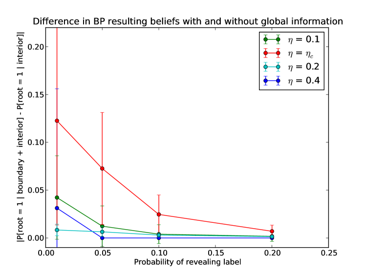
Figure 2: The average distance $|p_{R,L}-p_{R}|$ is shown for $\eta=0.1,\eta_{c},0.3,0.4$ and $p=0.01,0.05,0.1,0.2$.

References

- [1] Armen E. Allahverdyan, Greg Ver Steeg, and Aram Galstyan. Community detection with and without prior information. Europhysics Letters, 90:18002, 2010.
- [2] Krishna B. Athreya and Peter E. Ney. Branching Processes. Springer Berlin, 1972.
- [3] Sugato Basu, Arindam Banerjee, and Raymond J Mooney. Semi-supervised clustering by seeding. In ICML, volume 2, pages 27–34, 2002.
- [4] Sugato Basu, Mikhail Bilenko, and Raymond J. Mooney. A probabilistic framework for semi-supervised clustering. In Proceedings of the tenth ACM SIGKDD international conference on Knowledge discovery and data mining, pages 59–68. ACM, 2004.
- [5] P. J. Bickel and A. Chen. A nonparametric view of network models and Newman-Girvan and other modularities. Proceedings of the National Academy of Science, 106(50):21068–21073, 2009.
- [6] Olivier Chapelle, Jason Weston, and Bernhard Schoelkopf. Cluster kernels for semi-supervised learning. In NIPS, pages 585–592, 2002.
- [7] A. Coja-Oghlan. Graph partitioning via adaptive spectral techniques. Combinatorics, Probability and Computing, 19(02):227–284, 2010.
- [8] A. Condon and Richard M. Karp. Algorithms for graph partitioning on the planted partition model. Random Structures and Algorithms, 18(2):116–140, 2001.
- [9] Aurelien Decelle, Florent Krzakala, Cristopher Moore, and Lenka Zdeborová. Asymptotic analysis of the stochastic block model for modular networks and its algorithmic applications. Phys. Rev. E, 84:066106, Dec 2011.
- [10] Aurelien Decelle, Florent Krzakala, Cristopher Moore, and Lenka Zdeborová. Inference and phase transitions in the detection of modules in sparse networks. Phys. Rev. Lett., 107:065701, 2011.
- [11] Martin E. Dyer and Alan M. Frieze. The solution of some random NP-hard problems in polynomial expected time. Journal of Algorithms, 10(4):451–489, 1989.
- [12] William Evans, Claire Kenyon, Yuval Peres, and Leonard J. Schulman. Broadcasting on trees and the Ising model. The Annals of Applied Probability, 10(2):410–433, 2000.
- [13] David Gamarnik and Madhu Sudan. Limits of local algorithms over sparse random graphs. In Proceedings of the 5th conference on Innovations in theoretical computer science, pages 369–376. ACM, 2014.
- [14] Hamed Hatami, László Lovász, and Balázs Szegedy. Limits of local-global convergent graph sequences. arXiv preprint arXiv:1205.4356, 2012.
- [15] P. W. Holland, K. B. Laskey, and S. Leinhardt. Stochastic blockmodels: First steps. Social Networks, 5(2):109–137, 1983.
- [16] Mark Jerrum and G. B. Sorkin. The Metropolis algorithm for graph bisection. Discrete Applied Mathematics, 82(1–3):155–175, 1998.
- [17] David A. Levin, Yuval Peres, and Elizabeth L. Wilmer. Markov chains and mixing times. American Mathematical Society, 2006.
- [18] Russell Lyons and Fedor Nazarov. Perfect matchings as iid factors on non-amenable groups. European Journal of Combinatorics, 32(7):1115–1125, 2011.
- [19] Laurent Massoulié. Community detection thresholds and the weak Ramanujan property. In Proceedings of the Symposium on the Theory of Computation (STOC), 2014.
- [20] Frank McSherry. Spectral partitioning of random graphs. In Proceedings of IEEE Conference on the Foundations of Computer Science (FOCS), pages 529–537, 2001.
- [21] Elchanan Mossel. Reconstruction on trees: Beating the second eigenvalue. The Annals of Applied Probability, 11(1):285–300, 2001.
- [22] Elchanan Mossel. Survey: Information flow on trees. Available at arxiv.org/abs/math/0406446, 2004.
- [23] Elchanan Mossel, Joe Neeman, and Allan Sly. Stochastic block models and reconstruction. Preprint avaiable at arxiv.org/abs/1202.1499, 2012.
- [24] Elchanan Mossel, Joe Neeman, and Allan Sly. Belief propogation, robust reconstruction, and optimal recovery of block models. Preprint available at arxiv.org/abs/1309.1380, 2013.
- [25] Elchanan Mossel, Joe Neeman, and Allan Sly. A proof of the block model threshold conjecture. Preprint available at http://arxiv.org/abs/1311.4115, 2013.
- [26] Elchanan Mossel and Yuval Peres. Information flow on trees. Ann. Appl. Probab., 13(3):817–1230, 2003.
- [27] A. Sly. Reconstruction of symmetric potts models. In Proceedings of the 41st ACM Symposium on Theory of Computing, pages 581–590, 2009.
- [28] T. A. B. Snijders and K. Nowicki. Estimation and prediction for stochastic blockmodels for graphs with latent block structure. Journal of Classification, 14(1):75–100, 1997.
- [29] Greg Ver Steeg, Cristopher Moore, Aram Galstyan, and Armen E. Allahverdyan. Phase transitions in community detection: A solvable toy model. Available at http://www.santafe.edu/media/workingpapers/13-12-039.pdf, 2013.
- [30] Pan Zhang, Florent Krzakala, Jörg Reichardt, and Lenka Zdeborová. Comparitive study for inference of hidden classes in stochastic block models. Journal of Statistical Mechanics : Theory and Experiment, 2012.
- [31] Pan Zhang, Cristopher Moore, and Lenka Zdeborová. Phase transitions in semisupervised clustering of sparse networks. Available at http://arxiv.org/abs/1404.7789, 2014.