Demystifying the Scaling Laws of Dense Wireless Networks: No Linear Scaling in Practice

Abstract

We optimize the hierarchical cooperation protocol of Ozgur, Leveque and Tse, which is supposed to yield almost linear scaling of the capacity of a dense wireless network with the number of users $n$. Exploiting recent results on the optimality of “treating interference as noise” in Gaussian interference channels, we are able to optimize the achievable average per-link rate and not just its scaling law. Our optimized hierarchical cooperation protocol significantly outperforms the originally proposed scheme. On the negative side, we show that even for very large $n$, the rate scaling is far from linear, and the optimal number of stages $t$ is less than 4, instead of $t\rightarrow\infty$ as required for almost linear scaling. Combining our results and the fact that, beyond a certain user density, the network capacity is fundamentally limited by Maxwell laws, as shown by Francheschetti, Migliore and Minero, we argue that there is indeed no intermediate regime of linear scaling for dense networks in practice.

I Introduction

Although it is extremely hard to characterize the exact capacity of wireless networks, much progress has been made recently in the understanding of their theoretical limits. In [1], a hierarchical protocol named hierarchical cooperation was proposed by combining local communication and long-range cooperative MIMO communication. Applying $t$ stages of the basic cooperative scheme to a dense network with $n$ users in a hierarchical architecture, a capacity scaling of $\Theta(n^{\frac{t}{t+1}})$ was shown to be achievable. Therefore, for any $\epsilon>0$, any scaling of $\Theta(n^{1-\epsilon})$ is achievable for sufficiently large $t$. Such “linear scaling” of the network capacity with the number of users $n$ is the holy grail of large wireless networks since it yields constant average rate per source-destination pair in the case where sources and destinations are randomly selected such that their distance is $O(1)$. This, in turn, implies that the network is “scalable” since the rate per end-to-end communication session does not vanish as the number of users grow. In contrast, well-known protocols such as “decode and forward” (aka, multi-hop routing) yield the well known scaling of $\Theta(\sqrt{n})$ [2].

While scaling law analysis yields nice and clean results, it is hard to tell how a network really performs in terms of rates, since they fail to characterize the constants of the leading term in $n$ versus the next significant terms. Therefore, there might be significant regimes where the linear scaling does not manifest. The purpose of this paper is twofold. First, we derive an achievable sum-rate (not just a scaling law) for the hierarchical cooperation protocol. Second, we optimize the scheme on the basis of the achievable sum-rate, by appropriately choosing the transmit power, reuse factor, and quantization distortion level.

System model: We consider a network deployed over a unit-area squared region and formed by $n$ nodes placed on a regular grid with minimum distance $1/\sqrt{n}$. The grid topology captures the essence of the problem while avoiding some technicalities due to node random placement. The network consists of $n$ source-destination pairs, such that each node is both a source and a destination, and pairs are selected at random over the set of $n$-permutation $\pi$ that do not fix any element (i.e., for which $\pi(i)\neq i$ for all $i=1,\ldots,n$). We focus on max-min fairness, such that all source-destination pairs wish to communicate at the same rate. The channel coefficient between a transmitter node $k$ and a receive node $\ell$ at distance $r_{\ell k}$ is given by $h_{\ell k}=r_{\ell k}^{-\alpha/2}\exp{(j\theta_{\ell k})}$, where $\alpha$ denotes the path-loss exponent and $\theta_{\ell k}\sim\mbox{Unif}(0,2\pi]$ denotes a random i.i.d. phase. This independent “phase fading” model is the same assumed in [1].

Discussion and overview of the results: This work gives an answer to the question of “Is linear scaling achievable in practice?” Consider a wireless network operating on a university campus of area ${\cal A}=1\mbox{km}^{2}$. When operating around 30 GHz (i.e., $\lambda=0.01$m), the number of spatial degrees of freedom is given by $\sqrt{{\cal A}}/\lambda=10^{5}$ [3]. Then, we can expect almost linear scaling up to $10^{5}$ students using hierarchical cooperation protocol in [1]. However, we show that for $n\leq 10^{5}$, the optimal number of stages $t$ is less than $4$, i.e., the rate scaling is far from linear, which is in accordance with a previous result in [4], based on the scaling law analysis, where the optimal number of stages is found to be $O(\sqrt{\log{n}})$. This apparent contradiction can be understood as follows. The linear scaling in [1] is obtained by letting first $n\rightarrow\infty$ to get the scaling law of the single stage, and then $t\rightarrow\infty$ to achieve the linear scaling. In contrast, this work starts from a network density $n$ and for each $n$, we find the optimal number of hierarchical stages $t$ in terms of sum-rate, essentially capturing the impact of a finite network size. We refer the reader to the full manuscript [5] for the detailed proofs of our results. Further, it is shown in [5] that our optimized hierarchical cooperation scheme outperforms the classical multi-hop routing for a moderately large network size (i.e., $n\approx 10^{4}$), having a larger and larger gain as network size increases.

II Cooperative Transmission Scheme

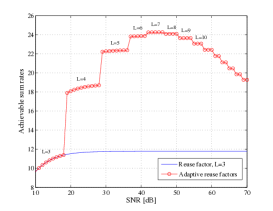
Figure 1: Achievable sum-rates of the cooperative transmission scheme when $\alpha=3$ and $n=10^{4}$.

In this section, we optimize the cooperative transmission scheme proposed in [1] with respect to the achievable sum-rate. We let $R_{{\rm c}}(\alpha)$ denote the common message coding rate for all users, expressed in bits per codeword symbol. The protocol delivers $n$ messages using a certain number of time-slots, each of which corresponds to the duration of a codeword. Hence, the network sum throughput is given by $R_{\rm sum}(n,\alpha)=R_{{\rm c}}(\alpha)\mbox{T}(n,\alpha)$ where $\mbox{T}(n,\alpha)=n/\mbox{(required number of time slots)}$ is the source-destination links per time slot ratio of the protocol (referred to as packet throughput in the following). The network is divided into $n/M$ clusters, of $M$ nodes each. The cooperative transmission scheme consists of three phases: 1) A “local” communication phase is used to form cooperative clusters of transmitters. In this phase, each source distributes $M$ distinct sub-packets of its message to the $M$ neighboring nodes in the same cluster. One transmission is active per each cluster, in a round robin fashion, and clusters are active simultaneously in order to achieve some spatial spectrum reuse. The inter-cluster interference is controlled by the reuse factor $L$; 2) A “global” cooperative MIMO transmission phase is used to deliver messages across different clusters. In this phase, one cluster at a time is active, and when a cluster is active it operates as a single $M$-antenna MIMO transmitter, sending $M$ independently encoded data streams to a destination cluster. Each node in the cooperative receiving cluster stores its own received signal; 3) A “local” communication phase during which all receivers in each cluster share their own received and quantized signals in order to allow each destination in the cluster to decode its intended message on the basis of the (quantized) $M$-dimensional observation. Quantization and binning (or random hashing of the quantization bits onto channel codewords) is used in this phase, which is a special case of the general Quantize reMap and Forward (QMF) scheme for wireless relay networks [6]. Each destination performs joint typical decoding to obtain its own desired message based on the quantized signals (or bin indices).

The parameters we need to optimize in the cooperative transmission scheme are the cluster size $M$, the node transmit power ${\sf SNR}$, reuse factor $L$, and quantization distortion level. Regarding the transmit power, it is assumed that ${\sf SNR}$ can be chosen arbitrarily with a uniform bound ${\sf SNR}\leq{\sf SNR}_{\max}$ where the latter is a fixed arbitrarily large constant that does not scale with $n$. As the result of such optimization in Sections II-A, II-B, and II-C, we have:

Theorem 1

For any network size $n$ and path-loss exponent $\alpha$, the cooperative transmission scheme achieves the sum-rate of

$$R_{\rm sum}(n,\alpha)=\log\left(1+\frac{{\sf SNR}}{1+P_{I}}\right)\frac{\sqrt{n}}{2\sqrt{2}L({\sf SNR})}$$

where ${\sf SNR}=2^{2(3+\alpha/\ln{2})}$, $L({\sf SNR})=\left\lceil\sqrt{{\sf SNR}}^{1/\alpha}+1\right\rceil$, and $P_{I}=\sum_{i=1}^{\sqrt{n}}8i{\sf SNR}(L({\sf SNR})-1)^{-\alpha}$. ∎

Theorem 1 implies that all sources can reliably transmit their messages at rate $R_{{\rm c}}(\alpha)\approx\log{\sqrt{{\sf SNR}}}$ over the $2\sqrt{2}L({\sf SNR})\sqrt{n}$ time slots. Notice that despite the fact we let ${\sf SNR}_{\max}$ to be an arbitrarily large constant, the optimal SNR depends only on the pathloss $\alpha$ and it is generally not too large. This is because there is a tension between the transmit power of each local link and the reuse factor necessary to keep inter-cluster interference under control. The optimal transmit power is determined in Section II-C (Theorem 1), as a result of this tradeoff. For comparison, notice that in the original scheme of [1] the reuse factor is fixed to 3. Fig. 1 shows that our optimized scheme provides a substantial gain over the conventional scheme [1].

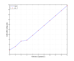
Figure 2: Achievable coding rates of hierarchical cooperation protocol as a function of path-loss exponent $\alpha$.

II-A Local Communication

In phases 1 and 3 of the scheme there is no intra-cluster interference since a single transmitter-receiver pair is active in each cluster. However, each receiver suffers from inter-custer interference from the transmitters in the other clusters. Hence, we are in the presence of a $n/M$ user (symmetric) interference channel. It has been recently recognized that there exists a regime of the interference channel gains for which treating interference as noise (TIN) is information-theoretically optimal (to within a constant gap) [7, Theorem 4]. Furthermore, TIN is most attractive in practice since it requires standard “Gaussian” codes and minimum distance decoders. Hence, we shall operate the interference channel induced by the local communication phases in the regime for which TIN is (near) optimal. This can be obtained by choosing a reuse factor $L$ such that the TIN optimality condition on the channel coefficients of the simultaneously active links is satisfied. We first determine the transmit power $P$ according to the cluster area ${\cal A}$ and the path-loss exponent $\alpha$ as $P={\sf SNR}{\cal A}^{\alpha/2}$. This choice makes that ${\sf SNR}_{i}={\sf SNR}$ for all $i$ where ${\sf SNR}_{i}$ denotes the received power of desired signal at node $i$. Also, let ${\sf INR}$ denote the strongest interference power, i.e., ${\sf INR}=\max_{j\neq i}{\sf INR}_{ij}=\max_{k\neq i}{\sf INR}_{ki}$, where ${\sf INR}_{ij}$ denote the interference-to-noise ratio of source $j$ at destination $i$ and the last equality is due to the symmetric structure of network. Considering the TDMA structure, we obtain that ${\sf INR}=(L-1)^{-\alpha}{\sf SNR}$. In our symmetric model, the optimality condition of TIN [7] is satisfied if ${\sf INR}\leq\sqrt{{\sf SNR}}$. We can find $L$ to meet the above condition as $L({\sf SNR})=\left\lceil\sqrt{{\sf SNR}}^{1/\alpha}+1\right\rceil$. Then, the local communication rate of $R^{(1)}({\sf SNR})=\log\left(1+{\sf SNR}/(1+P_{I})\right)$ is achievable by TIN, where the inter-cluster total interference is upper bounded by $P_{I}$ defined in Theorem 1. Reliable local communication is ensured by letting:

$$R_{{\rm c}}(\alpha)\leq R^{(1)}({\sf SNR}).$$ (1)

II-B Long-Range MIMO Communication

Concatenating phases 2 and 3 is analogous to a distributed MIMO channel with finite backhaul capacity of rate $R_{0}$ [8, 9], where the $M$ transmit (resp., $M$ receiver) antennas correspond to the $M$ nodes in the source cluster (resp., destination cluster). For the MIMO transmission (i.e., phase 2), the transmit power is given by $P_{{\rm MIMO}}=({\sf SNR}^{\prime}/M){\cal A}^{\alpha/2}$ where ${\sf SNR}^{\prime}$ can be arbitrary chosen with ${\sf SNR}^{\prime}\leq{\sf SNR}_{\max}$ as before. Including the impact of distance-dependent power control into a channel, the channel matrix of distributed MIMO channel is ${\bf H}\in\mbox{\bb C}^{M\times M}$, with $(k,\ell)$-element given by $\exp(j\theta_{k\ell})$ with $\theta_{k\ell}\sim\mbox{Unif}(0,2\pi]$. Let $N_{0}$ denote the variance of additive noise plus inter-cluster interference. As in [1], the local communication of phase 3 can be expanded over $Q$ time slots for some integer $Q$, in order to obtain more flexibility in the quantization rate of the underlying QMF scheme. This yields the backhaul capacity of the “equivalent” model as $R_{0}=QR^{(1)}({\sf SNR})$. An optimal $Q$ will be chosen later on.

The computation of the rate achievable by QMF for the distributed MIMO channel with finite backhaul capacity is generally difficult since it involves a complicated combinatorial optimization [8]. So far, a closed-form expression was only available for the symmetric Wyner model [8]. In this paper, we derive a closed-form expression of the achievable rate for our model, exploiting the fact that, for large $n$, the problem symmetries although the matrix ${\bf H}$ is “full” and not tri-diagonal as in the Wyner model. Our result is based on asymptotic Random Matrix Theory and the submodular structure of rate expression:

Theorem 2

For a distributed MIMO channel with backhaul capacity of $R_{0}$ and random i.i.d. channel coefficients with zero mean and unit variance, QMF achieves the symmetric rate of

$$R_{{\rm QMF}}(R_{0},N_{0},{\sf SNR})$$

$$= \min\left\{R_{0}-\log\left(1+N_{0}/\sigma_{q}^{2}\right),{\cal C}\left({\sf SNR}/(N_{0}+\sigma_{q}^{2})\right)\right\}$$

for some quantization level $\sigma_{q}^{2}\geq 0$, where ${\cal C}(x)=2\log\left((1+\sqrt{1+4x})/2\right)-(\sqrt{1+4x}-1)^{2}\log{e}/4x$. ∎

Since the first rate-constraint is an increasing function of $\sigma_{q}^{2}$ and the second rate-constraint is a decreasing function of $\sigma_{q}^{2}$, the optimal value of $\sigma_{q}^{2}$ is attained by solving $R_{0}-\log\left(1+N_{0}/\sigma_{q}^{2}\right)={\cal C}\left({\sf SNR}/(N_{0}+\sigma_{q}^{2})\right)$. Define $h(\sigma_{q}^{2})\stackrel{{\scriptstyle\Delta}}{{=}}R_{0}-\log\left(1+N_{0}/\sigma_{q}^{2}\right)-{\cal C}\left({\sf SNR}/(N_{0}+\sigma_{q}^{2})\right)$. Then, we can find $\sigma_{q,{\rm min}}^{2}=N_{0}/(2^{R_{0}}-1)$ and $\sigma_{q,{\rm max}}^{2}=(N_{0}+{\sf SNR})/(2^{R_{0}}-1)$ such that $h(\sigma_{q,{\rm min}}^{2})\leq 0$ and $h(\sigma_{q,{\rm max}}^{2})\geq 0$. This is because $\sigma^{2}_{q,{\rm min}}$ makes the first rate-constraint in (2) zero and $\sigma^{2}_{q,{\rm max}}$ is the quantization level of Quantize and Forward (QF), which makes the second rate-constraint in (2) active. Using bisection method, we can quickly find an optimal quantization level $\sigma^{2}_{q,{\rm opt}}$ that will be used in this paper to plot the achievable rates of QMF.

Putting together the MIMO rate constraint of Theorem 2 with the rate achievable in phase 1 (1), we find $R_{{\rm c}}(\alpha)=\min\{R^{(1)}({\sf SNR}),R_{{\rm QMF}}(QR^{(1)}({\sf SNR}),1,{\sf SNR}^{\prime}))\}$. Since there is no inter-cluster interference (i.e., $N_{0}=1$) in the MIMO communication phase 2, we can find some finite value ${\sf SNR}^{\prime}$ with $Q=1$ such that $R^{(1)}({\sf SNR})\leq R_{{\rm QMF}}(R^{(1)}({\sf SNR}),1,{\sf SNR}^{\prime})$. Then, we have that $R_{{\rm c}}(\alpha)=R^{(1)}({\sf SNR})$, where an optimal ${\sf SNR}$ will be determined in the next section. In fact, we do not have to compute an exact achievable rate of QMF in this section but QMF rates will be used in Section III for the hierarchical cooperation protocol, when we shall consider multiple stages of the 3-phase cooperative scheme.

II-C Achievable sum-rate

In order to derive an achievable sum-rate, we will compute the packet throughput $\mbox{T}(n,\alpha)$. As anticipated before, in the cooperative scheme each source transmits $M$ distinct sub-packets of the message to the intended destination. To transmit overall $nM$ sub-packets (in the whole network), phase 1 requires the $(L({\sf SNR})M)^{2}$ time slots, phase 2 requires $n$ time slots, and phase 3 requires the $Q(L({\sf SNR})M)^{2}$ time slots. Based on this, we have $\mbox{T}(n,\alpha)=Mn/((Q+1)(L({\sf SNR})M)^{2}+n)$. Since the coding rate $R^{(1)}({\sf SNR})$ is independent of $M$, we can find the optimal cluster size $M$ by treating $M$ as a continuous variable and solving $d\mbox{T}(n,\alpha)/dM=0$. This yields $M=\sqrt{n}/(L({\sf SNR})\sqrt{1+Q})$. Then, the packet throughput is obtained as $\mbox{T}(n,\alpha)=\sqrt{n}/(2L({\sf SNR})\sqrt{1+Q})$ and accordingly, the achievable sum-rate is given by $R_{{\rm sum}}(n,\alpha)=R^{(1)}({\sf SNR})\sqrt{n}/(2L({\sf SNR})\sqrt{1+Q})$. Next, we will optimize the transmit power ${\sf SNR}$ to maximize the above sum-rate. To make the problem tractable, we use the approximations $L({\sf SNR})=\sqrt{{\sf SNR}}^{1/\alpha}$ and $R^{(1)}({\sf SNR})=\log(\sqrt{{\sf SNR}}/8)$. Then, the sum-rate is approximated by $\tilde{R}_{{\rm sum}}(n,\alpha)=\sqrt{n}\log(\sqrt{{\sf SNR}}/8)/(2\sqrt{2}\sqrt{{\sf SNR}}^{1/\alpha})$ where $Q=1$ is chosen because of the explanation given before. Differentiating and solving $d\tilde{R}_{{\rm sum}}(n,\alpha)/d{\sf SNR}=0$, we find that the optimal transmit power is given by ${\sf SNR}=2^{2(3+\alpha/\ln 2)}$.

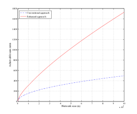
Figure 3: $\alpha=3$. Achievable sum-rates as a function of $n$.

III Optimizing the hierarchical cooperation protocol

Hierarchical cooperation was proposed in [1] by employing the cooperative transmission scheme of Section II as the local communication of a higher stage. In this scheme, we use the symmetric coding rate $R_{{\rm c}}(\alpha)$ regardless of the number of hierarchical stages $t$. Based on Section II, we choose $P_{i}={\sf SNR}{\cal A}_{i}^{\alpha/2}$, $L=\left\lceil\sqrt{{\sf SNR}}^{1/\alpha}+1\right\rceil$, and ${\sf SNR}=2^{2(3+\alpha/\ln{2})}$, for stages $i=1,\ldots,t$, where ${\cal A}_{i}$ denotes the cluster area of stage $i$. Notice that these choices guarantee that, regardless of hierarchical stage $i$, the received power of inter-cluster interference is at most equal to $P_{I}$ in Theorem 1. For the MIMO communication phase, we choose transmit power $P_{\mbox{{\tiny MIMO}},i}=({\sf SNR}/M){\cal A}_{i}^{\alpha/2}$, which also makes the interference power to be not larger than $P_{I}$. The following is the main result of this section:

Theorem 3

For any network size $n$ and path-loss exponent $\alpha$, the hierarchical cooperation protocol with $t\geq 2$ stages achieves the sum-rate of

$$R_{\rm sum}^{(t)}(n,\alpha)=R_{{\rm c}}(\alpha)n^{\frac{t}{t+1}}/\left((1+t)L^{\frac{2t}{t+1}}\sqrt{3}^{t}\right)$$

where $L=\left\lceil 2^{(3+\alpha/\ln{2})/\alpha}+1\right\rceil$ and $R_{{\tiny c}}(\alpha)$ is determined in Section III-A. Some coding rates $R_{{\rm c}}(\alpha)$ are provided for the interesting $\alpha$’s in Fig. 2.

Proof:

See Sections III-A and III-B. ∎

When $t=1$, the sum-rate in the above does not reduce to the previous result in Theorem 1 since in this case we can choose a higher coding rate than $R_{{\tiny c}}(\alpha)$ in Fig. 2, because there is no inter-cluster interference in the MIMO communication phase. From Theorem 3, we observe that a linear scaling can be achieved as $t\rightarrow\infty$ when the network size $n$ grows faster than the constant term $(1+t)L^{\frac{2t}{t+1}}\sqrt{3}^{t}$. However, for a finite network size, the constant term cannot be neglected since it also grows with $t$. Namely, adding more stages does not necessarily improve the achievable sum-rate. Thus, for given $n$, we can find an optimal number of hierarchical stages to maximize the sum-rate. In order to make the problem manageable, we relax the integer constraint on $t$ and find the optimal $t$ as solution of $dR_{{\rm sum}}^{(t)}(n,\alpha)/dt=0$. This gives the equation in $t$ as $(t+1)^{2}\ln{\sqrt{3}}+(t+1)-\ln(n/L)=0$, which yields $t_{{\rm opt}}=-1+(-1+\sqrt{1+2\ln(n/L)\ln{3}})/\ln{3}$. This shows the following negative result: even for $n$ as large as $10^{7}$, the optimal number of hierarchical stages is not larger than 4. Hence, for networks of reasonable size, the linear scaling law is a “myth”, even without considering the physical propagation limitations analyzed in [3]. Fig. 3 plots the achievable sum-rate of the hierarchical cooperation protocol with the optimal number of stages. The conventional scheme is the one presented in [1] and the enhanced scheme is the one presented in this paper with sum-rate in Theorem 3. In our scheme, we have modified the TDMA phases in order to reduce the transmission overhead (see Section III-B for details). We observe that the enhanced scheme provides a considerable gain over the conventional scheme, having a larger gap as $n$ increases. Nevertheless, the network throughput is clearly sub-linear even for the range of unreasonably large $n$ shown in the figure.

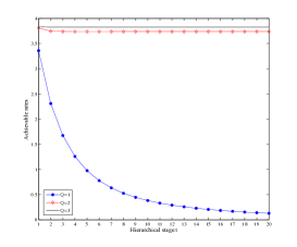
Figure 4: $\alpha=3$. Achievable coding rate as a function of hierarchical stage $t$.

III-A Achievable coding rate

From Section II, we have the rate-constraint of $R_{{\rm c}}(\alpha)\leq R^{(1)}\stackrel{{\scriptstyle\Delta}}{{=}}\log\left(1+{\sf SNR}/(1+P_{I})\right)$ for reliable local communication at the bottom stage (i.e., stage 1). Concatenating the phases 2 and 3 of stage 1, we can produce a distributed MIMO channel with backhaul capacity of $QR^{(1)}$ (see Section II-B). Then, the coding rate should satisfy the $R_{{\rm c}}(\alpha)\leq R_{{\rm QMF}}(QR^{(1)},N_{0}=P_{I}+1,{\sf SNR})\stackrel{{\scriptstyle\Delta}}{{=}}R^{(2)}$. Lemma 1 below yields that $R^{(2)}\leq R^{(1)}$ for any positive integer $Q\geq 1$. Since $R^{(2)}$ is the local communication rate of stage 2, we can produce a degraded distributed MIMO channel with backhaul capacity $QR^{(2)}\leq QR^{(1)}$, resulting in the rate-constraint $R_{{\rm c}}(\alpha)\leq R_{{\rm QMF}}(QR^{(2)},N_{0}=P_{I}+1,{\sf SNR})\stackrel{{\scriptstyle\Delta}}{{=}}R^{(3)}$. Clearly, we have that $R^{(3)}\leq R^{(2)}$. Repeating the above procedures, we obtain that $R^{(t+1)}\stackrel{{\scriptstyle\Delta}}{{=}}R_{{\rm QMF}}(QR^{(t)},P_{I}+1,{\sf SNR})\leq R^{(t)}$, such that $\{R^{(t)}\}$ is monotonically non-increasing. Hence, there exists a limit $\lim_{t\rightarrow\infty}R^{(t)}=R^{\star}(\alpha,Q)$, where such limit depends on $\alpha$ and $Q$. All rate-constraints are satisfied by choosing $R_{{\rm c}}(\alpha)=R^{\star}(\alpha,Q)$. One might have a concern that this choice is not a good one for small $t$. However, Fig. 4 shows that $R^{(t)}$ quickly converges to its positive limit for $Q\geq 2$. Also, we observe that $Q=2$ is the best choice since it almost achieves the upper bound $R^{(1)}$, by minimizing the required number of time slots. Therefore, we choose the $Q=2$ and $R_{{\rm c}}(\alpha)=R^{\star}(\alpha,2)$ in the following, for any $t$. The corresponding coding rates are plotted in Fig. 2 as a function of $\alpha$.

Lemma 1

For any $Q\geq 1$, the achievable rate of MIMO transmission is upper-bounded by the local communication rate of bottom stage (i.e., stage 1) as $R_{{\rm QMF}}(QR^{(1)},1+P_{I},{\sf SNR})\leq R^{(1)}$. ∎

III-B Achievable sum-rate

Focusing on the packet throughput, we first review the work in [1] and then improve it by efficiently using the TDMA scheme during the local communication phases.

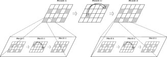
Figure 5: The silent features of the conventional scheme [1] for $t=2$.

Approach in [1]: The operation of stage 1 is equivalent to the cooperative transmissions and thus, from Section II-C, the packet throughput is computed as $\mbox{T}^{(1)}(n,\alpha)=\sqrt{n}/(2L\sqrt{1+Q})$. Also, stage 2 employs stage 1 as its local communication (see Fig. 5). Then, the required number of time slots is $(LM_{1})^{2}/\mbox{T}^{(1)}(M_{1},\alpha)$ for phase 1, $n$ for phase 2, and $Q(LM_{1})^{2}/\mbox{T}^{(1)}(M_{1},\alpha)$ for phase 3. With the optimal cluster size $M_{1}=n^{2/3}/(L^{2}(1+Q))$, the resulting packet throughput is given by $\mbox{T}^{(2)}(n,\alpha)=n^{2/3}/(3(L\sqrt{1+Q})^{2})$. Generalizing to $t$ stages, we obtain the achievable sum-rate of the scheme in [1] as $R_{{\rm sum}}^{(t)}(n,\alpha)=R_{{\rm c}}(\alpha)n^{t/(t+1)}/((t+1)(L\sqrt{1+Q})^{t})$.

Enhanced approach: We will improve the penalty term associated with TDMA from $L^{t}$ to $L^{\frac{2t}{t+1}}$. This provides a non-trivial gain especially when $t$ is large, since the former exponentially increases with $t$ while the latter is upper bounded by $L^{2}$. We explain our approach based on a 2-stage hierarchical cooperation protocol (see Fig. 6) and then extend the result to general $t$. First, we want to emphasize that TDMA scheme is used so that the received power of interference is less than a certain level for all transmissions. It can be noticed that this requirement is satisfied for the transmissions of phase 11 (or phase 13) (i.e., stage 1, phases 1 and 3) without using the TDMA scheme of phase 21 (stage 2, phase 1) since local communications have already included the TDMA operation. However, the TDMA scheme of phase 21 is required for the long-range MIMO communication of phase 12. Based on this observation, we present an alternative approach to efficiently use the TDMA scheme (see Fig. 6): All clusters in phase 21 (or phase 23) are always active (spatial reuse 1); In phase 12, each cluster has a turn to perform the MIMO transmissions every $L^{2}$ time slots, which is equivalent to apply the TDMA scheme of phase 21 (or phase 23). In short, this approach applies the TDMA scheme only once to every phase. Then, we can recompute the required number of time slots as follows. Since TDMA scheme is used for all phases in stage 1, it requires the $(LM_{1})^{2}+L^{2}n+Q(LM_{1})^{2}$ time slots. With the optimal cluster size $M_{1}=\sqrt{M_{2}}/\sqrt{1+Q}$, we can compute the packet throughput for local communication as $\mbox{TL}^{(1)}(M_{2})=\sqrt{M_{2}}/(2L^{2}\sqrt{1+Q})$, yielding the achievable sum-rate:

$$R_{{\rm sum}}^{(2)}(n,\alpha)=R_{{\rm c}}(\alpha)\frac{nM_{2}}{(1+Q)M_{2}^{2}/\mbox{TL}^{(1)}(M_{2})+n}$$

where TDMA is not used in this stage, as shown in Fig. 6. With the optimal cluster size $M_{2}=n^{2/3}/(L^{4/3}(1+Q))$, we have $R_{{\rm sum}}^{(2)}(n,\alpha)=R_{{\rm c}}(\alpha)n^{2/3}/\left(3L^{4/3}(1+Q)\right)$. Similarly, generalizing to a $t$-stage hierarchical protocol, we obtain:

$$R_{{\rm sum}}^{(t)}(n,\alpha) = R_{{\rm c}}(\alpha)\frac{nM_{t}}{(1+Q)M_{t}^{2}/\mbox{TL}^{(t-1)}(M_{t})+n}$$

$$\stackrel{{\scriptstyle(a)}}{{=}} R_{{\rm c}}(\alpha)\frac{nM_{t}}{n+tL^{2}(\sqrt{1+Q})^{t+1}M_{t}^{(t+1)/t}}$$

$$\stackrel{{\scriptstyle(b)}}{{=}} R_{{\rm c}}(\alpha)\frac{n^{\frac{t}{t+1}}}{(1+t)L^{\frac{2t}{t+1}}(\sqrt{1+Q})^{t}}$$

where (a) is from Lemma 2 below and (b) is from the optimal cluster size $M_{t}=\left(n/(L^{2}(\sqrt{1+Q})^{t+1})\right)^{t/(t+1)}$.

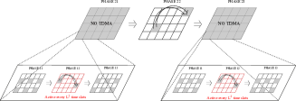
Figure 6: The silent features of the enhanced scheme for $t=2$.

Lemma 2

The packet throughput of local communication of stage-$t$ is given by $\mbox{TL}^{(t)}(n)=n^{\frac{t}{t+1}}/\left((t+1)L^{2}\sqrt{1+Q}^{t}\right)$. ∎

References

- [1] A. Ozgur, O. Leveque, and D. Tse, “Hierarchical Cooperation Achieves Optimal Capacity Scaling in Ad Hoc Networks,” IEEE Transactions on Information Theory, vol. 53, pp. 3549-3572, Oct. 2007.
- [2] P. Gupta and P. R. Kumar, “The capacity of wireless networks,” IEEE Transactions on Information Theory, vol. 42, pp. 388-404, Mar. 2000.
- [3] M. Franceschetti, M. D. Migliore, and P. Minero, “The capacity of wireless networks: Information-theoretic and physical limits,” IEEE Transactions on Information Theory, vol. 55, pp. 3413-3424, Aug. 2009.
- [4] J. Ghaderi, L.-L. Xie, and X. Shen, “Hierarchical Cooperation in Ad Hoc Networks: Optimal Clustering and Achievable Throughput,” IEEE Transactions on Information Theory, vol. 55, pp. 3425-3436, Aug. 2009.
- [5] S.-N. Hong and G. Caire, “On the Performance of Dense Wireless Networks: No Linear Scaling in Practice,” [Online] http://arxiv.org/abs/1402.1815.
- [6] S. Avestimehr, S. Diggavi, and D. Tse, “Wireless network information flow: A deterministic approach,” IEEE Transactions on Information Theory, vol. 57, pp. 1872-1905, Apr. 2011.
- [7] C. Geng, N. Naderializadeh, A. S. Avestimehr, and S. A. Jafar, “On the Optimality of Treating Interference as Noise,” [Online] http://arxiv.org/abs/1305.4610.
- [8] A. Sanderovich, O. Somekh, H. V. Poor, and S. Shamai (Shitz), “Uplink Macro Diversity of Limited Backhaul Cellular Network,” IEEE Transactions on Information Theory, vol. 55, pp. 3457-3478, Aug. 2009.
- [9] S.-N. Hong and G. Caire, “Compute-and-Forward Strategies for Cooperative Distributed Antenna Systems,” IEEE Transactions on Information Theory, vol. 59, pp. 5227-5243, Aug. 2013.