RR Lyrae in XSTPS: The halo density profile in the North Galactic Cap

Abstract

We present a catalog of RR Lyrae stars (RRLs) observed by the Xuyi Schmidt Telescope Photometric Survey (XSTPS). The area we consider is located in the North Galactic Cap, covering $\approx 376.75~{}\mathrm{deg}^{2}$ at $\alpha\approx 150~{}\mathrm{deg}$ and $\delta\approx 27~{}\mathrm{deg}$ down to a magnitude limit of $i\approx 19$. Using the variability information afforded by the multi-epoch nature of our XSTPS data, combined with colors from the Sloan Digital Sky Survey, we are able to identify candidate RRLs. We find 318 candidates, derive distances to them and estimate the detection efficiency. The majority of our candidates have more than 12 observations and for these we are able to calculate periods. These also allows us to estimate our contamination level, which we predict is between 30% to 40%. Finally we use the sample to probe the halo density profile in the $9-49~{}\mathrm{kpc}$ range and find that it can be well fitted by a double power law. We find good agreement between this model and the models derived for the South Galactic Cap using the Watkins et al. (2009) and Sesar et al. (2010) RRL data-sets, after accounting for possible contamination in our data-set from Sagittarius stream members. We consider non-spherical double power law models of the halo density profile and again find agreement with literature data-sets, although we have limited power to constrain the flattening due to our small survey area. Much tighter constraints will be placed by current and future wide-area surveys, most notably ESA’s astrometric Gaia mission. Our analysis demonstrates that surveys with a limited number of epochs can effectively be mined for RRLs. Our complete sample is provided as accompanying online material.

1. Introduction

Modern theories of galaxy formation and evolution predict that galaxies are formed by gradual accretion of baryonic matter falling into the gravitational potential of surrounding cold dark matter haloes (see Freeman & Bland-Hawthorn 2002 for a review). In this view large galaxies such as the Milky Way grow by accreting material from smaller nearby galaxies, which are tidally destroyed by the gravitational pull of the larger ones. Over cosmic time these small galaxies are therefore fragmented and reduced to clumps and streams of stars in the halo of the larger disrupting galaxy; these streams and clumps can in principle be detected by large scale surveys of the stellar halo of the large galaxy, allowing the theory to be tested. The test can be more easily carried out in the Milky Way halo. In the last decade or so considerable progress has been made thanks to the unprecedented capabilities of modern astronomical instrumentation that are now able to survey large portions of the Milky Way halo providing accurate photometric and spectroscopic data for millions of its stars.

Foremost among the large scale surveys of the halo has been the Sloan Digital Sky Survey (SDSS: York et al., 2000) whose data-set provides, among many other things, accurate photometric data in five bands for millions and spectra for hundreds of thousand of stars in the Milky Way. This data-set has been successfully used to study the Milky Way in great detail and on a large scale, both in the disk (e.g. Ivezić et al., 2008; Jurić et al., 2008; Bond et al., 2010) and in the halo. With regard to the halo, which is the focus of this paper, notable examples of use of SDSS data include Newberg et al. (2002), who identify new structures in the halo Way from analyzing five million stars, Yanny et al. (2003), who find evidence for a ring of stars in the plane of the Milky Way at $\approx~{}18~{}\mathrm{kpc}$, and Belokurov et al. (2006), who use SDSS photometry to study Milky Way halo substructure in the area around the north Galactic cap

While these studies probe the structure of the Milky Way via its whole stellar population and use samples comprised of millions of stars, with all the problems the analysis of such large data-sets entails, other approaches focus on identifying suitable tracer populations and use those tracer populations to probe the structure. When tracers are used the key problem is of course to identify the tracer itself and show that it indeed traces the underlying stellar population; the advantage is that one typically deals with samples comprised of hundreds or thousands of stars as opposed to millions.

Once again SDSS has been instrumental in enabling this kind of analyses: for example Xue et al. (2008) use Blue Horizontal Branch (BHB) stars from SDSS to derive the rotation curve of the Milky Way up to $\approx 60~{}\mathrm{kpc}$ from the center and Smith et al. (2009) build a sample of $\approx 1700$ halo stars in the solar neighborhood and use it to constrain the halo velocity dispersion and to look for substructure in the halo, as predicted by theories of galaxy formation.

Although SDSS has proved very useful for studying the stellar halo, one drawback is that for the most part it lacks multi-epoch data (the exception to this being the $\approx 300~{}\mathrm{deg}^{2}$ square degree Stripe 82 region; see below). This means that if one is interested in probing the structure of the Milky Way using a tracer population of variable objects, the usefulness of SDSS is severely reduced since with single epoch data alone it is in general not feasible to ascertain the variable nature of an object

This is an important concern if one wants to use RR Lyrae stars (RRLs) as a halo tracer population to study the Milky Way stellar halo. RRLs are Horizontal Branch stars like the BHB stars mentioned above; they are old and metal poor like the general halo stellar population and therefore constitute an excellent tracer. Their most notable characteristic is that they are variable objects with a period in the $0.2-1~{}\mathrm{d}$ range but in $V$ they have the same absolute brightness modulo the effect of metallicity and this fact can be used to derive a distance to them; unlike Cepheids, RRLs are lacking in well calibrated Period-Luminosity relations, although progress is being made on that front (Cáceres & Catelan, 2008; Madore et al., 2013; Klein et al., 2014). For a review of the use of RRLs stars as distance indicators see Bono 2003a.

They are also abundant and relatively easy to find if accurate multi-epoch data are available, as shown by the microlensing experiments in the 1990s. The three main microlensing experiments (MACHO: Alcock et al., 1993), (OGLE: Udalski et al., 1992), (EROS: Aubourg et al., 1993) proved to be invaluable for the study of variable objects in the Magellanic Clouds and the Milky Way bulge thanks to the hundreds of epochs available in their data-sets for each object; large catalogs of RRLs feature prominently among the data products of these surveys (Alcock et al., 1998; Soszyński et al., 2009; Soszyñski et al., 2010; Soszyński et al., 2011). The key to finding RRLs in large numbers in these data-set is the availability of hundreds of epochs, which enables to unambiguously establish the variable nature of an object and to find the RRL period with great precision; this however is not possible with single (or few) epoch data-sets such as SDSS.

In a pioneering paper Ivezić et al. (2005) show how RRLs can be reliably identified in the SDSS data-set by a combination of color cuts, even with few (or just one) epochs; in particular the cuts they propose are:

$$14<r < 20,$$

$$0.98<u-g < 1.3,$$

$$D_{ug}\equiv(u-g)+0.67(g-r) - 1.07,$$

$$D_{gr}\equiv 0.45(u-g)-(g-r) - 0.12,$$

$$D_{ug}^{\mathrm{Min}}<D_{ug} < 0.35,$$

$$D_{gr}^{\mathrm{Min}}<D_{gr} < 0.55,$$

$$-0.15<r-i < 0.22,$$

$$-0.21<i-z < 0.25$$ (1)

where $D_{ug}^{\mathrm{Min}}$ and $D_{gr}^{\mathrm{Min}}$ can be chosen to give a desired selection completeness and efficiency. Ivezić et al. (2005) however show that, for a complete RRL sample, their selection efficiency is only $6\%$ (this efficiency may be increased at the price of reduced completeness with different cuts), that is, in a color-selected sample that includes all RRLs, these will make up just $6\%$ of the selected objects. It is therefore necessary that studies of the Milky Way halo based on RRLs should include criteria other than the cuts in Equations 1 to cleanly select a contamination free sample; such criteria usually exploit the availability of multi-epoch and multi-band photometry (though much fewer epochs than the microlensing searches are needed).

While most SDSS fields have been in general observed once or few times, this is not the case for a particular region in the South Galactic Cap (SGC) known as Stripe 82 which has accurate five band and multi-epoch photometry. SDSS Stripe 82 has therefore been the object of much recent work aimed at efficiently detecting variable objects, including RRLs, using combinations of color cuts and variability information provided by sparsely sampled light-curves (typically objects in Stripe 82 have light-curves with at most a few tens of points, as opposed to the several hundreds or even thousands of points in microlensing searches). Sesar et al. (2007) investigate the problem of detecting variable objects with just as few multi band photometric measurements as four and propose a series of criteria they apply to variable objects in Stripe 82.

Using these criteria and the cuts in Equations 1 with $D_{ug}^{\mathrm{Min}}=-0.05~{}\mathrm{mag}$ and $D_{gr}^{\mathrm{Min}}=0.06~{}\mathrm{mag}$ Sesar et al. (2007) also select 683 RRL candidates from Stripe 82 and use it to investigate the structure of the Milky Way halo down to $\approx 100~{}\mathrm{kpc}$; however this sample still suffers from contamination due to the generally low number of available observations.

Watkins et al. (2009, hereafter W09) use the same set of color cuts, with the same $D_{ug}^{\mathrm{Min}}$ and $D_{gr}^{\mathrm{Min}}$ and slightly different criteria for detecting variability, and look for RRLs in Stripe 82 using the light motion catalog presented by Bramich et al. (2008). W09 find 407 RRLs (316 RRab and 91 RRc) and detect over-densities in the Milky Way halo, including a newly discovered one at $\approx 80~{}\mathrm{kpc}$, $l\approx 80~{}\mathrm{deg}$, $b\approx-55~{}\mathrm{deg}$ which they term the Pisces Overdensity.

Using additional data in Stripe 82 from the SDSS Supernova Survey (Frieman et al., 2008; Sako et al., 2008) Sesar et al. (2010, hereafter S10) update the analysis performed in (Sesar et al., 2007) and present a new catalog composed of 483 objects; S10 note that, while the main conclusions of Sesar et al. (2007) are still valid, only $\approx 70\%$ of Sesar et al. (2007) RRL candidates turn out to be true RRL in S10, with the majority of the other candidates turning out to be $\delta$ Scuti stars. By taking advantage of the high temporal cadence afforded by the SDSS Supernova Survey S10 are also able to construct detailed light-curve templates in the five SDSS bands; this improved sampling also allows S10 to relax their color cuts from $u-g>0.98~{}\mathrm{mag}$ to $u-g>0.7~{}\mathrm{mag}$ to better find low metallicity RRLs.

Several RRL samples not using SDSS data have also been published in recent years. The QUEST RRL survey (Vivas et al., 2004) found 498 RRLs in a $380~{}\mathrm{deg}^{2}$ area from $4^{\mathrm{h}}.1$ to $6^{\mathrm{h}}.1$ and from $8^{\mathrm{h}}$ to $17^{\mathrm{h}}$ at $\delta\approx-1~{}\mathrm{deg}$, in the $13.5~{}\mathrm{mag}<V<19.5~{}\mathrm{mag}$ range, which allows them to probe the structure of the halo from $\approx 4~{}\mathrm{kpc}$ to $\approx 60~{}\mathrm{kpc}$. Using this data-set Vivas & Zinn (2006) investigate over-densities in the halo: they find that away from major over-densities the halo can be well fitted by a smooth, non-spherical (oblate) profile and use this profile to estimate a “background” and to look for over-densities overlaid on top of it.

Kinemuchi et al. (2006) present a sample of 1197 candidate RRLs in the solar neighborhood from the Northern Sky Variability Survey (NSVS). Keller et al. (2008) present 2016 candidate RRLs from the Southern Edgeworth-Kuiper Belt Object (Moody et al., 2003) (SEKBO) survey up to $\approx~{}50~{}\mathrm{kpc}$ and map halo over-densities, revealing a series of structures coincident with the leading and trailing arms of debris from the Sagittarius dwarf galaxy. Akhter et al. (2012) use the Keller et al. (2008) sample to study the steepening of the RRL distribution power-law slope beyond a Galacto-centric radius of $\approx~{}45~{}\mathrm{kpc}$ and find evidence for a change from $2.78\pm 0.02$ in the inner halo to $-5.0\pm 0.2$ in the outer. Miceli et al. (2008) present a sample of 838 RRLab from the Lowell Observatory Near Earth Objects Survey Phase I (Bowell et al., 1995) (LONEOS-I) up to a galacto-centric distance of $30~{}\mathrm{kpc}$ and find evidence for dual-halo models of halo formation.

While this work was in preparation, two new catalogs of RRL have been assembled. Firstly the LINEAR survey (Sesar et al., 2011a) has been mined, resulting in a sample of around 5000 RRL (Sesar et al., 2013; Palaversa et al., 2013). This catalog was then used to investigate the properties and distributions of the various types of RRL, measuring the halo profile and searching for substructure in the nearby (5-30 kpc) stellar halo. Secondly, Drake et al. (2013a) has presented a sample of 12227 type-ab RRLs covering $\approx 20,000~{}\mathrm{deg}^{2}$ to heliocentric distances up to $60~{}\mathrm{kpc}$ assembled from public light-curves in the Catalina Survey Data Release 1, providing periods and distances, and revealing parts of the Sagittarius Stream at heliocentric distances $20$ to $60~{}\mathrm{kpc}$. Drake et al. (2013b) use 1207 RRLs found in photometry from the Catalina Survey’s Mount Lemmon Telescope to detect RRLs up to $100~{}\mathrm{kpc}$ and find evidence for a tidal stream beyond $100~{}\mathrm{kpc}$ overlapping the Sagittarius Stream system. In the near future many other surveys will be able to provide large catalogs of RRLs, for example the Palomar Transient Factory (PTF; Rau et al. 2009), Pan-STARRS (Kaiser et al., 2002) and Gaia (Bono, 2003b; Eyer et al., 2012).

In this paper we present a catalog of 318 candidate RRLs observed by the Xuyi Schmidt Telescope Photometric Survey of the Galactic Anti-Center (XSTPS-GAC, XSTPS for short from now on) and use this catalog to probe the halo density profile in the North Galactic Cap (NGC) up to $\approx 50~{}\mathrm{kpc}$. The survey area is covered by the Drake et al. (2013a) area so it is likely that (part of) the RRLs we present are also detected by them. The paper is organized as follows: Section 2 introduces the XSTPS survey, Section 3 describes our cuts for finding RRL candidates, Section 4 describes our efficiency estimation for finding the candidates, Section 5 describes our period finding procedure for those candidates with enough observations and also our sample contamination estimate, Section 6 describes our distance estimation. In Section 7 we use the XSTPS RRLs to investigate the halo density profile in the North Galactic Cap in the $10-49~{}\mathrm{kpc}$ range, and the W09 and S10 RRLs to do the same for the South Galactic Cap and compare the results; Subsection 7.1 deals with spherical halo models and Subsection 7.2 deals with non-spherical halo models. Finally Section 8 reports our conclusions.

We point out that in this paper we do not use any period-luminosity relationship to estimate distances to our RRLs, because the periods for many of our RRLs are poorly constrained due to having few observations in just one band. As pointed out above, progress is being made improving RRL period-luminosity relationships and some are now becoming available that can be applied to our catalog (for example Cáceres & Catelan, 2008). In Section 6 we quantify the uncertainty introduced by our distance estimation.

2. The Xuyi Schmidt Telescope Photometric Survey of the Galactic Anti-Center (XSTPS)

XSTPS is a three band photometric survey of the Milky Way anti-center carried out with the $1.2~{}\mathrm{m}$ Schmidt telescope at the Xuyi station of the Purple Mountain Observatory in China (Zhang et al., 2013) and completed in March 2011 (see Section 3 of Liu et al., 2013). The survey covers an area of $\approx 6,000~{}\mathrm{deg}^{2}$ in a region of the sky that, for the most part, is not covered by other large scale surveys. It is expected to detect $\approx 100$ million stars in $i$ and the first data release is due imminently (Yuan et al., in preparation); we used a preliminary version of the catalog for our study. The three bands employed in the survey are $g$, $r$, $i$, similar, but not identical, to the corresponding SDSS bands; the transformations between the XSTPS and the SDSS systems are given by Equations 2 and are valid both for reddened and unreddened magnitudes (Yuan, Liu, & Xiang, 2013):

$$g^{\mathrm{SDSS}} = g+0.144(g-i),$$

$$r^{\mathrm{SDSS}} = r+0.0680(r-i),$$

$$i^{\mathrm{SDSS}} = i+0.0224(g-i).$$ (2)

The exposure time is $90~{}\mathrm{sec}$ and the magnitude limit is $\approx 19\mathrm{mag}$ in $i$. The data used in this work are based on extended and multi-epoch observations toward the NGC during December-February 2010 and 2011; the extended survey area covers the range $119.7~{}\mathrm{deg}\lesssim\mathrm{RA}\lesssim 193.5~{}\mathrm{deg}$ in Right Ascension (RA) and $24.6~{}\mathrm{deg}\lesssim\delta\lesssim 29.7~{}\mathrm{deg}$ in Declination ($\delta$) for an area $\approx 376.75~{}\mathrm{deg}^{2}$. Most of the observations were carried out in the $i$ band.

Observations in the same band at different epochs were matched using a matching radius of $3~{}\mathrm{arcsec}$ (for a discussion of the XSTPS astrometric accuracy, see Zhang et al., 2014). The procedure yielded $\approx 4.2$ million matches in $i$, as well as $\approx 1.17$ million in $r$ and $\approx 0.5$ million in $g$, however many of these matches are not true objects but false sources that must be excluded. To filter out these false sources we required that, to be considered as a true object, a source must be detected in at least two epochs; this leaves us with $\approx 1.6$ million sources that we consider bona fide objects; while this cut may appear too severe (after all there are true sources observed in just one epoch), it has no consequences for the subsequent analysis, in which we will be interested in multi-epoch objects anyway. The histogram of the number of epochs for all the 4.2 million sources in the $i$ band (including the false ones) is shown in Figure 1; the high number of sources having one or two epochs is due to the aforementioned contamination from false sources.

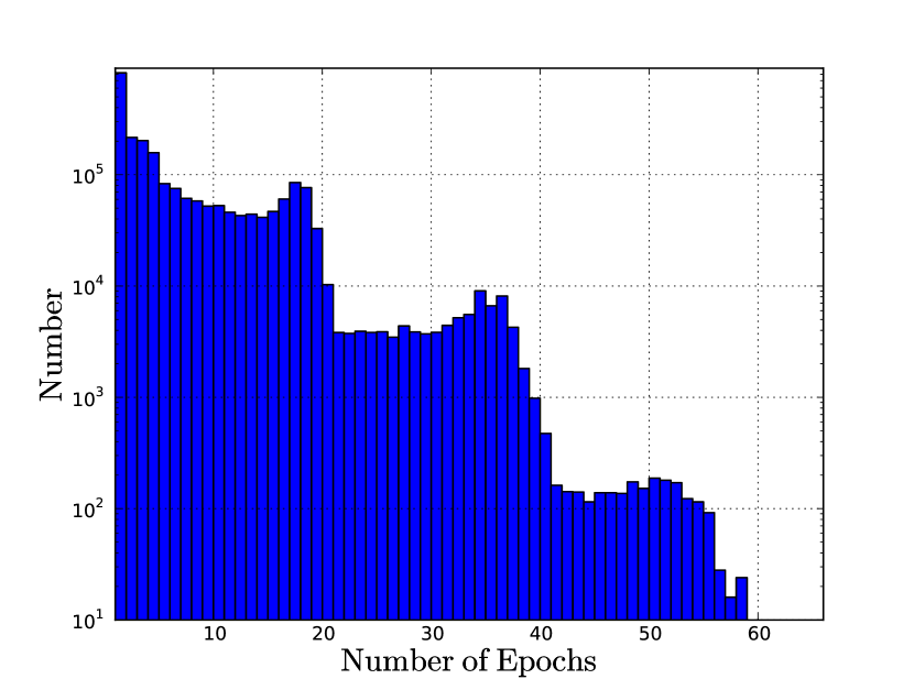
Figure 1.— Histogram of the number of epochs in the $i$ band.

Figure 2 shows the RMS $i$ magnitude $\sigma_{i}$ of 10,000 randomly selected objects with at least 10 epochs as a function of their mean $i$ magnitude. The figure shows that at $i\approx 19~{}\mathrm{mag}$, $\sigma_{i}\approx 0.1~{}\mathrm{mag}$; since typical RRL amplitudes can be as low as $0.3~{}\mathrm{mag}$ (Sesar et al., 2010), which corresponds to a RRL Amplitude-RMS magnitude ratio of just 3 at $19~{}\mathrm{mag}$, we take $19~{}\mathrm{mag}$ in $i$ as our completeness limit for the purpose of finding RRLs, consistent with the survey magnitude limit.

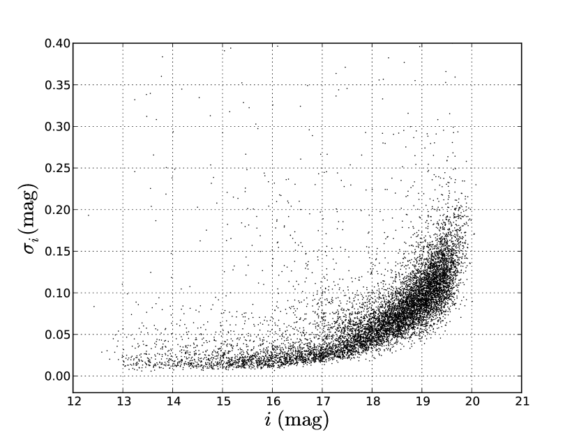
Figure 2.— RMS $i$ magnitude $\sigma_{i}$ of 10,000 randomly selected objects with at least 10 epochs as a function of their mean $i$ magnitude.

3. Finding RRLs in XSTPS

The method we used to select RRL candidates relies on a combination of SDSS colors as described by Equations 1 and variability information provided by the XSTPS data in this stripe. Therefore the first step is to select stars from SDSS in the region covered by the XSTPS stripe and cross correlate this sample with the XSTPS data. We selected objects in the SDSS Data Release 7 (DR7) from the “Star” table in the region $110~{}\mathrm{deg}<\mathrm{RA}<200~{}\mathrm{deg}$ and $24~{}\mathrm{deg}<\delta<30~{}\mathrm{deg}$ (J2000), with PSF $i_{\mathrm{SDSS}}$ magnitudes between $13.5$ and $22~{}\mathrm{mag}$. The query returned 2,445,651 objects that were correlated with the XSTPS $i^{\mathrm{SDSS}}$ band catalog in a $3~{}\mathrm{arcsec}$ radius; this gave $\approx 880,000$ matches for all the 4.2 millions of sources in the XSTPS data-set, including the false ones; we do not care about those at this stage since they will be filtered out later. We applied to these matches the cuts defined by Equations 1 with $D_{ug}^{\mathrm{Min}}=-0.05~{}\mathrm{mag}$ and $D_{gr}^{\mathrm{Min}}=0.06~{}\mathrm{mag}$ (Sesar et al., 2007) and found 12,992 stars with colors satisfying these these RRL cuts.

The next step in the process is to identify variable sources in the XSTPS data-set. Candidate variable sources were selected by first identifying objects with at least four epochs in the $i$ band (which yielded $\approx 1.1$ million objects and filtered out the false sources mentioned above, which usually have just one detection) and then fitting a constant to these objects and computing the $\chi^{2}$ fit statistic. Objects whose probability of having a $\chi^{2}$ equal to or higher than the one in the fit was $<0.001$ were considered potential variables; this cut yielded 19,556 objects. One particular concern with this procedure (especially so considering the low number of observations usually available) is that the $\chi^{2}$ may be high because of one single (or very few) discrepant point(s) due to bad observations. This was accomplished by refitting all the 19,556 candidate variables after removing each point in turn: if the low value of $\chi^{2}$ is due to a single point away from the others, a fit to a constant should give a good value of $\chi^{2}$ (defined as having a $0.2$ probability of $\chi^{2}$ being equal to or higher than the one in the fit) when this point is removed. In this case we may establish that the source is either a non RRL variable or is a constant with a bad point and we can exclude it from further consideration. Our cut removed $5,484$ sources from the list of candidate variables leaving $14,072$ objects that we consider bona fide variables. There is a chance that stars with a large number of epochs may have multiple bad observations, but this is dealt with later in Section 5.

We finally cross correlate the candidate RRLs found from the color cuts in Equations 1 with the sample of variables found via the criteria outlined in the above paragraph; this cross correlation finally yielded 318 objects that make up our candidate RRL sample. This sample includes a few objects with $i$ greater than our magnitude limit ($19~{}\mathrm{mag}$); these objects will not be used in subsequent analyses.

Our procedure for finding RRLs relies on detecting a poor fit to a constant baseline, so it is dependent on magnitude uncertainties since an object with a large uncertainty will be less likely to have a poor fit to a constant. It is therefore interesting to compare the uncertainty distribution as a function of magnitude of our RRL candidates with that of the general population of objects in the $i$ band from which the RRL sample is extracted. Figure 3 shows mean $i$ uncertainty versus $i$ magnitude for our RRL candidates and for 10,000 randomly chosen objects detected in the $i$ band.

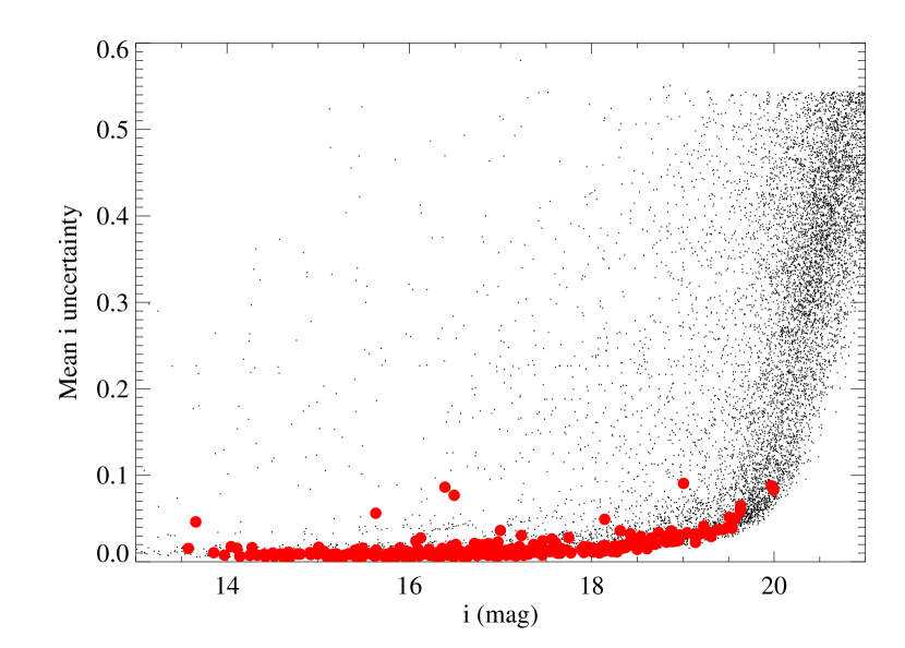
Figure 3.— Uncertainty on $i$ magnitude for our 318 RRL candidates (red points) and for 10,000 randomly selected objects in $i$ (small black points).

The figure shows that the two distributions are compatible down to our magnitude limit $i=19$ mag; beyond that the general $i$ population has a much higher mean magnitude uncertainty than our RRL candidates, which, in view of our RRL finding procedure is not surprising. Even for magnitudes brighter than $19$ however there are several candidates with large magnitude uncertainty; this has an impact on detection efficiency as will be shown in Section 4.

Complete information for the sample (positions, magnitudes, SDSS matches) is given in accompanying electronic tables; an example of the data provided is given, for a few RRL candidates, in Table 1.

Table 1Basic data for a few RRLs candidates (see accompanying online material for full table).

ID	RA	Dec	Epochs	Mean $i$	$i$
				(Uncertainty)	Std. Dev.
10	08:36:50.28	27:20:24.44	9	14.58(0.01)	0.06
11	08:37:33.25	26:51:46.57	5	17.38(0.02)	0.19
13	08:45:15.27	27:56:27.89	12	13.55(0.05)	0.30
15	08:47:36.72	27:59:58.27	7	15.99(0.01)	0.18
16	08:50:32.88	29:30:30.13	4	14.93(0.02)	0.15
17	08:52:19.51	27:15:03.04	4	16.91(0.02)	0.22
18	08:54:12.61	26:28:39.12	10	16.77(0.01)	0.09
19	08:55:21.58	27:53:02.69	7	19.16(0.04)	0.20

3.1. Cross correlation with other existing data-sets

Although it is likely that at least part of our RRLs are found by Drake et al. (2013a) we do not expect most of them to have been identified in the past; to check this we cross-correlated our RRLs with existing data-sets; a matching radius of $3~{}\mathrm{arcsec}$ was used in all searches.

We first cross-correlated our candidate RRLs with the VSX catalog and found 114 matches, all of which have a period; the list of the matches, with VSX period, is reported in an accompanying electronic table. Of these 114 matches 99 are reported as type-ab RRL (RRLab), 13 as type-c (RRLc), and only 2 as non RRL.

We then considered other data-sets finding fewer matches. A cross-correlation of our candidate RRLs with the General Catalog of Variable Stars database does not yield any match. Correlating our RRLs with the Strasbourg Astronomical Data Centre database yielded 48 matches of which 27 classified as RRLs; the remaining either do not have a classification or are classified as Horizontal Branch stars, as RRLs indeed are. Correlating the RRLs with available data-sets at SkyDOT, namely the LINEAR Survey Photometric Database (Sesar et al., 2011a), yielded just three objects. No objects were found correlating our RRLs with the All Sky Automated Survey (ASAS) catalog of 50,122 variable stars, mostly in the Southern Hemisphere: only 206 ASAS variables are found in the XSTPS stripe and none of them matched any of our RRLs.

We finally correlated our RRLs with the catalog from the Digital Access to a Sky Century at Harvard (DASCH) project . The catalog so far has only partial coverage with the XSTPS stripe and we found 147 matches. In most cases a classification for the matching object was not available; when it was the object was always classified as an RRL and we found 24 matching RRLab and 3 RRLc.

4. Efficiency

It is important to quantify the efficiency of our search. We define the efficiency as the probability for an RRL with a given mean magnitude and mean uncertainty (taken to be equal the measured ones) to be detected by our procedure; this probability depends on a number of factors.

An important factor is that the number of epochs available for objects in the XSTPS catalog can vary significantly, as can be seen from Figure 1. Many objects do not have enough observations (4 in our case) to allow us to test for variability and, in general, the higher the number of observations, the more robust our detection will be. Furthermore the number of observations is dependent on the position in the sky, meaning that the probability of an object to have enough observations to be included in our variability search is dependent on its position.

Other factors affecting the efficiency are the RRL amplitude and absolute magnitude (which are also correlated).

To address this concern we used a Monte Carlo (MC) approach to estimate an efficiency $0\leq\epsilon\leq 1$ for each RRL candidate, with $\epsilon$ depending on position on the sky. For each candidate we built 1,000 fake light-curves with a number of epochs drawn from the local distribution of number of epochs of all objects in a 10 arc-minute box centered at the candidate position. If the number of epochs was too low (less than 4) we did not proceed any further; otherwise a fake light-curve would be built using the templates of S10, following these steps:

1. Draw fake times of observation from the actual XSTPS times of observation distribution.

2. Draw a fake period from the S10 period distribution and fold the fake times of observation around this period, getting a phase for each fake time of observation.

3. Draw a random template from the S10 templates, and an RRL amplitude from the S10 amplitude distribution and rescale this template by this amplitude. The S10 templates are normalized so that their maximum variation is $1~{}\mathrm{mag}$; the RRLs in the S10 sample are fitted to a template rescaled by an amplitude; we drew our fake amplitudes from this amplitude distribution. Since period and amplitude are correlated, the amplitude was drawn from those S10 RRLs whose period falls within $\pm 0.01~{}\mathrm{d}$ of our random period.

4. Take the RRL mean $i$ magnitude and shift the amplitude-rescaled template mentioned above so that its mean $i$ magnitude (after transforming from SDSS to XSTPS magnitudes using the inverse of Equations 2) matches the observed $i$ magnitude.

5. Derive a fake magnitude for each fake time of observation by spline interpolating the rescaled templates at the phase each time of observation corresponds to.

6. Use the RRL mean $i$ uncertainty as uncertainty for the fake light-curve.

This procedure gave us a set of fake light-curves to which we applied the same criteria used to detect variability in our candidates, thus allowing us to estimate $\epsilon$ as the ratio of the number of MC realizations passing the cut over the total number of realizations; if the number of epochs was too low the realization was deemed not to have passed the cut thus lowering the efficiency.

This technique relies on the assumption that the input templates from S10 span the entire range of RRL light-curve morphologies and the accompanying period distribution is unbiased. There are circumstances where this might not be the case, for example because magnitude-limited surveys are less likely to detect low-amplitude (and hence long-period) RRLs. Although there are such potential flaws, we believe that the high quality of the S10 catalog should mean that our method provides a good approximation of the detection efficiency.

Our efficiencies are reported in an accompanying electronic table; figure 4 shows the mean efficiency in magnitude bins; efficiency stays at $\approx 80\%$ down to our magnitude limit (19 mag) and starts declining beyond the limit.

Figure 4.— Mean efficiency $\epsilon$ (in 1 mag bins) vs. $i$ uncertainty for the 318 RRL candidates. Error bars denote the standard deviation in each bin.

4.1. Efficiency as a function of magnitude

The efficiencies show very little dependence on $i$ magnitude down to our magnitude limit; this behavior requires some explanation. The aim of our efficiency calculation was to compute the probability for an RRL with mean magnitude and mean uncertainty equal the measured ones to be detected by our procedure; four factors conspire to lower this probability and their dependence on magnitude is minor.

1. Not all the fields in the XSTPS strip are observed at least four times (the minimum number of epochs we required to determine that an object is variable) so each RRL has $\epsilon<1$ simply because of this. This factor is obviously independent of magnitude.

2. A small RRL amplitude makes detecting variability more difficult. This effect is dependent on magnitude because the amplitude is correlated with the absolute magnitude, but it is independent of distance. Replacing the real RRL with a simulated one having a different amplitude (and therefore a slightly different absolute magnitude) will influence its detection probability (e.g. making a detection less likely if the simulated RRL has a small amplitude) in the same way regardless of its distance (and therefore relative magnitude).

3. From the point above, there may be a slight dependence of detection probability on absolute magnitude. From S10 one sees that the spread in $i$ absolute magnitudes is $\approx 0.2~{}\mathrm{mag}$ for both RRLab and RRc, so this is the maximum spread one can expect between the real and the simulated RRLs at the same distance; the effect in the efficiency calculation is minor as will be shown below.

4. The remaining factor that impacts our efficiency calculation is the assumed uncertainty in the simulated light-curves, which we take to equal the measured mean uncertainty. This uncertainty is in general larger for fainter magnitudes making detecting variability more difficult. Our magnitude-uncertainty relation shows the expected trend (see Figure 3) but with a large scatter (some bright objects have a large uncertainty and correspondingly low efficiency) which explains the large error bars in Figure 4; in particular, across a $\approx 0.2~{}\mathrm{mag}$ span (our estimated maximum spread between real and simulated RRLs) the change in uncertainty is negligible so assuming a simulated uncertainty equal to the measured one is a good approximation.

Figure 3 also explains why the drop in efficiency beyond our magnitude limit is minor. Beyond the magnitude limit our procedure selects RRL candidates that have, on average, lower uncertainty than the general $i$ band population and so are probably not a fair tracer of this population. We point out again that, since RRL candidates beyond $i=19$ mag are not used in subsequent analyses, the fact that they may not be a fair tracer of the $i>19$ mag population is unimportant.

The points above explain the seemingly counterintuitive result of a detection efficiency almost independent of magnitude. The main magnitude-dependent factor impacting the efficiency is the photometric uncertainty, which is to be expected as lower amplitude RRLs will be harder to detect for lower signal-to-noise light-curves. This causes the weak drop at fainter magnitudes and is further illustrated in Figure 5, which shows mean $\epsilon$ vs. $i$ uncertainty in $0.02$ uncertainty bins. The trend of decreasing efficiency with increasing uncertainty is evident.

Figure 5.— Mean efficiency $\epsilon$ (in 0.02 bins) vs. $i$ uncertainty for the 318 RRL candidates.

5. Period Finding, Light-Curve Folding and Contamination

Contamination (the fraction of non RRL objects that nevertheless pass our color and variability cuts) in our sample is an important concern: Sesar et al. (2007) show that $30\%$ of their RRL candidates, selected on the basis of Equations 1 and with a median of 10 observations, turn out not to be RRLs; W09 and S10 on the other hand are able to select pure and complete samples based on several tens of observations. Our situation is somewhat in between, as we generally have more observations than Sesar et al. (2007) but fewer than W09 and S10, so we need to thoroughly understand how contamination affects our sample; in this we are aided by the fact that many of our candidate RRLs have enough observations to enable a period to be estimated.

Following Vivas et al. (2004) we estimated the period of the 265 RRL candidates that have at least 12 observations in the $i$ band. To do this we adopt the algorithm described by Lafler & Kinman (1965), defining the parameter:

$$\Theta=\frac{\sum\limits_{i}(m_{i}-m_{i+1})^{2}}{\sum\limits_{i}(m_{i}-\bar{m}_{i})^{2}}\\$$ (3)

where $m_{i}$ is the magnitude at phase $\phi_{i}$, $\bar{m}_{i}$ is the mean magnitude and the phase $\phi$ is defined in the usual way as:

$$\phi=t/P-\lfloor t/P\rfloor$$ (4)

where $P$ is the period and $\lfloor x\rfloor$ is the integer part of $x$. In our implementation of the algorithm we considered an array of $10^{7}$ trial periods in the $0.2-1~{}\mathrm{d}$ range and computed $\Theta$ for each of them. The value of $P$ at which $\Theta$ is minimum is then taken as the best estimate of the period.

Since the number of observations for our RRL is relatively small, we may expect that in some cases the period estimation is not particularly accurate. However, this is not a serious concern because our aim here is simply to use periods to estimate our contamination, not to use them in our distance estimates. A number of our RRLs exist in the VSX database (see Section 3.1 and accompanying electronic table) and so, for those that have a robust period, we compared our estimate to the VSX value. We found 88 such cases; only in 29 of them were our periods close enough (defined as within $0.05\%$ of each other) to be considered reliable. The fact that only a minority of our periods can be considered reliable is not a major problem as we do not use them in our later analysis of the halo density profile but we caution against their use in e.g. Period$-$Luminosity relationships or other applications that require a precise estimate of the period.

Another important concern is how significant the period thus computed really is, as the above procedure will produce a minimum regardless of whether or not a period is present. Lafler & Kinman (1965) introduced the quantity:

$$\Lambda=\frac{\Theta(\mathrm{At~{}incorrect~{}period})}{\Theta(\mathrm{At~{}true~{}period})}$$ (5)

as a diagnostic for whether or not a period is indeed present, i.e. objects with a significant period would have a higher value of $\Lambda$. Lafler & Kinman (1965) show that a minimum value $\Lambda_{\mathrm{min}}=4$ provides good discrimination between light-curves which do have a period ($\Lambda>\Lambda_{\mathrm{min}}$) and those which do not ($\Lambda<\Lambda_{\mathrm{min}}$) when the number of observations is between $10-40$, which is the case with most of our RRL candidates. We therefore adopted $\Lambda_{\mathrm{min}}=4$ to discriminate between those objects which do have a period and those which do not. Note that when the number of observations is larger $\Lambda_{\mathrm{min}}$ can be smaller: Saha & Hoessel (1990) argue for $\Lambda_{\mathrm{min}}=3$ and Vivas et al. (2004) use $\Lambda_{\mathrm{min}}=2.5$. We used the mean value of $\Theta$ from the whole range of trial periods as our estimate of the numerator of Equation 5. Out of 318 RRL candidates that passed the color and variability cut, 265 have at least 12 observations in the $i$ band. For these we estimated a period using Equation 3. In several cases the period initially computed was not good due to one or two bad points, as revealed by visually inspecting the folded light-curve; in these cases we recomputed the period and $\Lambda$ after removing those points.

We assumed that objects classified as RRLs either in the VSX database or in the CDS database were real; therefore if one of them was flagged as a false detection in the following steps it was not counted as such in our final contamination estimate.

As a first step on each period thus computed we imposed a cut $\Lambda_{\mathrm{min}}=4$ obtaining 203 periods. This cut allowed us to estimate the contamination due to variable objects not having a definite periodicity, or with a period outside the $0.2-1~{}\mathrm{d}$ range and therefore not RRLs. This criterion yielded 62 objects that are expected not to be true RRLs. We found that just 6 of these 62 are reported as RRLs by either the VSX or the CDS database and we chose to consider them RRLs too, meaning that this $\Lambda$ cut yields 56 false detections out of 265 candidate RRLs.

This simple cut, while effective in removing a significant fraction of interlopers is not sufficient: a simple way to see this is that after the cut the number of RRL candidates with period $<0.4~{}\mathrm{d}$ (and therefore probably RRLc) was about the same as the number of objects with period $\approx 0.5-0.6~{}\mathrm{d}$ (and therefore probably RRLab), when in reality the number of RRLc is much smaller than the number of RRLab.

As a second step we fitted all the 265 RRL candidates for which we determined a period to the S10 templates and visually inspected all of them. Objects that did not show an RRL type light-curves were flagged as “interlopers” regardless of the value of $\Lambda$. It is worth noting, however, that the majority of these objects had $\Lambda$ not much larger than 4 and so a slightly more restrictive cut (such as $\Lambda>6$) would have been effective in removing the majority of them; we chose nevertheless to flag them by visual inspection because a few objects had large $\Lambda$ despite not showing an RRL light-curve. It is also worth noting that the majority of these objects had periods $<0.4~{}\mathrm{d}$, i.e. after removing these interlopers the ratio of true RRLc to RRLab in our sample will be reduced, bringing it into better agreement with previous studies. We found 43 of these visually selected interlopers, 16 of which were classified as RRLs by either the VSX or CDS and we chose to consider them as RRLs too; so this second cut yielded additional 27 false detections out of the initial 265.

While we do not have sufficient data to characterize the nature of these interloping objects, we may note that contamination from non-stellar sources such as AGN should be negligible: we cross-correlated our sample with the SDSS Quasar Catalog Seventh Data Release (Schneider et al., 2010) comprising 105,783 quasars and did not find any match; this is consistent with the finding of W09 who show that low redshift quasars in the Bramich et al. (2008) data-set have mostly magnitudes in the $20~{}\mathrm{mag}\lessapprox g^{\mathrm{SDSS}}\lessapprox 22~{}\mathrm{mag}$ range, well below our magnitude limit $i=19~{}\mathrm{mag}$. We therefore conclude that most contaminating objects are probably variable stars. There are a number of potential suspects, including contact binaries. These objects are troublesome because they can have periods similar to RRL and, for poorly sampled light-curves, could be confused with RRLc. The relatively high number of cases in which an object passes our variability cuts due to one or two points being far off the mean suggests that an important class of interlopers may be represented by detached eclipsing binary stars (EB) where the point(s) far off the mean are observed at eclipse. The light-curve of a detached EB is far too complex for a period to be reliably found with the few observations we have (we checked this using detached EBs data from the literature) so the period finding procedure will produce meaningless results. The interloping EBs, however, will be revealed by the $\Lambda>4$ cut we used or by our visual inspection.

One last concern that needs to be addressed in more detail is a possible contamination by $\delta$ Scuti stars. S10 note that the majority of false RRL candidates in Sesar et al. (2007) turned out to be $\delta$ Scuti stars, in good agreement with their predictions. On the other hand $\delta$ Scuti stars contamination is less problematic in W09, probably because, unlike Sesar et al. (2007) they have enough points to estimate a period: their Figure 8 shows the period distribution for all their RRL candidates and $\delta$ Scuti stars clearly stand out against the other candidates as a peak at $P<0.1~{}\mathrm{d}$; these objects are then removed from further consideration via appropriate cuts (Watkins et al., 2009).

Our procedure to address this issue is as follows:

1. Taking all objects with $\Lambda>4$, we select those which have a bad fit to the S10 templates (defined as having a $\chi^{2}$ probability less then 0.001). We found 59 such objects from an initial sample of 203.

2. For these 59 objects with bad fits we tried to find periods in the $0.05-0.2~{}\mathrm{d}$ range, appropriate for $\delta$ Scuti stars, and computed the $\Lambda$ parameter $\Lambda_{0.05-0.2}$.

3. We compared $\Lambda$ to $\Lambda_{0.05-0.2}$ to decide which of our candidate RRLs were likely $\delta$ Scuti stars.

The last step requires some care: the simplest idea is to consider as $\delta$ Scuti all objects with $\Lambda_{0.05-0.2}>\Lambda$, since in this case the period found in the $0.05-0.2~{}\mathrm{d}$ range (typical of $\delta$ Scuti stars) should be more significant than the one in the $0.2-1~{}\mathrm{d}$ range (typical of RRLs). This however is likely to produce an overestimate of the contamination, as a visual inspection reveals that many objects badly fitted by S10 templates have nevertheless light-curves that closely resemble those of an RRL. We therefore decided to keep those badly fitted objects that show RRL-like light-curves as RRL and not include them when computing the contamination, and adopt the $\Lambda_{0.05-0.2}>\Lambda$ criterion only for those objects that were not obviously RRLs. Although some high-amplitude $\delta$ Scuti stars can have light-curves similar to RRL and hence may not be rejected, we assume that the number of these is negligible. The criterion $\Lambda_{0.05-0.2}>\Lambda$ yields 23 objects and only 5 of those, upon visual inspection, do look like RRLs. A further 6 are reported as RRL by either the VSX or the CDS database, so we considered the remaining 12 as likely $\delta$ Scuti stars interlopers.

Thus our contamination estimation yields 56 objects with $\Lambda<4$, 27 visually selected interlopers and 12 $\delta$ Scuti candidates (in all cases objects found in the VSX or CDS database are not included in this calculation). This implies that there are a total of 95 non-RRLs in a sample of 265 RRL candidates with a period estimate, so our final estimate for the contamination fraction in our sample is $95/265=0.36$; this factor will be assumed when computing the space density of RRLs in the halo (Section 7). Our estimate leaves us with $265-95=170$ objects likely to be bona fide RRLs among those with at least 12 observations; extrapolating to the whole sample this translates to 204 RRLs.

Figure 6 shows the period distribution for all 265 objects with more than 12 epochs (blue histogram) and the distribution for the 170 bona fide RRLs (red histogram). Note that for most objects with $\Lambda<4$, the tentative periods recovered by Equation 3 cluster in the $0.2-0.3~{}\mathrm{d}$ range; the red histogram shows a smaller peak in the $0.2-0.4~{}\mathrm{d}$ range and a larger peak in the $0.4-0.6~{}\mathrm{d}$ range, corresponding to RRLc and RRLab respectively. The complete list of the 265 periods and their $\Lambda$ (including the epoch(s) removed for finding the period, if any, and their nature as interlopers or $\delta$ Scuti) is given in an accompanying electronic table.

Figure 7 shows examples of folded light-curves and their fit to the S10 templates; the complete light-curves are provided in accompanying online files.

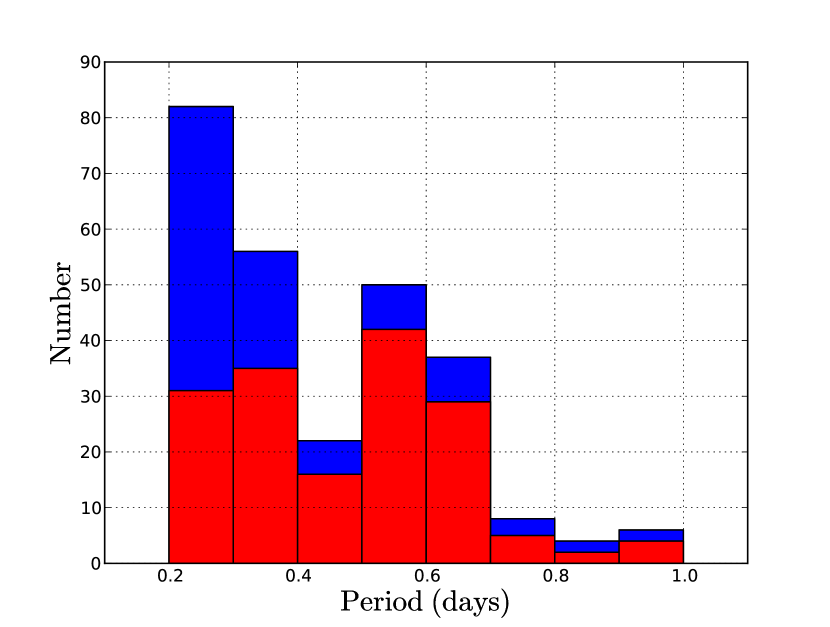
Figure 6.— Blue histogram: period distribution for 265 objects with at least 12 observations. Red histogram: period distribution for 170 bona fide RRLs.

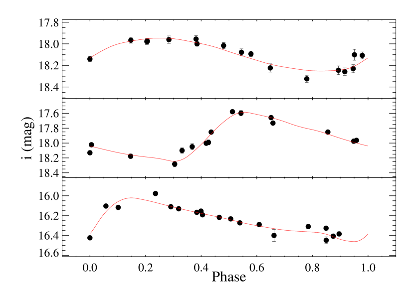
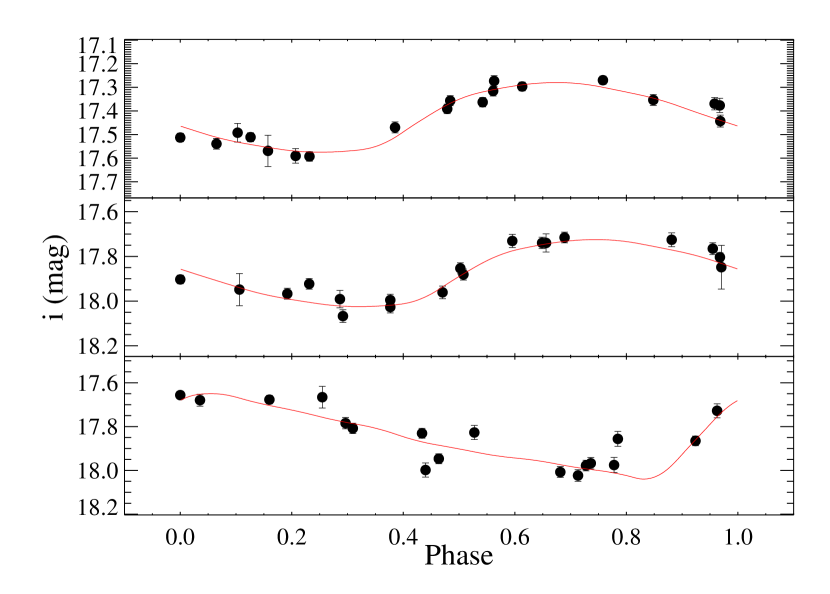
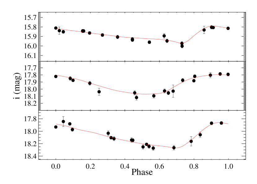
Figure 7.— Folded $i$ light-curves of selected RRL candidates.

6. Distance Estimation

Although there are period-luminosity relationships for RRLs (e.g. Cáceres & Catelan, 2008), we choose not to use them for our study because, as mentioned above, we do not have accurate periods for our entire sample. Therefore the best we can do is to attempt to estimate heliocentric distance $d_{\mathrm{h}}$ from their mean unreddened $i_{0}$ magnitude alone (the reddening correction is performed via the maps of Schlegel, Finkbeiner, & Davis, 1998) by comparing them to S10 unreddened absolute magnitudes, which we derived using the data they provide. We then calculate the S10 sample mean, which we use as our best estimate of $\langle I_{0}\rangle$ for RRLs in the galactic halo. After converting to the Xuyi system we find $\langle I_{0}\rangle=0.57~{}\mathrm{mag}$, with a dispersion of $0.08~{}\mathrm{mag}$. Note that by sampling the S10 absolute magnitude distribution we are effectively marginalizing over the periods; moreover, as S10 assume a mean halo metallicity [Fe/H]=-1.5 (from Ivezić et al., 2008) we are implicitly doing the same. Our distance indicator is thus given by the following equation:

$$d_{\mathrm{h}}=10^{(i_{0}-\langle I_{0}\rangle+5)/5)}/1000~{}\mathrm{kpc}.$$ (6)

We then construct an histogram of distances for our sample by correcting both for efficiency $\epsilon$ (described in Section 4) and for contamination $c$ (described in Section 5). We do this by assigning each RRL candidate a weight $w=(1-c)/\epsilon$ when constructing the histogram, with $c=0.36$; note that while $\epsilon$ varies from object to object, $c$ is the same for the whole sample. The result is shown in Figure 8, which also shows for comparison the histograms for the W09 and S10 samples, where, for these, we only included objects up to a galacto-centric distance $65~{}\mathrm{kpc}$ and did not perform any correction for efficiency or contamination (W09 explicitly state that $\epsilon\approx 1$ for their sample). The figure shows an excess RRL at $\approx 20~{}\mathrm{kpc}$ for the XSTPS sample and a smaller one at $\approx 35~{}\mathrm{kpc}$ for the W09 and S10 samples, in both cases exactly where the Sagittarius Stream is, so these excesses are probably due to contamination from stream stars; this is consistent with W09 who find that 55 RRLs in their sample are associated with the stream.

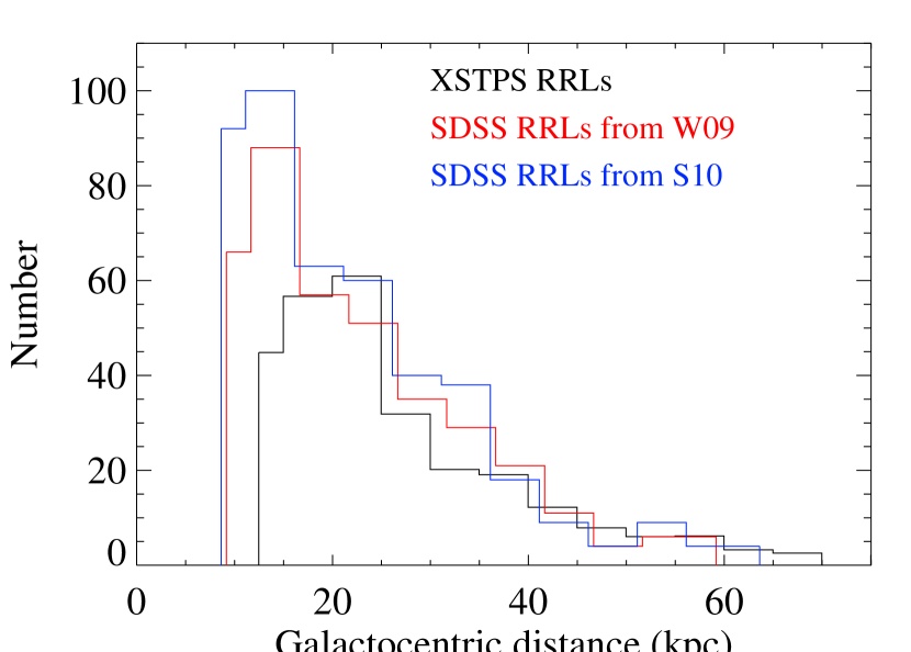
Figure 8.— Histogram of the galacto-centric distances for the XSTPS, W09, and S10 RRL samples; the XSTPS data are corrected for efficiency and contamination; only W09 and S10 RRLs with galacto-centric distances $<65~{}\mathrm{kpc}$ are shown.

We estimated our distance uncertainties using a MC process. For each candidate RRL we randomly sampled the distribution of absolute $I_{0}$ magnitudes from S10 (converted to the Xuyi photometric system). We did this 10,000 times and recomputed distances via Equation 6. The standard deviation of these resamples is then taken to represent the uncertainty in the distance. Typical MC uncertainties in the heliocentric distances are about $4\%$, which is entirely consistent with the expected uncertainties associated with the spread in $I_{0}$ (the relative uncertainty in distance $d$ is given by $\delta d/d=0.2\log(10)\delta\langle I_{0}\rangle=0.037$).

Since period-luminosity relationships are usually metallicity-dependent and we do not have metallicity information for our sample, this will add an uncertainty of 0.07 mag in $V$ (see section 4.1 of S10 for details of how this value is determined). Furthermore, as discussed in Vivas & Zinn (2006), the change in absolute magnitude with the RRL evolution off the Zero Age Horizontal Branch will affect the distance estimation, introducing an additional dispersion of $0.08~{}\mathrm{mag}$ in $V$. Even though both of these contributions should already be taken into account when we sample the S10 absolute magnitude distribution (since this will include RRL of various metallicities, consistent with the metallicity spread of the halo, and RRL in a variety of evolutionary states), we choose to be conservative and include them in our total error budget. Assuming that the spread in $V$ is similar to the spread in our Xuyi $i$-band for these two terms, this means that the total uncertainty in absolute magnitude is $\delta\langle I_{0}\rangle\approx\sqrt{0.08^{2}+0.07^{2}+0.08^{2}}=0.13$. When combined with the photometric uncertainties in $i_{0}$, which are typically around a few hundreths of a magnitude for our Xuyi sample, we find our distances are accurate to $\approx 6-7\%$, consistent with similar values found by S10 and Vivas & Zinn (2006). The distances and the uncertainties from the MC procedure are given in an accompanying electronic table.

It is now easy to derive the spatial distribution of RRLs in a galacto-centric reference frame $X_{\mathrm{GC}},Y_{\mathrm{GC}},Z_{\mathrm{GC}}$, which is shown in Figure 9 in the $R_{\mathrm{GC}}\equiv\sqrt{X_{\mathrm{GC}}^{2}+Y_{\mathrm{GC}}^{2}},Z_{\mathrm{GC}}$ plane; we assume a distance to the Galactic Center ($\mathrm{GC}$) of $8~{}\mathrm{kpc}$ and $Z_{\mathrm{GC}}$ is directed toward the North Galactic Pole; the figure shows all the RRLs in the sample, including the few that are beyond our magnitude limit $i=19~{}\mathrm{mag}$

Figure 9.— RRL distribution in the $R_{\mathrm{GC}}\equiv\sqrt{X_{\mathrm{GC}}^{2}+Y_{\mathrm{GC}}^{2}},Z_{\mathrm{GC}}$ plane.

7. The halo density profile

7.1. Spherical Halo Models

We now use our data to study the halo density profile in the NGC and compare the results to those obtained using the W09 and S10 samples for the SGC. Note that the W09 and S10 samples have been constructed using the same SDSS data and hence are not independent samples. We start by considering spherically symmetric models in the form $n=n(r)$ where $r$ is the galacto-centric distance.

The halo density profile out to the outer halo has often been parameterized as a double broken power law (see W09 for a discussion and, for a collection of recent results, Akhter et al., 2012); in particular W09 fit a double power law to their data-set in the form:

$$n(r)=n_{0}\begin{cases}\left(\frac{R_{0}}{r}\right)^{\alpha}&\text{if $R_{\mathrm{min}}<r<R_{0}$,}\\ \left(\frac{R_{0}}{r}\right)^{\beta}&\text{if $R_{0}<r<R_{\mathrm{max}}$}\end{cases}$$ (7)

and derive the following values for the halo parameters in the SGC: $(n_{0},R_{0},\alpha,\beta)=(0.26~{}\mathrm{kpc}^{-3},23~{}\mathrm{kpc},2.4,4.5)$ . We fit Equation 7 to the XSTPS, W09, and S10 data-sets. To fit Equation 7 we need to determine the completeness limit of the XSTPS, W09, and S10 data-sets and use this limit as $R_{\mathrm{max}}$. In Section 2 we used Figure 2 to argue that the completeness limit for finding RRLs in XSTPS is around $i=19~{}\mathrm{mag}$; beyond that limit the photometric uncertainties become too large to reliably identify RRLs by the variability cuts we employed. Assuming a mean absolute magnitude $\langle I_{0}\rangle=0.57~{}\mathrm{mag}$ (see Section 6) we derive via Equation 6 a maximum distance for our sample of $48.62~{}\mathrm{kpc}$; we therefore adopt a maximum distance, $R_{\mathrm{max}}=49~{}\mathrm{kpc}$ that allows us to sample the halo well past the broken power law regime (the break takes place at $R_{0}\approx 23~{}\mathrm{kpc}$, see W09). We use this same value of $R_{\mathrm{max}}$ for the W09 and S10 data for three reasons: first for consistency with our data, second because at higher distances the number of RRLs becomes so low that the quality of the fit may be affected (unlike W09 we fit for the density, not its volume integral), and finally because at higher distances the W09 and S10 samples are affected by local over-densities that may negatively impact a fit to a smooth profile (again this may be less of a concern for W09 who fit for the volume integral of the density); we also remove from the fit the few RRLs in all samples with distance $r<9~{}\mathrm{kpc}$. We compute the measured $n(r)$ to be fit to Equation 7 by binning the RRLs in $1~{}\mathrm{kpc}$ bins in the $9-49~{}\mathrm{kpc}$ range, assigning each candidate a weight $w=(1-0.36)/\epsilon$ where $0.36$ is the contamination computed in Section 5 and $\epsilon$ is the efficiency computed in Section 4, and dividing by the bin volume. Note that the bin volumes, being centered on the GC and not on the Sun, cannot be naively computed as $V=\frac{\Omega}{3}(R_{2}^{3}-R_{1}^{3})$ (where $\Omega=376.75~{}\mathrm{deg}^{2}$ is the XSTPS stripe area and $R_{1}$, $R_{2}$ are the bin boundaries) because the stripe area is valid for a helio-centric coordinates system. Therefore we computed them by numerical integration, generating random RRLs distributed in a large cubic volume around the GC and counting the fraction of these RRLs that would both fall within each radial bin and that would be visible in our stripe; this fraction, multiplied by the cubic volume, gives the bin volume; this is very important for RRLs whose galacto-centric distance is not much greater than our adopted Sun-GC distance ($8~{}\mathrm{kpc}$) but becomes less and less important for RRLs at greater distances. Uncertainties are estimated using Poisson statistics, dividing the square root of the weighted number of RRL candidates in each $1~{}\mathrm{kpc}$ bin by the bin volume. We do the same for the W09 and S10 data-sets, except that in that case we assign $w=1$ to each RRL since both samples are free of contamination and have $\epsilon\approx 1$ (Watkins et al., 2009; Sesar et al., 2010) due to their good light-curve sampling.

The fit results are summarized in Table 2.

Table 2Summary of fits to double power law (Equation 7).

Data	$n_{0}~{}(\mathrm{kpc}^{-3})$	$R_{0}~{}(\mathrm{kpc})$	$\alpha$	$\beta$	$\chi^{2}/\mathrm{dof}$
XSTPS	$0.42\pm 0.16$	$21.5\pm 2.2$	$2.3\pm 0.5$	$4.8\pm 0.5$	$0.65$
XSTPSa	$0.40\pm 0.19$	$21.5\pm 2.6$	$2.4\pm 0.5$	$4.7\pm 0.5$	$0.64$
W09	$0.28\pm 0.11$	$22.9\pm 2.5$	$2.8\pm 0.3$	$4.9\pm 0.5$	$1.22$
S10	$0.21\pm 0.08$	$25.5\pm 2.4$	$2.9\pm 0.3$	$5.2\pm 0.6$	$1.05$

This table shows that the three data-sets give results consistent with each other at the $\approx 1\sigma$ level (albeit with a rather large formal uncertainty) for all the halo profile parameters.

One concern that should be addressed is a possible contamination of our data by Sagittarius Stream stars in the XSTPS stripe area (see for example Figure 1 of Belokurov et al. 2006). Law & Majewski (2010) present a model of the Sagittarius Stream based on a triaxial Milky Way halo which reproduces most observational constraints and present the results of their $N-$body simulations in the form of three dimensional positions and velocities of 10,000 Sagittarius Stream particles both for the leading and the trailing arm of the stream; their results show that the distribution of particles is strongly peaked at $\approx 20~{}\mathrm{kpc}$ in the area covered by XSTPS data. Therefore we redid the fit removing the data with $19~{}\mathrm{kpc}<r<21~{}\mathrm{kpc}$. Results of this fit are given in the second row of Table 2 and, reassuringly, show very little variation from the original fit.

The W09 and S10 samples are also contaminated by Sagittarius Stream stars (W09). The Law & Majewski (2010) model shows that at the SDSS Stripe 82 location the star distribution peaks at $\approx 20$ and $40~{}\mathrm{kpc}$ but these peaks are much less sharp than the one exhibited by stream stars at the  XSTPS location; we checked that removing RRLs at those distances in the W09 and S10 samples does not affect the fit much so we did not correct for Sagittarius Stream contamination for the W09 and S10 samples. More detailed studies, for example folding in the velocities or chemistry of the stars, would be able to address the issue of Sagittarius contamination more robustly, but we do not wish to attempt such analyses here.

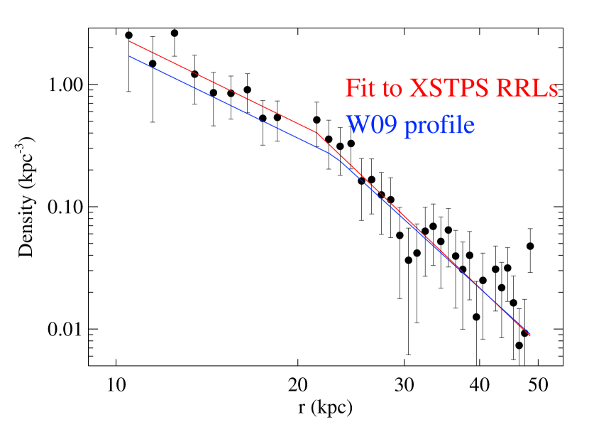
Figure 10.— RRL number density as a function of galacto-centric distance in the $9-49~{}\mathrm{kpc}$ range with the XSTPS RRLs at $\approx 20~{}\mathrm{kpc}$ removed from the fit to account for possible contamination from Sagittarius Stream stars. The red line shows the fit to a double power law given by Equation 7. The blue line shows the W09 profile with $n_{0}=0.26~{}\mathrm{kpc}^{-3}$.

Our halo profile fit is illustrated in Figure 10, which also shows the W09 profile with $n_{0}=0.26~{}\mathrm{kpc}^{-3}$. The agreement between the XSTPS and W09 sample is excellent, whereas from Table 2 we can see that the S10 sample is somewhat more discrepant; in all cases however we find evidence for a steepening of the halo density profile beyond $23-25~{}\mathrm{kpc}$, consistent with both W09 and S10.

Therefore we may conclude that the halo density profile in the NGC in the $9-49~{}\mathrm{kpc}$ range (as sampled by the RRLs in the XSTPS data-set) is in broad agreement with the density profile in the SGC in the same range (as sampled by the RRLs in the W09 and S10 data-sets). Both NGC and SGC data can be adequately described by a double power law given by Equation 7 with parameters consistent across all three data-sets at the $1\sigma$ level.

7.2. Non-spherical Halo Models

It is interesting to check whether our RRLs, as well as the W09 and S10 ones, can constrain non-spherical models of the halo as there is evidence that the halo density profile can be best described by oblate or triaxial models.

Deason, Belokurov, & Evans (2011, hereafter D11) use a maximum likelihood method to study the density profile of BHB and blue straggler stars from SDSS Data Release 8; their sample comprises $\approx 20,000$ stars over a $14,000~{}\mathrm{deg}^{2}$ area encompassing both the Northern and the Southern Galactic hemispheres; their main finding is that oblate and triaxial halo models describe their data better than spherical ones, with an oblate double power law model giving the highest likelihood overall. Sesar et al. (2011b, hereafter S11) use Canada-France-Hawaii Legacy Survey data in a $170~{}\mathrm{deg}^{2}$ area along four lines of sight to probe the galactic halo via the distribution of near-turnoff main-sequence stars up to an heliocentric distance of $\approx 35~{}\mathrm{kpc}$. S11 too find that the halo profile can best be described by an oblate double power law as well as detecting both the Sagittarius and the Monoceros Streams. Non-spherical halo models have also been considered by Vivas & Zinn (2006) who find that non-spherical single power law models better describe their RRL sample.

We reanalyzed the XSTPS, W09, and S10 data-sets in light of the D11 and S11 results: we started by setting up a cylindrical coordinate system with origin in the Galactic Center, described by $R_{\mathrm{GC}}\equiv\sqrt{X_{\mathrm{GC}}^{2}+Y_{\mathrm{GC}}^{2}}$, $\phi\equiv\arctan(Y_{\mathrm{GC}}/X_{\mathrm{GC}})$, and $Z_{\mathrm{GC}}$ where $X_{\mathrm{GC}},Y_{\mathrm{GC}},Z_{\mathrm{GC}}$ are galacto-centric coordinates and consider a non-spherical double power law model:

$$n(r_{q})=n_{0}\begin{cases}\left(\frac{R_{0}}{r_{q}}\right)^{\alpha}&\text{if $R_{\mathrm{min}}<r_{q}<R_{0}$},\\ \left(\frac{R_{0}}{r_{q}}\right)^{\beta}&\text{if $R_{0}<r_{q}<R_{\mathrm{max}}$}\end{cases}$$ (8)

where $r_{q}\equiv\sqrt{R_{\mathrm{GC}}^{2}+Z_{\mathrm{GC}}^{2}q^{-2}}$ and $q$ is a new parameter describing the flattening of the halo: $q<1$ for oblate models, $q>1$ for prolate models and $q=1$ for spherical ones, in which case Equation 8 reduces to Equation 7; the meaning of the other symbols is the same as Equation 7. D11 find that a model described by Equation 8 with parameters $R_{0}=27\pm 1~{}\mathrm{kpc}$, $\alpha=2.3\pm 0.1$, $\beta=4.6^{+0.2}_{-0.1}$, and $q=0.59^{+0.02}_{-0.03}$, best fit their data; note that since they are analyzing different stellar tracers (BHBs and blue stragglers, rather than RRLs), we are not concerned with their value for the normalization. First we considered the D11 results, fitting Equation 8 assuming $q=0.59$; as usual we considered RRLs with a galacto-centric distance $9~{}\mathrm{kpc}<r<49~{}\mathrm{kpc}$ for all three data-sets and binned them in $1~{}\mathrm{kpc}$ bins as we did for the spherical cases; we also removed again RRLs with $19~{}\mathrm{kpc}<r<21~{}\mathrm{kpc}$ in the XSTPS data-set to avoid contamination from stars in the Sagittarius Stream. Figure 11 shows the density profile $n(r_{q})$ for the XSTPS data and the fit to Equation 8 with the parameters given by Table 3; also shown is the D11 profile with $n_{0}=0.38~{}\mathrm{kpc}^{-3}$ from our fit. Note that, even though we cut at $r=49~{}\mathrm{kpc}$, $r_{q}$ can reach much higher values since the $Z$ component of $r_{q}$ is divided by $q^{2}=0.348$

Table 3Summary of fits to oblate double power law (Equation 8 with $q=0.59$) with the XSTPS RRLs at $\approx 20~{}\mathrm{kpc}$ removed from the fit to account for possible contamination from Sagittarius Stream stars. The D11 results are taken from Deason, Belokurov, & Evans (2011).

Data	$n_{0}~{}(\mathrm{kpc}^{-3})$	$R_{0}~{}(\mathrm{kpc})$	$\alpha$	$\beta$	$\chi^{2}/\mathrm{dof}$
XSTPS	$0.31\pm 0.33$	$26.5\pm 8.9$	$2.7\pm 0.6$	$3.6\pm 0.4$	$1.04$
W09	$0.43\pm 0.16$	$26.9\pm 3.1$	$2.1\pm 0.3$	$4.0\pm 0.3$	$0.69$
S10	$0.42\pm 0.40$	$26.2\pm 7.4$	$3.0\pm 0.3$	$3.8\pm 0.3$	$1.52$
D11	N.A.	$27\pm 1$	$2.3\pm 0.1$	$4.6^{+0.2}_{-0.1}$	N.A.

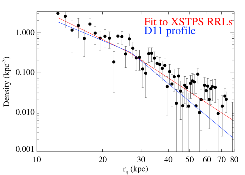
Figure 11.— RRL number density as a function of $r_{q}$ in the galacto-centric distance $r=9-49~{}\mathrm{kpc}$ range with the XSTPS RRLs at $\approx 20~{}\mathrm{kpc}$ removed from the fit to account for possible contamination from Sagittarius Stream stars. The red line shows the fit to a double power law given by Equation 8 with $q=0.59$. The blue line shows the D11 profile with $n_{0}=0.31~{}\mathrm{kpc}^{-3}$ from our fit (see Table 3).

Table 3 shows that agreement with the D11 result is excellent for all three RRL data-sets for the break radius $R_{0}$ and at about $1\sigma$ level for $\alpha$, while there is some tension (at about $2\sigma$ level) for $\beta$ with the RRL data preferring lower values. It should be noted however that the formal errors from the fits are considerable (for example, for the XSTPS  and S10 samples the error on $n_{0}$ is of the same magnitude as $n_{0}$ itself) and the $\chi^{2}/\mathrm{dof}$ is rather large for the S10 sample, suggesting that these current RRL data-sets are unable to provide strong constraints on this model. Of the three RRL samples we considered, W09 is both the one that is better described by an oblate halo model with $q=0.59$ and the one for which the agreement with the D11 result is best.

We then considered the S11 results, which differ quite considerably from those of D11 (this may be due to the fact that the two groups use different tracer populations, with D11 using BHB and Blue Straggler stars while S11 use near-turnoff main-sequence stars). While the agreement for the break radius $R_{0}$ is excellent, there is tension at the few $\sigma$ level for $\alpha$ and $\beta$; S11 also find evidence for a less oblate halo ($q=0.70\pm 0.01$).

Table 4Summary of fits to oblate double power law (Equation 8 with $q=0.7$) with the XSTPS RRLs at $\approx 20~{}\mathrm{kpc}$ removed from the fit to account for possible contamination from Sagittarius Stream stars. The S11 results are taken from Sesar et al. (2011b); the $n_{0}$ parameter refers to near-turnoff main-sequence stars so it cannot be compared to the RRL values.

Data	$n_{0}~{}(\mathrm{kpc}^{-3})$	$R_{0}~{}(\mathrm{kpc})$	$\alpha$	$\beta$	$\chi^{2}/\mathrm{dof}$
XSTPS	$0.21\pm 0.14$	$28.5\pm 5.6$	$2.8\pm 0.4$	$4.4\pm 0.7$	$0.8$
W09	$0.28\pm 0.12$	$27.6\pm 3.3$	$2.5\pm 0.3$	$4.3\pm 0.4$	$1.1$
S10	$0.15\pm 0.04$	$34.6\pm 2.8$	$2.8\pm 0.2$	$5.8\pm 0.9$	$1.1$
S11	$1450\pm 50$	$27.8\pm 0.8$	$2.62\pm 0.04$	$3.8\pm 0.1$	$3.9$

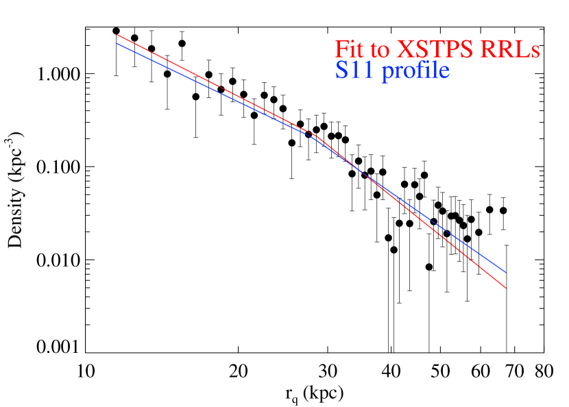
Figure 12.— RRL number density as a function of $r_{q}$ in the galacto-centric distance $r=9-49~{}\mathrm{kpc}$ range with the XSTPS RRLs at $\approx 20~{}\mathrm{kpc}$ removed from the fit to account for possible contamination from Sagittarius Stream stars. The red line shows the fit to a double power law given by Equation 8 with $q=0.7$. The blue line shows the S11 profile with $n_{0}=0.32~{}\mathrm{kpc}^{-3}$ from our fit (see Table 4).

Our results using this S11 flattening are presented in Figure 12, which shows the density profile $n(r_{q})$ for the XSTPS data and the fit to Equation 8, with the parameters given in Table 4; also shown is the S11 profile normalized to match our fit. Table 4 shows good agreement in $R_{0}$, $\alpha$ and $\beta$ between XSTPS, W09 and S11, although there is some tension with S10. It should be noted that again the formal uncertainties are rather large. The $\chi^{2}/\mathrm{dof}$ are somewhat lower than the $q=0.59$ case for XSTPS and S10 (but higher for W09), suggesting that current RRL data prefer a less oblate halo than D11 and agree more with S11. It should be emphasized however that the fact that the three RRL samples provide a decent fit to both spherical and oblate halo models shows that they are not able to provide strong constraints for non-spherical halo models and that larger samples with greater sky coverage are needed. Wide-field surveys are beginning to make this possible, for example the work of Sesar et al. (2013) who use RRL from LINEAR to measure a halo flattening of $0.63\pm 0.05$.

We finally note that Akhter et al. (2012) present a compilation of recent studies that modelled the halo as a double power law using both a variety of data-sets and a variety of tracers and considering both spherical and non-spherical models. These studies find a great variety of values for the break radius, ranging from $23$ kpc (W09) to $45$ kpc (Keller et al., 2008); the inner power law index $\alpha$ is much better constrained, with values mostly in the $2.3-2.7$ range; the outer power law index $\beta$ is less well constrained with values ranging from $3.6$ to $5$; of all these studies we find the best agreement with W09 but clearly more work is needed as the spread in values found by the different studies, especially for the break radius, is still very large.

8. Conclusions

We have presented a sample of 318 candidates RRLs observed by the XSTPS in an $\approx 376.75~{}\mathrm{deg}^{2}$ stripe in the NGC, selected via a combination of SDSS color cuts and variability information afforded by the multi-epoch nature of these XSTPS observations. We have quantified the efficiency of our discovery procedure via Monte Carlo methods and, by estimating the period for those candidate RRLs that have enough observations, we have also quantified the effect of contamination from non-RRL passing our color and variability cuts. We have estimated a distance to the RRLs by assuming a mean absolute magnitude and have used this information to probe the halo density profile in the NGC in the $9-49~{}\mathrm{kpc}$ range. We found that the halo can be well approximated by a double power law, as found in the SGC by W09. There is agreement at the $1\sigma$ level between our model and the models derived for the SGC using the W09 and S10 data-sets, and, after removing RRLs at $r\approx 20~{}\mathrm{kpc}$ in our sample from the fit to account for possible contamination from RRLs in the Sagittarius Stream, the agreement between our sample and the SGC samples further improves; in particular the agreement with the W09 result is excellent. We considered non-spherical double power law models of the halo density profile and found again agreement between the results from our sample, the W09 and S10, and two samples using different halo tracers: the D11 BHB and Blue Stragglers sample and the S11 near-turnoff main-sequence stars. Our fits show that the XSTPS and S10 samples favor the less oblate halo model of S11, whereas the W09 samples agree with the more oblate model of D11. However, the fits are affected by large formal uncertainties and, when comparing to D11, mediocre goodness of fit (at least for the S10 sample). Furthermore there could be population effects since these different studies use a variety of halo tracer populations. We therefore conclude that these RRL samples are not able to provide strong constraints for non-spherical halo models and that larger samples with greater sky coverage are needed. This is already being made possible by projects such as LINEAR (Sesar et al., 2013), the Catalina Survey (Drake et al., 2013a), the Palomar Transient Factory (Rau et al., 2009) and Pan-STARRS (Kaiser et al., 2002). In the near future Gaia, ESA’s space astrometry mission, will map the entire sky repeatedly down to 20th magnitude (de Bruijne, 2012), becoming a valuable resource for RRLs and other standard candles (Bono, 2003b; Eyer et al., 2012). Although most of the sky will be monitored with an average of 70 epochs, certain regions will only have a few tens of measurements (see figure 3 of de Bruijne, 2012). However, as we have shown in this paper, even with a limited number of epochs it is still possible to catalog and analyze the properties of RRLs. The coming decade will provide unprecedented samples of RRLs, which will be an invaluable resource for understanding the profile of our stellar halo and illuminating the nature of the dark matter distribution around our galaxy.

References

- Akhter et al. (2012) Akhter S., Da Costa G. S., Keller S. C., Schmidt B. P., 2012, ApJ, 756, 23
- Alcock et al. (1993) Alcock C., et al., 1993, Natur, 365, 621
- Alcock et al. (1998) Alcock C., et al., 1998, ApJ, 492, 190
- Aubourg et al. (1993) Aubourg E., et al., 1993, Natur, 365, 623
- Belokurov et al. (2006) Belokurov V., et al., 2006, ApJ, 642, L137
- Bond et al. (2010) Bond N. A., et al., 2010, ApJ, 716, 1
- Bono (2003a) Bono G., 2003a, in Alloin D., Gieren W., eds, Lecture Notes in Physics, Vol. 635, Stellar Candles for the Extragalactic Distance Scale, p. 85
- Bono (2003b) Bono G., 2003b, in Munari U., ed, ASP Conference Proceedings, Vol. 298, GAIA Spectroscopy: Science and Technology, p. 245
- Bowell et al. (1995) Bowell E., Koehn B. W., Howell S. B., Hoffman M., Muinonen K., 1995, DPS, 27, 1057
- Bramich et al. (2008) Bramich D. M., et al., 2008, MNRAS, 386, 887
- de Bruijne (2012) de Bruijne J.H.J., 2012, Astrophys Space Sci, 341, 31
- Cáceres & Catelan (2008) Cáceres C., Catelan M., 2008, ApJS, 179, 242