The Use of a Single Pseudo-Sample
in Approximate Bayesian Computation

Abstract

We analyze the computational efficiency of approximate Bayesian computation (ABC), which approximates a likelihood function by drawing pseudo-samples from the associated model. For the rejection sampling version of ABC, it is known that multiple pseudo-samples cannot substantially increase (and can substantially decrease) the efficiency of the algorithm as compared to employing a high-variance estimate based on a single pseudo-sample. We show that this conclusion also holds for a Markov chain Monte Carlo version of ABC, implying that it is unnecessary to tune the number of pseudo-samples used in ABC-MCMC. This conclusion is in contrast to particle MCMC methods, for which increasing the number of particles can provide large gains in computational efficiency.

1 Introduction

Approximate Bayesian computation (ABC) is a family of algorithms for Bayesian inference that address situations where the likelihood function is intractable to evaluate but where one can obtain samples from the model. These methods are now widely used in population genetics, systems biology, ecology, and other areas, and are implemented in an array of popular software packages (tavare1997inferring; marin2012approximate). Let $\bm{\theta}\in\Theta$ be the parameter of interest with prior density $\pi(\bm{\theta})$, $\bm{y}_{\mathrm{obs}}\in\mathcal{Y}$ be the observed data and $p(\bm{y}|\bm{\theta})$ be the model. The simplest ABC algorithm first generates a sample $\bm{\theta^{\prime}}\sim\pi(\bm{\theta})$ from the prior, then generates a pseudo-sample $\bm{y}_{\bm{\theta}^{\prime}}\sim p(\cdot|\bm{\theta}^{\prime})$. Conditional on $\bm{y}_{\bm{\theta}^{\prime}}=\bm{y}_{\mathrm{obs}}$, the distribution of $\bm{\theta^{\prime}}$ is the posterior distribution $\pi(\bm{\theta}|\bm{y}_{\mathrm{obs}})\propto\pi(\bm{\theta})p(\bm{y}_{\mathrm{obs}}|\bm{\theta})$. For all but the most trivial discrete problems, the probability that $\bm{y}_{\bm{\theta}^{\prime}}=\bm{y}_{\mathrm{obs}}$ is either zero or very small. Thus the condition of exact matching of pseudo-data to the observed data is typically relaxed to $\|\eta(\bm{y}_{\mathrm{obs}})-\eta(\bm{y}_{\bm{\theta}^{\prime}})\|<\epsilon,$ where $\eta$ is a low-dimensional summary statistic, $\|\cdot\|$ is a distance function, and $\epsilon>0$ is a tolerance level. The resulting algorithm gives samples from the target density $\pi_{\epsilon}$ that is proportional to $\left[\pi(\bm{\theta})\int\mathbf{1}_{\{\|\eta(\bm{y}_{\mathrm{obs}})-\eta(\bm{y})\|<\epsilon\}}p(\bm{y}|\bm{\theta})d\bm{y}\right]$. If the tolerance $\epsilon$ is small enough and the statistic(s) $\eta$ good enough, then $\pi_{\epsilon}$ can be a good approximation to $\pi(\bm{\theta}|\bm{y}_{\mathrm{obs}})$.

A generalized version of this method (wilk:08) is given in Algorithm 1, where $K(\eta)$ is an unnormalized probability density function, $M$ is an arbitrary number of pseudo-samples, and $c$ is a constant satisfying $c\geq\sup_{\eta}K(\eta)$.

for $t=1$ to $n$ do

       repeat

             Generate $\bm{\theta}^{\prime}\sim\pi(\bm{\theta})$, $\bm{y}_{i,\bm{\theta}^{\prime}}\stackrel{{\scriptstyle\mbox{\tiny iid}}}{{\sim}}p(\bm{y}|\bm{\theta}^{\prime})$ for $i=1,\dots,M$, and $u\sim\mbox{Uniform}[0,1]$.

      until $u<\frac{1}{cM}\sum_{i=1}^{M}K(\eta(\bm{y}_{\mathrm{obs}})-\eta(\bm{y}_{i,\bm{\theta}^{\prime}}))$;

      Set $\bm{\theta}^{(t)}=\bm{\theta}^{\prime}$;

      

Algorithm 1 Generalized ABC

Using the “uniform kernel” $K(\eta)=\mathbf{1}_{\{\|\eta\|<\epsilon\}}$ and taking $M=c=1$ yields the version described above. Algorithm 1 yields samples $\bm{\theta}^{(t)}$ from the kernel-smoothed posterior density π_K(θ— y_obs) ∝π(θ) ∫K( η(y_obs)- η(y) )  p(y—θ)  dy. Although Algorithm 1 is nearly always presented in the special case with $M=1$ (wilk:08), it is easily verified that $M>1$ still yields samples from $\pi_{K}(\bm{\theta}|\bm{y}_{\mathrm{obs}})$.

Many variants of Algorithm 1 exist. For any unbiased, nonnegative estimator $\hat{\mu}(\bm{\theta})$ of $\pi_{K}(\bm{\theta}|\bm{y}_{\mathrm{obs}})$ and any reversible transition kernel $q$ on $\Theta$, Algorithm 2 gives a Markov chain Monte Carlo (MCMC) version that is based on the pseudo-marginal algorithm of (andrieu2009the-pseudo-marginal) (see also (marj:03; wilk:08; Andrieu2014establishing-some-order)). To obtain an algorithm that is similar to Algorithm 1, a good choice for $\hat{\mu}(\bm{\theta})$ is ^π_K,M(θ— y_obs) ≡π(θ)1 M ∑_i=1^M K(η(y_obs) - η(y_i,θ)), where $M\in\mathbb{N}$. When we refer to Algorithm 2, we always use this family of weights unless stated otherwise. Despite the fact that the expression (1) depends on $M$, as $n\rightarrow\infty$ the distribution of $x^{(n)}$ in Algorithm 2 converges to the same distribution $\pi_{K}$ under mild conditions (Andrieu2014establishing-some-order). Although the choice of $M$ in (1) generally does not affect the limiting distribution of $x^{(n)}$, it does affect the evolution of the stochastic process $\{x^{(n)}\}_{n\in\mathbb{N}}$.

Initialize $x^{(0)}$ and generate $T^{(0)}=\hat{\mu}(x^{(0)})$;

for $t=1$ to $n$ do

       Generate $x^{\prime}\sim q(\cdot|x^{(t-1)})$, $T^{\prime}=\hat{\mu}(x^{\prime})$, and $u\sim\mbox{Uniform}[0,1]$;

       if $u\leq\frac{T^{\prime}q(x^{(t-1)}|x^{\prime})}{T^{(t-1)}q(x^{\prime}|x^{(t-1)})}$ then

             Set $\left(x^{(t)},T^{(t)}\right)$ = $\left(x^{\prime},T^{\prime}\right)$;

            

      else

             Set $\left(x^{(t)},T^{(t)}\right)$ = $\left(x^{(t-1)},T^{(t-1)}\right)$;

            

Algorithm 2 Pseudo-Marginal MCMC

We address the effect of $M$ on the efficiency of Algorithm 2 when using the weight (1). Increasing the number of pseudo-samples $M$ decreases the variance of 2, which one might think could improve the efficiency of Algorithm 2. Indeed, increasing $M$ does decrease the asymptotic variance of the associated Monte Carlo estimates (Andrieu2014establishing-some-order). However, increasing $M$ also increases the computational cost of each step of the algorithm. Although the tradeoff between these two factors is quite complicated, our main result in this paper gives a good compromise: the choice $M=1$ yields a running time within a factor of two of optimal. We use natural definitions of running time in the contexts of serial and parallel computing, which are extensions of those used by pitt2012on-some, sherlock2013on-the-efficiency, and Doucet2014efficient-implementation, and which capture the time required to obtain a particular Monte Carlo accuracy. Our definition in the serial computing case is the number of pseudo-samples generated, which is an appropriate measure of running time when drawing pseudo-samples is more computationally intensive than the other steps in Algorithm 2, and when the expected computational cost of drawing each pseudo-sample is the same, i.e. when there is no computational discounting due to having pre-computed relevant quantities.

Several authors have drawn the conclusion that in many situations the approximately optimal value of $M$ in pseudo-marginal algorithms (a class of algorithms that includes Algorithm 2) is obtained by tuning $M$ to achieve a particular variance for the estimator $\hat{\pi}_{K,M}(\bm{\theta}|\bm{y}_{\mathrm{obs}})$ (pitt2012on-some; sherlock2013on-the-efficiency; Doucet2014efficient-implementation). This often means a value of $M$ that is much larger than 1. We demonstrate that in Algorithm 2 such a tuning process is unnecessary, since near-optimal efficiency is obtained by using estimates based on a single pseudo-sample (Proposition 4 and Corollary 5); these estimates are lower-cost and higher-variance than those based on several pseudo-samples. This result assumes only that the kernel $K(\eta)$ is the uniform kernel $\mathbf{1}_{\{\|\eta\|<\epsilon\}}$ (the most common choice). In particular, and in contrast to earlier work, it does not make any assumptions about the target distribution $\pi(\bm{\theta}|\bm{y}_{\mathrm{obs}})$.

Our result is in contrast to particle MCMC methods (andrieu2010particle), which flury2011bayesian demonstrated could require thousands, millions or more particles to obtain sufficient accuracy in some realistic problems. This difference between particle MCMC and ABC-MCMC is largely due to the interacting nature of the particles in particle MCMC, allowing for better path samples.

2 Efficiency of ABC and ABC-MCMC

For a measure $\mu$ on space $\mathcal{X}$ let $\mu(f)\equiv\int f(x)\mu(dx)$ be the expectation of a real-valued function $f$ with respect to $\mu$ and let $L^{2}(\mu)=\{f:\mu(f^{2})<\infty\}$ be the space of functions with finite variance. For any reversible Markov transition kernel $H$ with stationary distribution $\mu$, any function $f\in L^{2}(\mu)$, and Markov chain $X^{(t)}$ evolving according to $H$, the MCMC estimator of $\mu(f)$ is $\bar{f}_{n}\equiv\frac{1}{n}\sum_{t=1}^{n}f(X^{(t)})$. The error of this estimator can be measured by the asymptotic variance: v(f,H) = lim_n →∞ n Var_H ( ¯f_n ) which is closely related to the autocorrelation of the samples $f(X^{(t)})$ (tierney1998ordering).

If $H$ is geometrically ergodic, $v(f,H)$ is guaranteed to be finite for all $f\in L^{2}(\mu)$, while in the non-geometrically ergodic case $v(f,H)$ may or may not be finite (robe:rose:08). When $v(f,H)$ is infinite our results still hold but are not informative. The fact that our results do not require geometric ergodicity distinguishes them from many results on efficiency of MCMC methods (guan:kron:07; wood:schm:hube:09a). When $X^{(t)}\stackrel{{\scriptstyle\mbox{\tiny iid}}}{{\sim}}\mu$, we define $v(f)=\mathrm{Var}\left(f(X^{(t)})\right)$.

We will describe the running time of Algorithms 1 and 2 in two cases: first, when the computations are done serially, and second, when they are done in parallel across $M$ processors. Using (2), the variance of $\bar{f}_{n}$ from a single (reversible) Markov chain $H$ of length $n$ is roughly $v(f,H)/n$, so to achieve variance $\delta>0$ in the serial context we need $v(f,H)/\delta$ iterations. Similarly, the variance of $\bar{f}_{n}$ from a collection of $M$ reversible Markov chains, each run for $n$ steps, is roughly $v(f,H)/(Mn)$. Thus, to achieve variance $\delta>0$ in the parallel context we need to run each Markov chain for $n>v(f,H)/(\delta M)$ iterations.

Although our definitions make sense for any function $f$ of the two values $(\bm{\theta}^{(t)},T^{(t)})$ described by Algorithm 2, throughout the rest of the note we restrict our attention to functions that depend only on the first coordinate, $\bm{\theta}^{(t)}$. That is, when discussing Algorithm 2 or other pseudo-marginal algorithms, we restrict our attention to functions that satisfy $f(\bm{\theta},T_{1})=f(\bm{\theta},T_{2})$ for all $\bm{\theta}$ and all $T_{1},T_{2}$. We slightly abuse this in our notation, not distinguishing between a function $f:\Theta\mapsto\mathbb{R}$ of a single variable $\bm{\theta}$ and a function $f:\Theta\times\mathbb{R}^{+}\mapsto\mathbb{R}$ of two variables $(\bm{\theta},T)$ that only depends on the first coordinate.

Let $Q_{M}$ be the transition kernel of Algorithm 2; like all pseudo-marginal algorithms, $Q_{M}$ is reversible (andrieu2009the-pseudo-marginal). We assume that drawing pseudo-samples is the slowest part of the computation, and that drawing each pseudo-sample takes the same amount of time on average (as also assumed in Pitt et al. 2012, Sherlock et al. 2013, Doucet et al. 2014). Then the running time of $Q_{M}$ in the serial context can be measured as the number of iterations times the number of pseudo-samples drawn in each iteration, namely $C_{f,Q_{M},\delta}^{\mbox{\tiny ser}}\equiv Mv(f,Q_{M})/\delta$. In the context of parallel computation across $M$ processors, we compare two competing approaches that utilize all the processors. These are: (a) a single chain with transition kernel $Q_{M}$, where the $M>1$ pseudo-samples in each iteration are drawn independently across $M$ processors; and (b) $M$ parallel chains with transition kernel $Q_{1}$. The running time of these methods can be measured as the number of required Markov chain iterations to obtain accuracy $\delta$, namely $C_{f,Q_{M},\delta}^{\mbox{\tiny M-par}}\equiv v(f,Q_{M})/\delta$ utilizing method (a) and $C_{f,Q_{1},\delta}^{\mbox{\tiny M-par}}\equiv v(f,Q_{1})/(\delta M)$ utilizing method (b). Since both measures of computation time are based on the asymptotic variance of the underlying Markov chain, they ignore the initial ‘burn-in’ period and are most appropriate when the desired error $\delta$ is small. Other measures of computation time should be used if the Markov chains are being used to get only a very rough picture of the posterior (e.g. to locate, but not explore, a single posterior mode). Note, however, that in practice there is typically no burn-in period for Algorithm 2, since it is usually initialized using samples from ABC (marin2012approximate).

For Algorithm 1 the running time, denoted by $R_{M}$, is defined analogously. However, we must account for the fact that each iteration of $R_{M}$ yields one accepted value of $\bm{\theta}$, which may require multiple proposed values of $\bm{\theta}$ (along with the associated computations, including drawing pseudo-samples). The number of proposed values of $\bm{\theta}$ to get one acceptance has a geometric distribution with mean equal to the inverse of the marginal probability $p_{acc}(R_{M})$ of accepting a proposed value of $\bm{\theta}$. So, similarly to $Q_{M}$, the running time of $R_{M}$ in the context of serial computing can be measured as $C_{f,R_{M},\delta}^{\mbox{\tiny ser}}\equiv Mv(f)/(\delta\,p_{acc}(R_{M}))$, and the computation time in the context of parallel computing can be measured as $C_{f,R_{M},\delta}^{\mbox{\tiny M-par}}\equiv v(f)/(\delta\,p_{acc}(R_{M}))$ utilizing method (a) and $C_{f,R_{1},\delta}^{\mbox{\tiny M-par}}\equiv v(f)/(\delta Mp_{acc}(R_{1}))$ utilizing method (b).

Using these definitions, we first state the result that $M=1$ is optimal for ABC (Algorithm 1). This result is widely known but we could not locate it in print, so we include it here for completeness.

Lemma 1.

The marginal acceptance probability of ABC (Algorithm 1) does not depend on $M$. For $M>1$ the running times $C_{f,R_{M},\delta}^{\mbox{\tiny ser}}$ and $C_{f,R_{M},\delta}^{\mbox{\tiny M-par}}$ of ABC in the serial and parallel contexts satisfy $C_{f,R_{M},\delta}^{\mbox{\tiny ser}}=MC_{f,R_{1},\delta}^{\mbox{\tiny ser}}$ and $C_{f,R_{M},\delta}^{\mbox{\tiny M-par}}=MC_{f,R_{1},\delta}^{\mbox{\tiny M-par}}$ for any $f\in L^{2}(\pi_{K})$ and any $\delta>0$.

Proof.

The marginal acceptance probability of Algorithm 1 is

$$\int\pi(\bm{\theta})\left[\prod_{i=1}^{M}p(\bm{y}_{i,\bm{\theta}}|\bm{\theta})\right]\left[\frac{1}{cM}\sum_{i=1}^{M}K(\eta(\bm{y}_{\mathrm{obs}})-\eta(\bm{y}_{i,\bm{\theta}}))\right]\,d\bm{\theta}\,d\bm{y}_{1,\bm{\theta}}\ldots d\bm{y}_{M,\bm{\theta}}$$

$$=\frac{1}{c}\int\pi(\bm{\theta})p(\bm{y}|\bm{\theta})K(\eta(\bm{y}_{\mathrm{obs}})-\eta(\bm{y}))\,d\bm{\theta}\,d\bm{y}$$

which does not depend on $M$. The results for the running times follow immediately. ∎

Our contribution is to show a similar result for ABC-MCMC. A potential concern regarding Algorithm 2 is raised by lee2013ergodicity, who point out that this algorithm is generally not geometrically ergodic when $q$ is a local proposal distribution, such as a random walk proposal. This is due to the fact that in the tails of the distribution $\pi_{K}$, the pseudo-data $y_{i,\bm{\theta}}$ are very different from $y_{\mathrm{obs}}$ and so the proposed moves are rarely accepted. This problem can be fixed in several ways. Lee and Latuszynski (2013) give a sophisticated solution that involves choosing a random number of pseudo-samples at every step of Algorithm 2, and they show that this modification increases the class of target distributions for which the ABC-MCMC algorithm is geometrically ergodic. One consequence of our Proposition 4 is that a simpler ‘obvious’ fix to the problem of geometric ergodicity does not work: increasing the number of pseudo-samples used in Algorithm 2 from 1 to any fixed number $M$ has no impact on the geometric ergodicity of the algorithm.

Our main tool in analyzing Algorithm 2 will be the results of Andrieu2014establishing-some-order. Two random variables $X$ and $Y$ are convex ordered if $\mathbb{E}[\phi(X)]\leq\mathbb{E}[\phi(Y)]$ for any convex function $\phi$; we denote this relation by $X\leq_{cx}Y$. Let $H_{1},H_{2}$ be the transition kernels of two pseudo-marginal algorithms with the same proposal kernel $q$ and the same target marginal distribution $\mu$. Denote by $T_{1,x}$ and $T_{2,x}$ the estimators of the unnormalized target used by $H_{1}$ and $H_{2}$ respectively. Recall the asymptotic variance $v(f,H)$ from (2); although $f$ could be a function on $\mathcal{X}\times\mathbb{R}^{+}$, we restrict our attention to functions $f$ on the non-augmented state space $\mathcal{X}$. Then if $T_{1,x}\leq_{cx}T_{2,x}$ for all $x$, Theorem 3 of Andrieu2014establishing-some-order shows that $v(f,H_{1})\leq v(f,H_{2})$ for all $f\in L^{2}(\mu)$. As shown in Section 6 of that work, this tool can be used to show that increasing $M$ decreases the asymptotic variance of Algorithm 2:

Corollary 2.

For any $f\in L^{2}(\pi_{K})$ and any $M\leq N\in\mathbb{N}$ we have $v(f,Q_{M})\geq v(f,Q_{N}).$

In the appendix we give a similar comparison result for the alternative version of ABC-MCMC described in wilk:08.

We will show that, despite Corollary 2, it is not generally an advantage to use a large value of $M$ in Algorithm 2. To do this, we first give a result that follows easily from Theorem 3 of Andrieu2014establishing-some-order. For any $0\leq\alpha<1$ and $i\in\{1,2\}$, define the estimator T_i,x,α = {0 with  probability  αTi,x/(1 - α) otherwise. $T_{i,x,\alpha}$ has the same mean as $T_{i,x}$, but is a worse estimator. In particular, Proposition 1.2 of Lekela2014conditional-convex implies $T_{i,x}\leq_{cx}T_{i,x,\alpha}$ for any $0\leq\alpha\leq 1$ and any $i\in\{1,2\}$ (Equation (2) gives the coupling required by that proposition). We have:

Theorem 3.

Assume that $H_{2}$ is nonnegative definite. For any $0\leq\alpha<1$, if $T_{1,x}\leq_{cx}T_{2,x,\alpha}$ for all $x$, then for any $f\in L^{2}(\mu)$ we have v(f, H_1) ≤1+α1-α v( f, H_2).

Theorem 3 is proven in the appendix. The assumption that $H_{2}$ is nonnegative definite is a common technical assumption in analyses of the efficiency of Markov chains (wood:schm:hube:09a; nara:rakh:10), and is done here so we can compare $v(f,H_{2})$ to $v(f)$. It can easily be achieved, for example, by incorporating a “holding probability” (chance of proposing to stay in the same location) of 1/2 into the proposal kernel $q$ (wood:schm:hube:09a).

Theorem 3 yields the following bound for Algorithm 2, proven in the appendix.

Proposition 4.

If $K(\eta)=\textbf{1}_{\{\|\eta\|<\epsilon\}}$ for some $\epsilon>0$, and if the transition kernel $Q_{M}$ of Algorithm 2 is nonnegative definite, then for any $f\in L^{2}(\pi_{K})$ we have v(f, Q_1) ≤(2 M - 1) v(f, Q_M).

This yields the following bounds on the running times:

Corollary 5.

Using the uniform kernel and assuming that $Q_{M}$ is nonnegative definite, the running time of $Q_{1}$ is at most twice that of $Q_{M}$, for both serial and parallel computing:

$$C_{f,Q_{1},\delta}^{\mbox{\tiny ser}}\leq 2C_{f,Q_{M},\delta}^{\mbox{\tiny ser}}\qquad\mbox{and}\qquad C_{f,Q_{1},\delta}^{\mbox{\tiny M-par}}\leq 2C_{f,Q_{M},\delta}^{\mbox{\tiny M-par}}.$$

Corollary 5 implies that, under the condition that a uniform kernel is being used and that all pseudosamples have the same computational cost, it is only possible to improve the running time of the Markov chain by a factor of 2 by choosing $Q_{M}$ rather than $Q_{1}$. Thus, under these reasonable conditions, there is never a strong reason to use $Q_{M}$ over $Q_{1}$, and in fact there can be a strong reason to use $Q_{1}$ over $Q_{M}$.

2.1 Simulation study

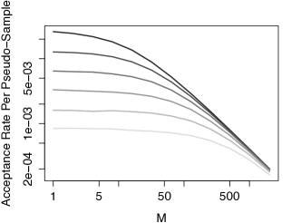
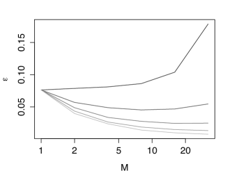
We now demonstrate these results through a simple simulation study, showing that choosing $M>1$ is seldom beneficial. We consider the model $\bm{y}|\bm{\theta}\sim\mathcal{N}(\bm{\theta},\sigma_{y}^{2})$ for a single observation $\bm{y}$, where $\sigma_{y}$ is known and $\bm{\theta}$ is given a standard normal prior, $\bm{\theta}\sim\mathcal{N}(0,1)$. We apply Algorithm 2 using proposal distribution $q(\bm{\theta}|\bm{\theta}^{(t-1)})=\mathcal{N}(\bm{\theta};0,1)$, summary statistic $\eta(\bm{y})=\bm{y}$, and $K(\eta)=\mathbf{1}_{\{\|\eta\|<\epsilon\}}$ equal to the uniform kernel with bandwidth $\epsilon$, and subsequently study the algorithm’s acceptance rate, which due to the independent proposal is analogous to effective sample size. We start by exploring the case where $\bm{y}_{\mathrm{obs}}=2$ and $\sigma_{y}=1$, simulating the Markov chain for $5$ million iterations. Figure 1 (left) shows the acceptance rate per generated pseudo-sample as a function of $M$. Large $M$ does not provide a benefit in terms of accepted $\bm{\theta}$ samples per generated pseudo-sample, and can even decrease this measure of efficiency, supporting the result of Corollary 5. In fact, replacing the uniform kernel with a Gaussian kernel (not shown) leads to indistinguishable results. In Figure 1 (right) we look at the $\epsilon$ which results from requiring that a fixed percentage ($0.4\%$) of $\bm{\theta}$ samples are accepted per unit computational cost. This means that for $M=1$ we require that $0.4\%$ of samples are accepted, while for $M=64$ we require that $0.4\times 64=25.6\%$ of samples are accepted.

In certain cases, there is an initial fixed computational cost to generating pseudo-samples, after which generating subsequent pseudo-samples is computationally inexpensive. If $\bm{y}$ is a length-$n$ sample from a Gaussian process, for instance, there is an initial $O(n^{3})$ cost to decomposing the covariance, after which each pseudo-sample may be generated at $O(n^{2})$ cost. In the case with discount factor $\delta>1$ (representing a $\delta\times$ cost reduction for all pseudo-samples after the first), the pseudo-sampling cost is $(1+(M-1)/\delta)$, so we require that $0.4\times(1+(M-1)/\delta)\%$ of $\bm{\theta}$ samples are accepted. For example, a discount of $\delta=16$ with $M=64$ requires that $2.0\%$ of samples are accepted. Figure 1 shows that, for $\delta=1$, larger $M$ results in larger $\epsilon$; in other words, for a fixed computational budget and no discount, $M=1$ gives the smallest $\epsilon$. For discounts $\delta>1$, however, increasing $M$ can indeed lead to reduced $\epsilon$.

Figure 1: Left: Acceptance rate per pseudo-sample. Lines correspond to $\epsilon=0.5^{2}$ (black) through $\epsilon=0.5^{6}$ (light grey), spaced uniformly on log scale. Right: The $\epsilon$ resulting from requiring that $0.4\%$ of $\bm{\theta}$ samples are accepted per unit computational cost. Lines correspond to different computational savings for pseudo-samples beyond the first, in the range $\delta=1$ (black, no cost savings), $2,4,8,16$ (light grey).

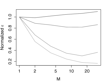
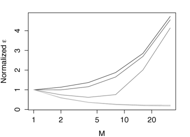
We further explore discounting in Figure 2, which uses a discount of $\delta=8$ and varies $\bm{y}_{\mathrm{obs}}$ from $2$ to $8$ (left plot) and $\sigma_{y}$ from $0.01$ to $2$ (right plot). In both cases the changes are meant to induce a divergence between the prior and the likelihood, and hence the prior and posterior. In these figures, the requisite $\epsilon$ are scaled such that at $M=1$ all normalized $\epsilon$ are $1$. Figure 2 (left) shows that as $\bm{y}_{\mathrm{obs}}$ grows, the benefit associated with using higher values of $M$ shrinks and eventually disappears. This is because for large $\bm{y}_{\mathrm{obs}}$ a large value of $\epsilon$ is required in order to frequently get a nonzero value for the approximated likelihood and thus a reasonable acceptance rate; for instance, the unnormalized value of $\epsilon$ is $0.08$ when $\bm{y}_{\mathrm{obs}}=2$ and $M=1$, while $\epsilon=7.64$ when $\bm{y}_{\mathrm{obs}}=8$ and $M=1$. As such, the increased diversity from multiple samples is dwarfed by the scale of $\epsilon$. In Figure 2 (right) we examine sensitivity of our conclusions to $\sigma_{y}$. For large $\sigma_{y}$, additional (discounted-cost) pseudo-samples provide a benefit, because they improve the accuracy of the approximated likelihood. However, for small values of $\sigma_{y}$, the variability of the pseudo-samples $y_{i,\bm{\theta}^{\prime}}$ is low and so additional pseudo-samples do not provide much incremental improvement to the likelihood approximation.

Figure 2: Sensitivity of the relationship between the bias and $M$ to changes in the likelihood. Each curve is normalized by dividing by its respective $\epsilon$ for $M=1$. Left: Varying $\bm{y}_{\mathrm{obs}}=2$ (light grey), $4,6,8$ (black). Right: Varying $\sigma_{y}=0.01$ (black), $0.05,0.1,0.5,1,2$ (light grey).

In summary, we only find a benefit of increasing the number of pseudo-samples $M$ in cases where there is a discounted cost to obtain those pseudo-samples, and even then the benefit can be decreased or eliminated when $\bm{y}_{\mathrm{obs}}$ is extreme under typical proposed values of $\bm{\theta}$, or when the variability of $\bm{y}$ under the model is low.

3 Discussion

In this paper, we have shown that despite the true likelihood leading to reduced asymptotic variance relative to the approximated likelihood constructed through ABC, in practice one should stick with simple, single pseudo-sample approximations rather than trying to accurately approximate the true likelihood with multiple pseudo-samples. Our results are obtained by bounding the asymptotic variance of Markov chain Monte Carlo estimates, which takes into account the autocorrelation of the Markov chain. This is not to say that $M=1$ is optimal in all situations. In many cases, there is a large initial cost to the first pseudo-sample, with subsequent samples drawn at a much reduced computational cost. In this case $M>1$ can lead to improved performance.

We hope that this work not only provides practical guidance on the choice of the number of pseudo-samples when using ABC, but also that it might lead to future research in the analysis of these algorithms. As a specific example, it would be fruitful to pursue the results in this paper extended to non-uniform kernels such as the popular Gaussian kernel. The main difficulty in doing so is extending the explicit calculation (A) in the proof of Proposition 4. Although we have found it possible to obtain similar bounds for specific kernels, target distributions and proposal distributions via grid search on a computer, and simulations suggest that our conclusions hold in greater generality, we have not been able to extend this inequality to general kernels and general target distributions simultaneously.

Appendix A Proofs

Proof of Theorem 3.

Denote by $H_{2,\alpha}$ the transition kernel of the pseudo-marginal algorithm with proposal kernel $q$, target marginal distribution $\mu$, and estimator $T_{2,x,\alpha}$ of the unnormalized target. If we denote by $\{(X_{t}^{(1)},T_{t}^{(1)})\}_{t\in\mathbb{N}}$ and $\{(X_{t}^{(2)},T_{t}^{(2)})\}_{t\in\mathbb{N}}$ the Markov chains driven by the kernels $H_{2,\alpha}$ and $\alpha\mathrm{I}+(1-\alpha)H_{2}$ respectively, then $\{X_{t}^{(1)}\}_{t\in\mathbb{N}}$ and $\{X_{t}^{(2)}\}_{t\in\mathbb{N}}$ have the same distribution.

If $T_{1,x}\leq_{cx}T_{2,x,\alpha}$ then by Theorem 3 of Andrieu2014establishing-some-order, v(f,H_1) &≤v(f, H_2,α) for any $f\in L^{2}(\mu)$. We also have

v(f, H_2,α) ≤11-α v(f,H_2) + α1 - α v(f) ≤1+ α1 - α v(f, H_2), where the first inequality follows from Corollary 1 of latuszynski2013clts and the second follows from the fact that $H_{2}$ has nonnegative spectrum. Combining this with (A) yields the desired result.

∎

Proof of Proposition 4.

For any $M\geq 1$, let $T_{M,\bm{\theta}}$ be the estimator $\hat{\pi}_{K,M}(\bm{\theta}|\bm{y}_{\mathrm{obs}})$ of the target $\pi_{K}$, so that $T_{M,\bm{\theta},\alpha}$ is $T_{M,\bm{\theta}}$ handicapped by $\alpha$ as defined in (2) of the main document. To obtain (4) of the main document, by Theorem 3 it is sufficient to take $\alpha=1-\frac{1}{M}$ and show that $T_{1,\bm{\theta}}\leq_{cx}T_{M,\bm{\theta},\alpha}$. By Proposition 2.2 of Lekela2014conditional-convex, it is furthermore sufficient to show that, for all $c\in\mathbb{R}$, E[—T_1,θ - c —] ≤E[—T_M,θ,α - c —].

Let $\mathrm{Bin}(n,\psi)$ denote the binomial distribution with $n$ trials and success probability $\psi$. For a given point $\bm{\theta}\in\Theta$, let $\tau=\tau(\bm{\theta})\equiv\mathbb{P}[T_{1,\bm{\theta}}\neq 0]=\int\textbf{1}_{\{\|\eta(\bm{y}_{\mathrm{obs}})-\eta(\bm{y})\|<\epsilon\}}p(\bm{y}|\bm{\theta})d\bm{y}$. Noting that $\frac{T_{1,\bm{\theta}}}{\pi(\bm{\theta})}\in\{0,1\}$, we may then write $T_{1,\bm{\theta}}$ and $T_{M,\bm{\theta},\alpha}$ as the following mixtures T1,θπ(θ) =D Bin(1,τ),   TM,θ,απ(θ) =D M-1M δ_0 + 1M Bin(M,τ), where $\delta_{0}$ is the unit point mass at zero. Denote $T_{1,\bm{\theta}}^{\prime}=\frac{T_{1,\bm{\theta}}}{\pi(\bm{\theta})}$ and $T_{M,\bm{\theta},\alpha}^{\prime}=\frac{T_{M,\bm{\theta},\alpha}}{\pi(\bm{\theta})}$. We will check condition (A) for $T_{1,\bm{\theta}}^{\prime},T_{M,\bm{\theta},\alpha}^{\prime}$ and $0\leq c\leq 1$, then separately for $c<0$ and $c>1$. For $0\leq c\leq 1$, we compute: E[—T_M,θ,α’ - c —] &= (1 - 1M ) c + 1M (1 - τ)^M c + 1M ( ∑_j=1^M M!j! (M-j)! τ^j (1-τ)^M-j ( j - c ) )
= τ+ c ( 1 - 2M( 1 - (1-τ)^M ) ) ≥τ+ c (1 - 2τ)  = E[—T_1,θ’ - c —]. For $c<0$, we have E[—T_M,θ,α’ - c —] = E[T_M,θ,α’] - c = E[T_1,θ’] - c = E[—T_1,θ’ - c —], and the analogous calculation gives the same conclusion for $c\geq M$. Finally, For $1<c<M$, note E[—T_1,θ’ - 1 —] ≤E[ —T_M,θ,α’ - 1 —],   E[—T_1,θ’ - M —] & = E[—T_M,θ,α’ - M —]. Also, the functions $f_{1}(c)\equiv\mathbb{E}[|T_{1,\bm{\theta}}^{\prime}-c|]$ and $f_{2}(c)\equiv\mathbb{E}[|T_{M,\bm{\theta},\alpha}^{\prime}-c|]$ are continuous, convex and piecewise linear. For $c\geq 1$, they satisfy ddc f_1(c) &= 1 ≥ddc f_2(c) where the derivative of $f_{2}$ exists. Combining inequalities (A) and (A), we conclude that E[—T_1,θ’ - c —] ≤E[—T_M,θ,α’ - c —] for all $1<c<M$. Thus we have verified (A) and the proposition follows. ∎

Appendix B Analysis of an Alternative ABC-MCMC Method

We give a result analogous to Corollary 2 for the version of ABC-MCMC proposed in wilk:08, given in Algorithm 3 below. The constant $c$ can be any value satisfying $c\geq\sup_{\bm{y}}K(\eta(\bm{y}_{\mathrm{obs}})-\eta(\bm{y}))$.

Initialize $\bm{\theta}^{(0)}$;

for $t=1$ to $n$ do

       Generate $\bm{\theta^{\prime}}\sim q(\cdot|\bm{\theta}^{(t-1)})$, $\bm{y}_{\bm{\theta}^{\prime}}\sim p(\bm{y}|\bm{\theta}^{\prime})$, and $u\sim\mbox{Uniform}[0,1]$;

       if $u\leq r(\bm{\theta}^{(t-1)},\bm{\theta}^{\prime}|\bm{y}_{\bm{\theta}^{\prime}})\equiv\frac{K(\eta(\bm{y}_{\mathrm{obs}})-\eta(\bm{y}_{\bm{\theta}^{\prime}}))}{c}\min\left\{1,\frac{\pi(\bm{\theta}^{\prime})q(\bm{\theta}^{(t-1)}|\bm{\theta}^{\prime})}{\pi(\bm{\theta}^{(t-1)})q(\bm{\theta}^{\prime}|\bm{\theta}^{(t-1)})}\right\}$, then

             Set $\bm{\theta}^{(t)}$ = $\bm{\theta^{\prime}}$

      else

             Set $\bm{\theta}^{(t)}$ = $\bm{\theta}^{(t-1)}$

Algorithm 3 Alternative ABC-MCMC Method

Lemma 6 compares Algorithm 3 (call its transition kernel $\tilde{Q}$) to $Q_{\infty}$.

Lemma 6.

For any $f\in L^{2}(\pi_{K})$ we have $v(f,\tilde{Q})\geq v(f,Q_{\infty})$.

Proof.

Both $\tilde{Q}$ and $Q_{\infty}$ have stationary density $\pi_{K}$, so by Theorem 4 of tierney1998ordering, it suffices to show that $Q_{\infty}(\bm{\theta},A\backslash\{\bm{\theta}\})\geq\tilde{Q}(\bm{\theta},A\backslash\{\bm{\theta}\})$ for all $\bm{\theta}\in\Theta$ and measurable $A\subset\Theta$. Since $\tilde{Q}$ and $Q_{\infty}$ use the same proposal density $q$, it is furthermore sufficient to show that for every $\bm{\theta}^{(t-1)}$ and $\bm{\theta}^{\prime}$, the acceptance probability of $Q_{\infty}$ is at least as large as that of $\tilde{Q}$. Since $p(\cdot|\bm{\theta})$ is a probability density,

$$\int K(\eta(\bm{y}_{\mathrm{obs}})-\eta(\bm{y}))p(\bm{y}|\bm{\theta})d\bm{y}\leq\sup_{\bm{y}}K(\eta(\bm{y}_{\mathrm{obs}})-\eta(\bm{y}))\qquad\forall\bm{\theta}\in\Theta.$$ (1)

So the acceptance probability of $\tilde{Q}$, marginalizing over $\bm{y}_{\bm{\theta}^{\prime}}$, is a_ABC &= ∫r(θ^(t-1), θ’ — y) p(y— θ’) d y
≤∫K(η(yobs)-η(y)) p(y— θ’) dysupyK(η(yobs)-η(y)) min{1,π(θ’) q(θ(t-1)—θ’)π(θ(t-1)) q(θ’ —θ(t-1))}
≤min{1, ∫K(η(yobs)-η(y)) p(y— θ’) dysupyK(η(yobs)-η(y)) (