Nodal bases for the serendipity family of finite elements

Abstract

Using the notion of multivariate lower set interpolation, we construct nodal basis functions for the serendipity family of finite elements, of any order and any dimension. For the purpose of computation, we also show how to express these functions as linear combinations of tensor-product polynomials.

1 Introduction

The serendipity family of $C^{0}$ finite elements is commonly used on cubical and parallelepiped meshes in two and three dimensions as a means to reduce the computational effort required by tensor-product elements. The number of basis functions of a tensor-product element of order $r$ in $n$ dimensions is $(r+1)^{n}$, while for a serendipity element it is asymptotically $\sim r^{n}/n!$ for large $r$, which represents a reduction of 50% in 2-D and 83% in 3-D. In this paper, we construct basis functions for serendipity elements of any order $r\geq 1$ in any number of dimensions $n\geq 1$, that are interpolatory at specified nodes and can be written as linear combinations of tensor-product polynomials (see equation (22)). The benefits and novelty of our approach are summarized as follows:

• Flexible node positioning. Our approach constructs nodal basis functions for any arrangement of points on the $n$-cube that respects the requisite association of degrees of freedom with sub-faces. In particular, we allow a symmetric arrangement of points that remains invariant under the symmetries of the $n$-cube.

• Tensor product decomposition. The basis functions we define are can be written as linear combinations of standard tensor product basis functions, with coefficients prescribed by a simple formula based on the geometry of a lower set of points associated to superlinear monomials.

• Dimensional nesting. The restriction of our basis functions for a $n$-cube to one of its $s$-dimensional faces coincides with the definition of our basis functions for an $s$-cube.

Serendipity elements have appeared in various mathematical and engineering texts, typically for small $n$ such as $n=2$ and $n=3$, and for small $r$; see BS2002 ; Ci02 ; G ; H1987 ; M1990 ; SB1991 ; SF73 ; LZ ; Z1998 . A common choice for the basis functions is a nodal (Lagrange) basis, which is an approach that has also been studied in the approximation theory literature. For example, Delvos D applied his ‘Boolean interpolation’ to construct a nodal basis for the case $n=3$ and $r=4$. Other bases have been considered, such as products of univariate Legendre polynomials, as in the work of Szabó and Babuška SB1991 .

It was relatively recently that the serendipity spaces were chacterized precisely for arbitrary $n$ and $r$, by Arnold and Awanou AA . They derived the polynomial space and its dimension, and also constructed a unisolvent set of degrees of freedom to determine an element uniquely. For the $n$-dimensional cube $I^{n}$, with $I=[-1,1]$, they defined the serendipity space $\mathcal{S}_{r}(I^{n})$ as the linear space of $n$-variate polynomials whose superlinear degree is at most $r$. The superlinear degree of a monomial is its total degree, less the number of variables appearing only linearly in the monomial. For a face $f$ of $I^{n}$ of dimension $d\geq 1$, the degrees of freedom proposed in AA for a scalar function $u$ are of the form

$$u\longmapsto\int_{f}uq,$$ (1)

for $q$ among some basis of $\mathcal{P}_{r-2d}(f)$. Here, $\mathcal{P}_{s}(f)$ is the space of restrictions to $f$ of $\mathcal{P}_{s}(I^{n})$, the space of $n$-variate polynomials of degree $\leq s$. These degrees of freedom were shown to be unisolvent by a hierarchical approach through the $n$ dimensions: the degrees of freedom at the vertices of $I^{n}$ are determined first (by evaluation); then the degrees of freedom on the 1-dimensional faces (edges), then those on the 2-dimensional faces, etc., finishing with those in the interior of $I^{n}$.

The approach of AA has the advantage that the degrees of freedom on any face $f$ of any dimension $d$ can be chosen independently of those on another face, of the same or of different dimension. Implementing a finite element method using these degrees of freedom, however, requires a set of ‘local basis functions’ that are associated to the integral degrees of freedom in some standardized fashion. The lack of simple nodal basis functions for this purpose has limited the broader use and awareness of serendipity elements.

The purpose of this paper is to show that by applying the notion of lower set interpolation in approximation theory and choosing an appropriate Cartesian grid in $I^{n}$, a nodal basis can indeed be constructed for the serendipity space $\mathcal{S}_{r}(I^{n})$ for any $n$ and $r$. The interpolation nodes are a subset of the points in the grid. The restrictions of the basis functions to any $d$-dimensional face are themselves basis functions of the same type for a $d$-cube, yielding $C^{0}$ continuity between adjacent elements.

If we keep all the nodes distinct, it is not possible to arrange them in a completely symmetric way for $r\geq 5$. However, lower set interpolation also applies to derivative data, and by collapsing interior grid coordinates to the midpoint of $I$, we obtain a Hermite-type basis of functions that are determined purely by symmetric interpolation conditions for all $n$ and $r$.

Lower set interpolation can also be expressed as a linear combination of tensor-product interpolants on rectangular subsets of the nodes involved DF . We derive an explicit formula for the coefficients in the serendipity case, which could be used for evaluation of the basis functions and their derivatives.

2 Interpolation on lower sets

A multi-index of $n$ non-negative integers will be denoted by

$$\alpha=(\alpha_{1},\alpha_{2},\ldots,\alpha_{n})\in\mathbb{N}_{0}^{n}.$$

For each $j=1,\ldots,n$, choose grid coordinates $x_{j,k}\in\mathbb{R}$ for all $k\in\mathbb{N}_{0}$, not necessarily distinct. These coordinates determine the grid points

$$x_{\alpha}:=(x_{1,\alpha_{1}},x_{2,\alpha_{2}},\ldots,x_{n,\alpha_{n}})\in\mathbb{R}^{n},\qquad\alpha\in\mathbb{N}_{0}^{n}.$$ (2)

The left multiplicity of $\alpha\in\mathbb{N}_{0}^{n}$ with respect to the $x_{j,k}$ is defined to be the multi-index

$$\rho(\alpha):=(\rho_{1}(\alpha),\ldots,\rho_{n}(\alpha))\in\mathbb{N}_{0}^{n},$$

where

$$\rho_{j}(\alpha):=\#\{k<\alpha_{j}:x_{j,k}=x_{j,\alpha_{j}}\}.$$ (3)

Thus $\rho_{j}(\alpha)$ is the number of coordinates in the sequence $x_{j,0},x_{j,1},\ldots,x_{j,\alpha_{j}-1}$ that are equal to $x_{j,\alpha_{j}}$. For each $\alpha\in\mathbb{N}_{0}^{n}$, we associate a linear functional $\lambda_{\alpha}$ as follows. Given any $u:\mathbb{R}^{n}\rightarrow\mathbb{R}$, defined with sufficiently many derivatives in a neighborhood of $x_{\alpha}$, let

$$\lambda_{\alpha}u:=D^{\rho(\alpha)}u(x_{\alpha}).$$

We call a finite set $L\subset\mathbb{N}_{0}^{n}$ a lower set if $\alpha\in L$ and $\mu\leq\alpha$ imply $\mu\in L$. The partial ordering $\mu\leq\alpha$ means $\mu_{j}\leq\alpha_{j}$ for all $j=1,\ldots,d$. We associate with $L$ the linear space of polynomials

$$P(L)={\rm span}\{x^{\alpha}:\alpha\in L\},$$ (4)

where

$$x^{\alpha}:=x_{1}^{\alpha_{1}}\cdots x_{n}^{\alpha_{n}},$$ (5)

for any point $x=(x_{1},\ldots,x_{n})\in\mathbb{R}^{n}$.

Polynomial interpolation on lower sets has been studied in CCS ; BR ; D ; DF ; GS2 ; Kuntzmann ; LL ; Muhlbach ; Sauer ; Werner and the following theorem has been established in various special cases by several authors.

Theorem 2.1

For any lower set $L\subset\mathbb{N}_{0}^{n}$ and a sufficiently smooth function $u:\mathbb{R}^{n}\rightarrow\mathbb{R}$, there is a unique polynomial $p\in P(L)$ that interpolates $u$ in the sense that

$$\lambda_{\alpha}p=\lambda_{\alpha}u,\qquad\alpha\in L.$$ (6)

The theorem leads to a basis of $P(L)$ with the basis function $\phi_{\alpha}\in P(L)$, $\alpha\in L$, defined by

$$\lambda_{\alpha^{\prime}}\phi_{\alpha}=\delta_{\alpha,\alpha^{\prime}},\qquad\alpha\in L,$$ (7)

where $\delta_{\alpha,\alpha^{\prime}}$ is 1 if $\alpha=\alpha^{\prime}$ and 0 otherwise. We can then express $p$ as

$$p(x)=\sum_{\alpha\in L}\phi_{\alpha}(x)\lambda_{\alpha}u.$$

3 Serendipity spaces

The serendipity space $\mathcal{S}_{r}(I^{n})$ can be described and partitioned using the language of lower sets. The standard norm for a multi-index $\alpha\in\mathbb{N}_{0}^{n}$ is

$$|\alpha|:=\sum_{j=1}^{n}\alpha_{j},$$

which is the degree of the monomial $x^{\alpha}$ in (5). We will define the superlinear norm of $\alpha$ to be

$$|\alpha|^{\prime}:=\sum_{\begin{subarray}{c}j=1\\ \alpha_{j}\geq 2\end{subarray}}^{n}\alpha_{j},$$

which is the ‘superlinear’ degree of $x^{\alpha}$ from AA . Using this we define, for any $r\geq 1$,

$$S_{r}:=\{\alpha\in\mathbb{N}_{0}^{n}:|\alpha|^{\prime}\leq r\}.$$ (8)

Observe that $S_{r}$ is a lower set since $|\alpha|^{\prime}\leq|\beta|^{\prime}$ whenever $\alpha\leq\beta$. Recalling (4), we let $\mathcal{S}_{r}=P(S_{r})$, which coincides with the definition of $\mathcal{S}_{r}$ in AA .

We now partition $S_{r}$, and hence $\mathcal{S}_{r}(I^{n})$, with respect to the faces of $I^{n}$. We can index these faces using a multi-index $\beta\in\{0,1,2\}^{n}$. For each such $\beta$ we define the face

$$f_{\beta}=I_{1,\beta_{1}}\times I_{2,\beta_{2}}\times\cdots\times I_{n,\beta_{n}},$$

where

$$I_{j,\beta_{j}}:=\begin{cases}-1,&\beta_{j}=0;\\ 1,&\beta_{j}=1;\\ (-1,1),&\beta_{j}=2.\end{cases}$$ (9)

Since $I$ can be written as the disjoint union $I=\{-1\}\cup\{1\}\cup(-1,1)$, we see that $I^{n}$ can be written as the disjoint union

$$I^{n}=\bigcup_{\beta\in\{0,1,2\}^{n}}f_{\beta}.$$

Hence, there are $3^{n}$ faces of all dimensions. The dimension of the face $f_{\beta}$ is

$$\dim f_{\beta}=\#\{j:\beta_{j}=2\},$$

and the number of faces of dimension $d$ is

$$\#\{f_{\beta}\subseteq I^{n}:\dim f_{\beta}=d\}=2^{n-d}\binom{n}{d}.$$ (10)

The $2^{n}$ vertices of $I^{n}$ correspond to $\beta\in\{0,1\}^{n}$, the $2^{n-1}n$ edges correspond to $\beta$ with exactly one entry equal to 2, and so forth, up to the single $n$-face, $f_{(2,2,\ldots,2)}$, the interior of $I^{n}$. To partition $S_{r}$ according to these faces, write $S_{r}$ as the disjoint union

$$S_{r}=\bigcup_{\beta\in\{0,1,2\}^{n}}S_{r,\beta},$$ (11)

where

$$S_{r,\beta}=\{\alpha\in S_{r}:\min(\alpha_{j},2)=\beta_{j},~{}\text{for}~{}j=1,\ldots,n\}.$$

We use this partition to compute the dimension of $S_{r}$ and confirm that it agrees with the dimension of $\mathcal{S}_{r}$ given in AA . Fix $\beta\in\{0,1,2\}^{n}$ and let $d=\dim f_{\beta}$. Letting $\mathbb{N}_{2}$ denote natural numbers $\geq 2$, we see that

$$\#S_{r,\beta}=\#\{\alpha\in\mathbb{N}_{2}^{d}:|\alpha|\leq r\}=\#\{\alpha\in\mathbb{N}_{0}^{d}:|\alpha|\leq r-2d\}.$$

Therefore,

$$\#S_{r,\beta}=\begin{cases}\binom{r-d}{d},&r\geq 2d;\\ 0,&\hbox{otherwise}.\end{cases}$$ (12)

Using (10), we thus find

$$\#S_{r}=\sum_{d=0}^{n}2^{n-d}\binom{n}{d}\#S_{r,\beta}=\sum_{d=0}^{\min(n,\lfloor r/2\rfloor)}2^{n-d}\binom{n}{d}\binom{r-d}{d},$$

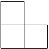
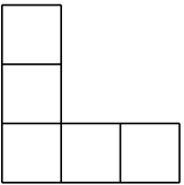
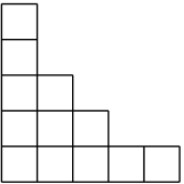
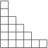
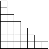
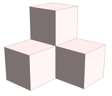
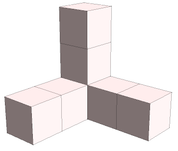
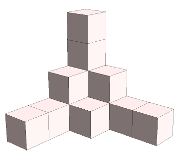
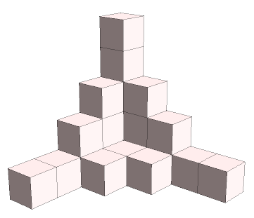
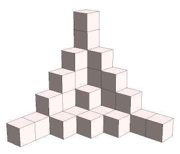
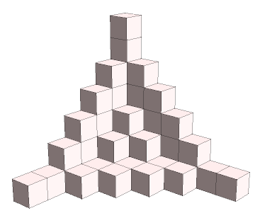
which is the formula for $\dim\mathcal{S}_{r}$ in (AA, , Equation (2.1)). A table of values of $\dim\mathcal{S}_{r}$ for small values of $n$ and $r$ is given in AA . Figures 1 and 2 show the set $S_{r}$ for $r=2,3,\ldots,7$ in 2-D and 3-D respectively.

Figure 1: For $n=2$, the geometry of the lower set $S_{r}$ is shown for $r=2,3,\ldots,7$. Treating each figure as a set of unit squares with the lower left corner at the origin in ${\mathbb{R}}^{2}$, the corners of each square indicate the points of ${\mathbb{N}}^{2}_{0}$ that belong to $S_{r}$.

Figure 2: For $n=3$, the geometry of the lower set $S_{r}$ is shown for $r=2,3,\ldots,7$. Treating each figure as a set of unit cubes based at the origin and viewed from first octant in ${\mathbb{R}}^{3}$, the corners of each cube indicate the points of ${\mathbb{N}}^{3}_{0}$ that belong to $S_{r}$.

4 Basis functions

We now apply Theorem 2.1 to the lower set $L=S_{r}$ to construct a nodal basis for $\mathcal{S}_{r}(I^{n})$ for arbitrary $r,n\geq 1$. To do this, we choose the grid coordinates $x_{j,k}$, $j=1,\ldots,n$, $k=0,\ldots,r$, in a manner that respects the indexing of the faces of $I^{n}$. Suppose that for $j=1,\ldots,n$,

$$x_{j,0}=-1\quad\hbox{and}\qquad x_{j,1}=1,$$

and

$$x_{j,k}\in(-1,1),\quad k=2,\ldots,r,$$

(not-necessarily distinct). Then for each $\beta\in\{0,1,2\}^{n}$, $x_{\alpha}\in f_{\beta}$ if and only if $\alpha\in S_{r,\beta}$.

Suppose further that the grid coordinates $x_{j,k}$, $k=2,\ldots,r$, are distinct. In this case the interpolation conditions of Theorem 2.1 are of Lagrange type:

$$p(x_{\alpha})=u(x_{\alpha}),\qquad\alpha\in S_{r},$$ (13)

giving the basis $\{\phi_{\alpha}:\alpha\in S_{r}\}$ for $\mathcal{S}_{r}(I^{n})$ defined by

$$\phi_{\alpha}(x_{\alpha^{\prime}})=\delta_{\alpha,\alpha^{\prime}},\qquad\alpha,\alpha^{\prime}\in S_{r}.$$

We consider two choices of such distinct coordinates. The first choice is to distribute them uniformly in $I$ in increasing order:

$$x_{j,k}=-1+\frac{2(k-1)}{r},\qquad k=2,\ldots,r,$$ (14)

as illustrated in Figure 3a. This configuration of nodes is, however, only symmetric for $r\leq 3$. Next, to obtain a more symmetric configuration, we re-order the interior grid coordinates in such a way that they are closer to the middle of $I$:

$$x_{j,r-2s} =1-\frac{2(s+1)}{r},\quad s=0,1,2,\ldots,\lfloor(r-2)/2\rfloor,$$ (15)

$$x_{j,r-2s-1} =-1+\frac{2(s+1)}{r},\quad s=0,1,2,\ldots,\lfloor(r-3)/2\rfloor.$$ (16)

as illustrated in Figure 3b. This yields a symmetric configuration for $r\leq 4$, but not for $r\geq 5$. This lack of symmetry motivates the third choice of letting all interior grid coordinates coalesce to the midpoint of $I$, i.e.,

$$x_{j,k}=0,\qquad k=2,\ldots,r,$$ (17)

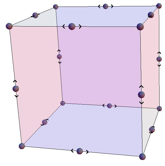
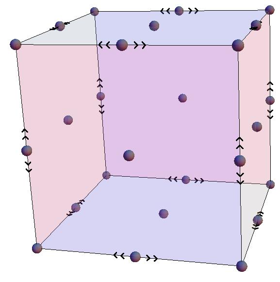
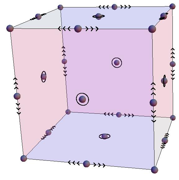
as indicated in Figure 3c. This gives interpolation conditions that are symmetric for all $n$ and $r$, but the trade-off is that these conditions are now of Hermite type rather than Lagrange.

$(a)$	$(b)$	$(c)$

Figure 3: Three choices of $x_{j,k}$, $2\leq k\leq 5$, for $n=2$, $r=5$. The first two choices are Lagrange-like while the third is Hermite-like.

In this Hermite case, all the points $x_{\alpha}$ in the face $f_{\beta}$ are equal to the mipoint of that face, which we denote by $y_{\beta}$. The interpolation conditions of Theorem 2.1 then become

$$D^{\rho}p(y_{\beta})=D^{\rho}u(y_{\beta}),\qquad\beta\in\{0,1,2\}^{n},\quad\rho\in K_{r,\beta},$$ (18)

where

$$K_{r,\beta}:=\{\rho\in\mathbb{N}_{0}^{n}:|\rho|\leq r-2d~{}\text{with}~{}\rho_{j}=0~{}\text{if}~{}\beta_{j}<2\}.$$ (19)

Thus $p$ can be expressed as

$$p(x)=\sum_{\beta\in\{0,1,2\}^{n}}\sum_{\rho\in K_{r,\beta}}D^{\rho}u(y_{\beta})\phi_{\beta,\rho}(x),$$

where

$$\{\phi_{\beta,\rho}:\beta\in\{0,1,2\}^{n},\rho\in K_{r,\beta}\}$$

is a basis for $\mathcal{S}_{r}$ defined by

$$D^{\rho^{\prime}}\phi_{\beta,\rho}(y_{\beta^{\prime}})=\delta_{\beta,\beta^{\prime}}\delta_{\rho,\rho^{\prime}},\;\;\text{for any}\;\;\beta^{\prime}\in\{0,1,2\}^{n},\;\rho^{\prime}\in K_{r,\beta}.$$

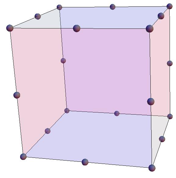
Figure 4 illustrates these interpolation conditions for $r=2$ through $r=5$ in the case $n=3$.

Figure 4: Hermite-like interpolation conditions in 3-D for $r=2,3,4,5$. A dot indicates that a basis function will interpolate the value of the function at that location. A dot on an edge enclosed by $\ell$ sets of parentheses indicates that basis functions will interpolate each partial derivative along the edge at the location of the dot, up to order $\ell$. A dot in the interior enclosed by $\ell$ circles indicates that basis functions will interpolate all partial derivatives at the location of dot, up to total order $\ell$.

5 Tensor-product formula

In this last section we explain how the interpolant can be expressed as a linear combination of tensor-product interpolants over various rectangular subgrids of the overall grid. This applies also to the basis functions and so gives a simple method of evaluating these functions and their derivatives. To do this we apply the formula recently obtained in DF . Suppose again that $L\subset\mathbb{N}_{0}^{n}$ is any lower set as in Section 2 and consider the interpolant $p$ to $u$ in Theorem 2.1. For any $\alpha\in L$ define the rectangular block

$$B_{\alpha}=\{\mu\in\mathbb{N}_{0}^{n}:\mu\leq\alpha\}$$

and let $p_{\alpha}\in P(B_{\alpha})$ denote the tensor-product interpolant to $u$ satisfying the interpolation conditions (6) for $\mu\in B_{\alpha}$. Further, let $\chi(L):\mathbb{N}_{0}^{n}\to\{0,1\}$ be the characteristic function defined by

$$\chi(L)(\alpha)=\begin{cases}1&\hbox{if $\alpha\in L$;}\\ 0&\hbox{otherwise.}\\ \end{cases}$$

It was shown in DF that

$$p=\sum_{\alpha\in L}c_{\alpha}p_{\alpha},$$ (20)

where

$$c_{\alpha}=\sum_{\epsilon\in\{0,1\}^{n}}(-1)^{|\epsilon|}\chi(L)(\alpha+\epsilon),\qquad\alpha\in L.$$ (21)

This in turn gives a formula for each basis function $\phi_{\beta}\in P(L)$, i.e.,

$$\phi_{\beta}(x)=\sum_{\begin{subarray}{c}\alpha\in L\\ \alpha\geq\beta\end{subarray}}c_{\alpha}\phi_{\beta,\alpha},$$ (22)

where $\phi_{\beta,\alpha}\in P(B_{\alpha})$ denotes the tensor-product basis function associated with the index $\beta$, defined by

$$\lambda_{\beta^{\prime}}\phi_{\beta,\alpha}=\delta_{\beta,\beta^{\prime}},\qquad\beta\in B_{\alpha}.$$

For a general lower set $L$, many of the integer coefficients $c_{\alpha}$ are zero, and so in order to apply (20) to evaluate $p$ we need to determine which of the $c_{\alpha}$ are non-zero, and to find their values. With $L=S_{r}$ we could do this in practice by implementing the formula (21). However, we will derive a specific formula for the $c_{\alpha}$. We call $\alpha\in L$ a boundary point of $L$ if $\alpha+1_{n}\not\in L$, where $1_{n}=(1,1,\ldots,1)\in\mathbb{N}_{0}^{n}$. Let $\partial L$ denote the set of boundary points of $L$. As observed in DF , if $\alpha$ is not a boundary point then $c_{\alpha}=0$.

Consider now the formula (20) when $L=S_{r}$. Note that $|\alpha|^{\prime}$ is a symmetric function of $\alpha$: it is unchanged if we swap $\alpha_{j}$ and $\alpha_{i}$ for $i\neq j$. It follows that $\chi(S_{r})(\alpha)$ is also symmetric in $\alpha$, and therefore $c_{\alpha}$ is also symmetric in $\alpha$. We can thus determine the boundary points $\alpha\in\partial S_{r}$ and their coefficients $c_{\alpha}$ according to how many zeros and ones $\alpha$ contains. For any $\alpha\in\mathbb{N}_{0}^{n}$ let $m_{i}(\alpha)$ denote the multiplicity of the integer $i\geq 0$ in $(\alpha_{1},\ldots,\alpha_{n})$, i.e.,

$$m_{i}(\alpha)=\#\{\alpha_{j}=i\}.$$

Lemma 1

If $\alpha\in\partial S_{r}$ and $m_{0}(\alpha)\geq 1$ then $c_{\alpha}=0$.

Proof

By the symmetry of $c_{\alpha}$ we may assume that $\alpha_{1}=0$, and from (21) we can express $c_{\alpha}$ as

$$c_{\alpha}=\sum_{\epsilon\in\{0\}\times\{0,1\}^{n-1}}(-1)^{|\epsilon|}\big{(}\chi(S_{r})(\alpha+\epsilon)-\chi(S_{r})(\alpha+e_{1}+\epsilon)\big{)},$$

where $e_{1}=(1,0,\ldots,0)\in\mathbb{N}_{0}^{n}$. Since $\alpha_{1}=0$, both

$$(\alpha+\epsilon)_{1}\leq 1\qquad\hbox{and}\qquad(\alpha+e_{1}+\epsilon)_{1}\leq 1,$$

and so

$$|\alpha+\epsilon|^{\prime}=|\alpha+e_{1}+\epsilon|^{\prime},$$

and therefore

$$\chi(S_{r})(\alpha+\epsilon)=\chi(S_{r})(\alpha+e_{1}+\epsilon),$$

and so $c_{\alpha}=0$.

In view of Lemma 1, we need only consider points $\alpha\in\partial S_{r}\cap\mathbb{N}_{1}^{n}$.

Lemma 2

Let $\alpha\in S_{r}\cap\mathbb{N}_{1}^{n}$ and $m_{1}=m_{1}(\alpha)$. Then $\alpha\in\partial S_{r}$ if and only if

$$|\alpha|^{\prime}>r-(n+m_{1}).$$

Proof

By the definition of $S_{r}$, $\alpha\in\partial S_{r}$ if and only if $|\alpha+1_{n}|^{\prime}>r$. Since $\alpha\in\mathbb{N}_{1}^{n}$,

$$\#\{\alpha_{j}\geq 2\}=n-m_{1},$$

and we find

$$|\alpha+1_{n}|^{\prime}=2m_{1}+|\alpha|^{\prime}+(n-m_{1})=|\alpha|^{\prime}+n+m_{1},$$

which proves the result.

In view of Lemma 2, we need only consider points $\alpha\in\mathbb{N}_{1}^{n}$ such that

$$|\alpha|^{\prime}=r-k,\qquad k=0,1,\ldots,n+m-1,$$ (23)

where $m=m_{1}(\alpha)$.

Theorem 5.1

Let $\alpha\in\mathbb{N}_{1}^{n}$ be as in (23). If $m<n$ then

$$c_{\alpha}=c_{m,k}:=\sum_{i=0}^{m}(-1)^{k+i}\binom{m}{i}\binom{n-m-1}{k-2i},$$ (24)

with the convention that $\binom{l}{j}=0$ if $j<0$ or $j>l$.

Proof

Let $\epsilon\in\{0,1\}^{n}$, and let

$$i_{1}=\#\{j:\hbox{$\epsilon_{j}=1$ and $\alpha_{j}=1$}\},$$

$$i_{2}=\#\{j:\hbox{$\epsilon_{j}=1$ and $\alpha_{j}\geq 2$}\}.$$

Then

$$|\alpha+\epsilon|^{\prime}=|\alpha|^{\prime}+2i_{1}+i_{2},$$

and so $\alpha+\epsilon\in S_{r}$ if and only if

$$|\alpha|^{\prime}+2i_{1}+i_{2}\leq r,$$

or, equivalently,

$$2i_{1}+i_{2}\leq k.$$

Since the number of ways of choosing $i_{1}$ elements among $m$ is $\binom{m}{i_{1}}$, and the number of ways of choosing $i_{2}$ elements among $n-m$ is $\binom{n-m}{i_{2}}$ the sum in (21) reduces to

$$c_{\alpha}=\sum_{i_{1}=0}^{m}\sum_{i_{2}=0}^{k-2i_{1}}(-1)^{i_{1}+i_{2}}\binom{m}{i_{1}}\binom{n-m}{i_{2}}.$$

Since

$$\sum_{i_{2}=0}^{k-2i_{1}}(-1)^{i_{2}}\binom{n-m}{i_{2}}=(-1)^{k-2i_{1}}\binom{n-m-1}{k-2i_{1}},$$

we obtain (24).

Table 1 shows the values of the coefficients $c_{m,k}$ for $n=1,2,3,4$.

					$k$
$n$	$m$	$0$	$1$	$2$	$3$	$4$	$5$	$6$
$1$	0	1
$2$	0	1	-1
	1	1	0	-1
$3$	0	1	-2	1
	1	1	-1	-1	1
	2	1	0	-2	0	1
$4$	0	1	-3	3	-1
	1	1	-2	0	2	-1
	2	1	-1	-2	2	1	-1
	3	1	0	-3	0	3	0	-1

Table 1: Coefficients $c_{m,k}$ for $n=1,2,3,4$.

Finally, we need to consider the possibility that $m=n$ in (23), in which case the formula (24) is no longer valid, and we must treat this situation separately. In this case $\alpha=1_{n}$ and we can again find $c_{\alpha}$ from (21). Since

$$|1_{n}+1_{n}|^{\prime}=|2_{n}|^{\prime}=2n,$$

we see that $1_{n}\in\partial S_{r}$ if and only if $r<2n$.

Theorem 5.2

Suppose that $r<2n$. Then

$$c_{1_{n}}=(-1)^{\lfloor r/2\rfloor}\binom{n-1}{\lfloor r/2\rfloor}.$$ (25)

Proof

For any $\epsilon\in\{0,1\}^{n}$,

$$|1_{n}+\epsilon|^{\prime}=2|\epsilon|,$$

and so (21) gives

$$c_{1_{n}}=\sum_{\begin{subarray}{c}\epsilon\in\{0,1\}^{n}\\ 2|\epsilon|\leq r\end{subarray}}(-1)^{|\epsilon|}=\sum_{i=0}^{\lfloor r/2\rfloor}\binom{n}{i}(-1)^{i}$$

which gives (25).

We now consider examples of the use of Theorems 5.1 and 5.2, and let $p_{r}$ denote the interpolant $p$ in Theorem 2.1 when $L=S_{r}$.

5.1 2-D case

For $n=2$, Theorems 5.1 and 5.2 give

$$p_{1} =p_{11},$$

$$p_{2} =p_{21}+p_{12}-p_{11},$$

$$p_{3} =p_{31}+p_{13}-p_{11},$$

$$p_{4} =p_{41}+p_{14}+p_{22}-(p_{21}+p_{12}),$$

$$p_{5} =p_{51}+p_{15}+p_{32}+p_{23}-(p_{31}+p_{31}+p_{22}).$$

Figure 5 shows the polynomials in $S_{5}$ in the formula for $p_{5}$, with black if $c_{\alpha}=1$ and white if $c_{\alpha}=-1$.

Figure 5: The geometry of $S_{5}$ for $n=2$ is shown (see Figure 1) with an indication of which blocks within the set contribute to the representation of the serendipity interpolant $p_{5}$ as a linear combination of tensor product interpolants. A block with a filled dot in the upper right corner contributes with coefficient +1 while a block with an empty dot in the upper right corner contributes with coefficient $-1$.

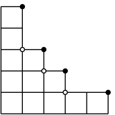
Figure 6 depicts the polynomials in the same formula, based on the Hermite interpolation conditions (17).

		$+$		$+$		$+$
$-$		$-$		$-$		$=$

Figure 6: A visual depiction of the the formula for $p_{5}$ in the Hermite case.

5.2 3-D case

For $n=3$, to simplify the formulas let

$$q_{\alpha}:=\sum_{\alpha^{\prime}\in\pi(\alpha)}p_{\alpha^{\prime}},$$

with $\pi(\alpha)$ denoting all permutations of $\alpha=(\alpha_{1},\alpha_{2},\alpha_{3})$, so that, for example,

$$q_{111} :=p_{111},$$

$$q_{112} :=p_{112}+p_{121}+p_{211},$$

$$q_{123} :=p_{123}+p_{132}+p_{213}+p_{231}+p_{312}+p_{323},$$

etc. Then Theorems 5.1 and 5.2 give

$$p_{1} =q_{111},$$

$$p_{2} =q_{112}-2q_{111},$$

$$p_{3} =q_{113}-2q_{111},$$

$$p_{4} =q_{122}+(q_{114}-2q_{112})+q_{111},$$

$$p_{5} =(q_{123}-q_{122})+(q_{115}-2q_{113})+q_{111}.$$

We note that Delvos D found a nodal basis for $p_{4}$, $n=3$, using his method of ‘Boolean interpolation.’ That method is not, however, general enough to give the formulas for $p_{r}$ with $r\geq 5$, $n=3$. Now that we have provided a generalized approach to defining nodal bases for serendipity elements, it remains to be studied whether certain arrangements of the grid coordinates $x_{j,k}$ provide advantages in specific application contexts. Suitable pre-conditioners associated to these bases may also be needed.

References

- (1) Arnold, D., Awanou, G.: The serendipity family of finite elements. Foundations of Computational Mathematics 11(3), 337–344 (2011)
- (2) Brenner, S., Scott, L.: The Mathematical Theory of Finite Element Mehtods. Springer-Verlag, New York (2002)
- (3) Chkifa, A., Cohen, A., Schwab, C.: High-dimensional adaptive sparse polynomial interpolation and applications to parametric pdes. Foundations of Computational Mathematics pp. 1–33 (2012)
- (4) Ciarlet, P.: The Finite Element Method for Elliptic Problems, Classics in Applied Mathematics, vol. 40, second edn. SIAM, Philadelphia, PA (2002)
- (5) De Boor, C., Ron, A.: On multivariate polynomial interpolation. Constructive Approximation 6(3), 287–302 (1990)
- (6) Delvos, F.J.: -variate boolean interpolation. Journal of Approximation Theory 34(2), 99–114 (1982)
- (7) Dyn, N., Floater, M.: Multivariate polynomial interpolation on lower sets. Journal of Approximation Theory 177(1), 34–42 (2014)
- (8) Gasca, M., Sauer, T.: Polynomial interpolation in several variables. Advances in Computational Mathematics 12(4), 377–410 (2000)
- (9) Gillette, A.: Hermite and Bernstein style basis functions for cubic serendipity spaces on squares and cubes. In: Approximation Theory XIV: San Antonio 2013, pp. 103–121. Springer (2014)
- (10) Hughes, T.J.R.: The finite element method. Prentice Hall Inc., Englewood Cliffs, NJ (1987)
- (11) Kuntzmann, J.: Méthodes numériques: interpolation, dérivées. Dunod Paris (1959)
- (12) Lin, R., Zhang, Z.: Natural superconvergence points in three-dimensional finite elements. SIAM Journal on Numerical Analysis 46(3), 1281–1297 (2008)
- (13) Lorentz, G.G., Lorentz, R.A.: Solvability problems of bivariate interpolation I. Constructive approximation 2(1), 153–169 (1986)
- (14) Mandel, J.: Iterative solvers by substructuring for the -version finite element method. Computer Methods in Applied Mechanics and Engineering 80(1-3), 117–128 (1990)
- (15) Mühlbach, G.: On multivariate interpolation by generalized polynomials on subsets of grids. Computing 40(3), 201–215 (1988)
- (16) Sauer, T.: Lagrange interpolation on subgrids of tensor product grids. Mathematics of Computation 73(245), 181–190 (2004)
- (17) Strang, G., Fix, G.J.: An analysis of the finite element method. Prentice-Hall Inc., Englewood Cliffs, N. J. (1973)
- (18) Szabó, B., Babuška, I.: Finite element analysis. Wiley-Interscience (1991)
- (19) Werner, H.: Remarks on newton type multivariate interpolation for subsets of grids. Computing 25(2), 181–191 (1980)
- (20) Zhang, Z.: Derivative superconvergent points in finite element solutions of Poisson’s equation for the serendipity and intermediate families-a theoretical justification. Mathematics of Computation of the American Mathematical Society 67(222), 541–552 (1998)