Scalable Similarity Learning using Large Margin Neighborhood Embedding

Abstract

Classifying large-scale image data into object categories is an important problem that has received increasing research attention. Given the huge amount of data, non-parametric approaches such as nearest neighbor classifiers have shown promising results, especially when they are underpinned by a learned distance or similarity measurement. Although metric learning has been well studied in the past decades, most existing algorithms are impractical to handle large-scale data sets. In this paper, we present an image similarity learning method that can scale well in both the number of images and the dimensionality of image descriptors. To this end, similarity comparison is restricted to each sample’s local neighbors and a discriminative similarity measure is induced from large margin neighborhood embedding. We also exploit the ensemble of projections so that high-dimensional features can be processed in a set of lower-dimensional subspaces in parallel without much performance compromise. The similarity function is learned online using a stochastic gradient descent algorithm in which the triplet sampling strategy is customized for quick convergence of classification performance. The effectiveness of our proposed model is validated on several data sets with scales varying from tens of thousands to one million images. Recognition accuracies competitive with the state-of-the-art performance are achieved with much higher efficiency and scalability.

1 Introduction

As the number of digital images generated and uploaded to the Internet skyrockets, automatic categorization of large-scale image sets with diversified contents has become a popular research topic [1, 2, 3]. The conventional approach to train a classifier for each class using one-versus-all paradigm is usually unscalable to such a large number of images and classes, not to mention that the sizes of most web data are constantly growing. On the other hand, as the vast amount of image samples populate the data space more densely, we can now afford classification models with higher capacities to capture the underlying data distribution. Non-parametric methods, which infer the label information of test images from similar database images, have demonstrated promising results on large data sets in many vision tasks including scene parsing [4], object detection [5], face alignment [6], etc. For classification, the non-parametric k-Nearest Neighbor (kNN) classifier [7] has been successfully applied on the ImageNet Challenge data set [8].

A good distance or similarity measure is crucial to the performance of any non-parametric model. As most image feature descriptors have very high dimensions and mainly characterize the low level visual information, measuring their distance directly in the Euclidian space yields unsatisfactory results. In order to close the semantic gap, people have used supervised information [9] to learn distance metrics with promoted semantic similarity, famous examples include information-theoretic [10] and large margin nearest neighbor (LMNN) [11] methods. The supervision is usually provided in the form of comparative constraints over image pairs, triplets or even quadruplets [12], leading to a time complexity which grows polynomially with sample size. In addition, for large-scale data where multi-modal distributions are usually observed, a single distance metric is insufficient to correctly measure the similarities between all image pairs throughout the space. To ameliorate the problem, multiple metrics have been applied to different parts of the data space, by either assigning a distinct metric to each discrete space partition [13, 14] or learning an adaptive metric parameterized based on the location of test sample [15, 16, 17, 18, 19]. However, the extra model complexity of local metrics makes them less suitable for large-scale applications.

Besides the size of data sets, the high dimensionality of image descriptors is another factor limiting the scalability of existing metric learning algorithms. The Mahalanobis distance, one of the most popular forms of distance metric, requires computation quadratic to data dimension in calculation and cubic to dimension in its learning when positive-semidefinite constraint is placed. Low-rank regularization can be imposed on the Mahalanobis metric to save computation, but this may result in a non-convex optimization problem [20] and cause performance loss in some cases. Kernel function is useful in reducing the number of free metric parameters [21], but it does not scale up well to the number of samples.

In this paper, we propose a new similarity learning algorithm that features good scalability with respect to both sample size and dimensionality. First, motivated by the findings from manifold learning with neighborhood embedding [22, 23], we restrict similarity comparison to sample pairs within the same local neighborhood, and try to capture the discriminative structure of local data manifold using large margin neighborhood embedding (Sec. 2). In this way, we can not only save a great amount of computation in training and testing, but also gain robustness to outliers by focusing only on more relevant samples, which shares the same rationale as the method in [24]. On the other hand, we project the original high-dimensional data to a set of lower-dimensional subspaces, and use the ensemble of similarities learned from these subspaces as a surrogate to the similarity in original space (Sec. 3). The similarity for each subspace can be evaluated and optimized in parallel, which offers superior scalability to data dimension. The proposed method is validated on several image classification benchmarks with varying scales (Sec. 4), and both of its accuracy and efficiency are shown to scale up gracefully from tens of thousands to one million images. Potential extensions of this work are also discussed (Sec. 5). In short, the main contributions of this paper are:

• a neighborhood embedding based similarity learning algorithm with improved classification performance and better scalability to the number of training samples;

• an ensemble of distributed similarities learning algorithm which scales well to data dimensionality.

2 Similarity Learning using Neighborhood Embedding

Graph embedding [22] is a family of dimensionality reduction algorithms which map data points from a manifold in high-dimensional space to low-dimensional space while preserving the intrinsic data structure represented by a weighted graph. In many cases such as Locally Linear Embedding (LLE) [25] and Laplacian eigenmap [26], a sparsely-connected graph is constructed based on neighborhood relationship, which we refer to as neighborhood embedding.

Since learning the transform of dimensionality reduction can be regarded as a special case of distance or similarity learning, it is easy to extend the concept of neighborhood embedding to similarity learning. Given a set of $N$ data samples $\{\mathbf{x}_{i}\}_{i=1}^{N}$ and the associated class labels $\{y_{i}\}_{i=1}^{N}$, we define $\mathcal{N}_{i}$ as the index set for $\mathbf{x}_{i}$’s $k$ nearest neighbors (in Euclidean distance). $\mathcal{N}_{i}$ can be divided into two mutually exclusive subsets $\mathcal{N}^{+}_{i}$ and $\mathcal{N}^{-}_{i}$, which denote the indices of $\mathbf{x}_{i}$’s neighbors with and not with label $y_{i}$, respectively. An adjacency graph can be built in which each $\mathbf{x}_{i}$ is a vertex, and there is an undirected edge with weight $w_{ij}$ linking $\mathbf{x}_{i}$ and $\mathbf{x}_{j}$ if $i\in\mathcal{N}_{j}$ or $j\in\mathcal{N}_{i}$. Generally, neighborhood embedding tries to find an optimal transform $f$ for all the data samples by minimizing the following loss function:

$$\mathcal{L}=\sum_{i\in\mathcal{N}_{j}\vee j\in\mathcal{N}_{i}}w_{ij}d\left(f(\mathbf{x}_{i}),f(\mathbf{x}_{j})\right),$$ (1)

where $f$ is usually a linear transform and $d(\cdot,\cdot)$ is the Euclidean distance measure in the transformed space. For our purpose, we are interested in a good similarity function $s(\mathbf{x}_{i},\mathbf{x}_{j})$ defined as a mapping from a pair of samples $(\mathbf{x}_{i},\mathbf{x}_{j})$ to a real number that quantifies their semantic similarity. Here we adopt a bilinear similarity function parameterized by a matrix $\mathbf{M}$:

$$s_{\mathbf{M}}(\mathbf{x}_{i},\mathbf{x}_{j})=\mathbf{x}_{i}^{T}\mathbf{M}\mathbf{x}_{j},$$ (2)

and $\mathbf{M}$ is a symmetric matrix usually with a low rank constraint. Bilinear similarity is commonly used in place of distance metric for its compactness [27, 28]. Its performance in many recognition tasks is found to be similar as the Mahalanobis distance, which has better theoretical properties but requires a positive semidefinite parameter matrix. With the neighborhood embedding formulation, the objective for similarity learning can be cast as

$$\min_{\mathbf{M}}\mathcal{L}(\mathbf{M})=\sum_{i\in\mathcal{N}_{j}\vee j\in\mathcal{N}_{i}}w_{ij}s_{\mathbf{M}}(\mathbf{x}_{i},\mathbf{x}_{j}).$$ (3)

We still need to define the weights $w_{ij}$, which encode the class label information. Binary values ${\pm}1$ are commonly used to assign $w_{ij}$ based on whether $\mathbf{x}_{i}$ and $\mathbf{x}_{j}$ come from the same class or not [23], which essentially has the same effect as partitioning the adjacency graph into a within-class graph and a between-class graph [22, 29, 30] to impose a pairwise constraint that the similarity should be high between samples from the same class and low otherwise. For kNN classifiers, as suggested in [11], we care more about the relative similarity defined over a triplet of samples; i.e., a higher similarity score should be assigned when a sample $\mathbf{x}_{i}$ is compared with any of its target neighbor $\mathbf{x}_{j},j{\in}\mathcal{N}^{+}_{i}\vee i{\in}\mathcal{N}^{+}_{j}$ than with any of its imposter neighbor $\mathbf{x}_{l},l{\in}\mathcal{N}^{-}_{i}\vee i{\in}\mathcal{N}^{-}_{l}$. To this end, we define the graph weights as

$$w_{ij}=\left\{\begin{array}[]{rl}-|\{l|l{\in}\mathcal{N}^{-}_{i}\vee i{\in}\mathcal{N}^{-}_{l}\}|,&j{\in}\mathcal{N}^{+}_{i}\vee i{\in}\mathcal{N}^{+}_{j}\\ +|\{l|l{\in}\mathcal{N}^{+}_{i}\vee i{\in}\mathcal{N}^{+}_{l}\}|,&j{\in}\mathcal{N}^{-}_{i}\vee i{\in}\mathcal{N}^{-}_{j}\\ 0,&\mathrm{otherwise}\end{array}\right.,$$ (4)

where $|\mathcal{A}|$ denotes the cardinality of set $\mathcal{A}$. With the weights in (4), we can organize our objective function into a more interpretable form:

$$\mathcal{L}(\mathbf{M})=\sum_{i}\sum_{j\in\mathcal{N}^{+}_{i}\vee i\in\mathcal{N}^{+}_{j}}\sum_{l\in\mathcal{N}^{-}_{i}\vee i\in\mathcal{N}^{-}_{l}}-s_{\mathbf{M}}(\mathbf{x}_{i},\mathbf{x}_{j})+s_{\mathbf{M}}(\mathbf{x}_{i},\mathbf{x}_{l}),$$ (5)

which enforces relative similarity constraint for each triplet $(\mathbf{x}_{i},\mathbf{x}_{j},\mathbf{x}_{l})$ from the same neighborhood. To apply more penalty to those triplets violating the constraint, we use a hinge function to promote large margin of relative similarity difference, leading to the final form of our objective:

$$\min_{\mathbf{M}}\mathcal{L}(\mathbf{M})=\sum_{i}\sum_{j\in\mathcal{N}^{+}_{i}\vee i\in\mathcal{N}^{+}_{j}}\sum_{l\in\mathcal{N}^{-}_{i}\vee i\in\mathcal{N}^{-}_{l}}\left[b-s_{\mathbf{M}}(\mathbf{x}_{i},\mathbf{x}_{j})+s_{\mathbf{M}}(\mathbf{x}_{i},\mathbf{x}_{l})\right]_{+},$$ (6)

where $[\cdot]_{+}=\max(\cdot,0)$ is the hinge loss function, and $b>0$ is the minimum required margin by which $\mathbf{x}_{i}$ should be more similar to a target neighbor $\mathbf{x}_{j}$ than to an imposter neighbor $\mathbf{x}_{l}$ as measured by $s_{\mathbf{M}}(\cdot,\cdot)$.

2.1 Learning Algorithm

Optimal linear transforms for neighborhood embedding can be found by solving a generalized eigen decomposition problem using graph Laplacian. However, this approach is not applicable for large-scale data and the nonlinear objective in Eq. (6). Instead, we use an online learning method based on stochastic gradient descent [31], which is similar to [7, 27]. Specifically, we iteratively go through the whole training set and randomly sample triplet $\{\mathbf{x}_{i},\mathbf{x}_{j},\mathbf{x}_{l}\}$ which contributes non-zero cost to the objective in (6). The sub-gradient of the objective evaluated at the current triplet is then used to update the parameter $\mathbf{M}$. The update is performed iteratively with a diminishing step size and terminates upon convergence.

There can be a huge number of triplets to be considered in the objective function (6), even though the similarity comparison is restricted to local neighbors. Thus, a good sampling strategy to generate candidate triplets is essential to the speed of convergence on large data sets. For each training sample $\mathbf{x}_{i}$, we search for its target neighbor $\mathbf{x}_{j}$ and imposter neighbor $\mathbf{x}_{l}$ according to

$$\{j,l\}= \arg\max_{j^{\prime},l^{\prime}}s_{\mathbf{M}}(\mathbf{x}_{i},\mathbf{x}_{l^{\prime}})-s_{\mathbf{M}}(\mathbf{x}_{i},\mathbf{x}_{j^{\prime}}),$$

$$\mathrm{s.t.}\;\;\;\;j^{\prime}\in\mathcal{N}^{+}_{i}\vee i\in\mathcal{N}^{+}_{j^{\prime}},\;\;l^{\prime}\in\mathcal{N}^{-}_{i}\vee i\in\mathcal{N}^{-}_{l^{\prime}}.$$ (7)

Optimizing (2.1) returns $\mathbf{x}_{i}$’s most dissimilar target neighbor $\mathbf{x}_{j}$ and most similar imposter neighbor $\mathbf{x}_{l}$, so that the triplet violates the relative similarity constraint the most. This can be solved efficiently with $|\mathcal{N}_{i}|$ similarity comparisons.

The overall procedure for Similarity Learning with Neighborhood Embedding (SL-NE) is summarized in Algorithm 1.

Algorithm 1 Similarity Learning with Neighborhood Embedding (SL-NE)

0:  labeled data set $\mathcal{S}=\{\mathbf{x}_{i}\in\mathbb{R}^{D},y_{i}\in\mathbb{Z}^{+}\}$, required margin $b$, initial step size $\rho_{0}$

0:  similarity parameter $\mathbf{M}$

1:  initialize $\mathbf{M}\in\mathbb{R}^{D{\times}D}$ as identity matrix

2:  set $t=1$

3:  while not converge do

4:     randomly permute data set $\mathcal{S}$

5:     for each $(\mathbf{x}_{i},y_{i})\in\mathcal{S}$ do

6:        choose $(\mathbf{x}_{j},\mathbf{x}_{l})$ from constraint-violating pairs according to (2.1)

7:        set step size $\rho={\rho_{0}}/{\sqrt{(t-1)/|{\mathcal{S}}|+1}}$

8:        update $\mathbf{M}\leftarrow\mathbf{M}+\rho\cdot\mathbf{x}_{i}(\mathbf{x}_{j}-\mathbf{x}_{l})^{T}$

9:        normalize the Frobenius norm of $\mathbf{M}$ and project to symmetric/low rank space (optional)

10:        $t\leftarrow t+1$

11:     end for

12:  end while

13:  return $\mathbf{M}$

2.2 Relation to LMNN

The SL-NE introduced above has a similar objective function as the well-known LMNN method [11], which is also based on triplet relative constraint. The key difference is that in LMNN the $k$ nearest target samples of $\mathbf{x}_{i}$ are required to be more similar to $\mathbf{x}_{i}$ than all the imposter samples in the global space, which is an overly restrictive constraint that even exceeds the condition for correct prediction with kNN classifier. As noted in [24, 14], such strong global constraints often conflict with each other for high-dimensional data with multi-modal distribution, and makes the learning result ineffective and more vulnerable to outliers. From another perspective, it is also possible to formulate LMNN using the graph embedding framework as in Eq. (3), and the associated adjacency graph will be densely connected due to many non-zero weights $w_{ij}$, a stark contrast to our sparse graph whose edge connections are restricted inside local neighborhoods. It is widely concurred that sparse graphs are typically superior to or more robust than dense graphs [32]. The proposed SL-NE method focuses on the similarity relationship among neighbors, and therefore is more consistent with the requirement of kNN classifier and learns a more robust similarity function from those relevant constraints.

(a)	(b)

Figure 1: Four classes selected from Caltech 101 with image samples shown in (a) and distributions in 2D LDA space plotted in (b). The ellipses plotted at the two cluster centers represent the equal-similar contour learned from SL-NE.

Table 1: Classification accuracies (%) on the 4-class subset of Caltech 101 by different class divisions.

method	bird/boat	flm/ibs	ktc/sch	all four
Euclidean kNN	92.15	60.93	59.52	55.45
LMNN	94.00	64.93	66.66	61.83
SL-NE	98.72	78.14	76.21	76.43

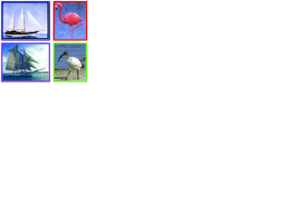
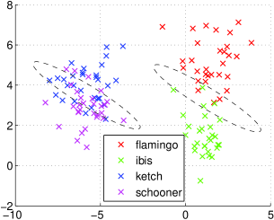
More concretely, the advantage of SL-NE over LMNN can be illustrated through an example shown in Fig. 1 and the corresponding accuracy comparisons listed in Table 1. LMNN can discriminate well between two coarse-grained classes “bird” and “boat”, but fails to learn the subtle differences between fine-grained categories, i.e. “flamingo” vs “ibis” or “ketch” vs “schooner”. This is because a large part of LMNN’s effort is wasted on optimizing unimportant similarity constraints (e.g. “ibis” vs “ketch”), which makes the learning less effective. On the other hand, SL-NE finds the local discriminative structure due to its neighborhood embedding formulation, and achieves much higher accuracies than both kNN with Euclidean distance and LMNN. It is noted that metrics organized in a tree structure [13, 33] have been proposed to learn similarities with varying granularity in an object category hierarchy. SL-NE can pick the most discriminative granularity level and learn a similarity function without any knowledge on object ontology.

The philosophy behind SL-NE is to learn a shared local data structure with information from different neighborhoods complementing each other, which is also used in many other machine learning models. E.g., in Gaussian mixture model and Relevant Component Analysis (RCA) [34], the covariance matrices are tied for all the mixture components or classes; in the localized versions of Neighborhood Component Analysis (NCA) [24, 35] and Fisher Discriminant Analysis (FDA) [36], the importance of a training pair is weighted according to their affinity. It should be noted that in the NCA methods [24, 35], the neighborhood is dynamically updated according to current distance metric. While in SL-NE, the neighborhood is fixed throughout the learning iteration (with neighbors’ ranks being updated), which is more scalable to large data sets.

Besides the performance advantage, it is obvious to see the computational saving of SL-NE over LMNN. The total number of triplet constraints to be considered is on the order of $N^{2}k$ for LMNN which regards all the samples with labels other than $y_{i}$ as the imposters for $\mathbf{x}_{i}$, while only around $Nk^{2}$ for SL-NE which defines similarity exclusively for neighboring samples. Therefore, a significant reduction of computational complexity by a factor of $N/k$ can be achieved for large-scale data with $N{\gg}k$.

3 Ensemble of Distributed Similarities

Recent progress in image classification has witnessed the benefits of building features with very high dimensionality [37]. However, metric learning on such high-dimensional features can be prohibitively expensive. Many methods have tried to learn the metric on a subspace with much lower dimension by imposing a low rank constraint on the distance kernel [11, 7], which, unfortunately, makes the problem non-convex [20]. Although the bilinear similarity function in (2) takes a very simple form, it still has computation complexity quadratic to data dimension. To make our method also scalable to high-dimensional data in terms of computation and data I/O, we propose to use an ensemble of low-dimensional subspace projections so that the learning and evaluation of the similarity function can be conducted in a set of low-dimensional spaces distributedly. Specifically, based on the similarity in (2), we define an ensemble of similarities as

$$s_{E}(\mathbf{x}_{i},\mathbf{x}_{j})=\sum\limits_{n=1}^{N_{E}}s_{\mathbf{M}_{n}}(\mathbf{P}_{n}\mathbf{x}_{i},\mathbf{P}_{n}\mathbf{x}_{j})=\sum\limits_{n=1}^{N_{E}}\mathbf{x}_{i}^{T}\mathbf{P}^{T}_{n}\mathbf{M}_{n}\mathbf{P}_{n}\mathbf{x}_{j},$$ (8)

where $\{\mathbf{P}_{n}\}_{n=1}^{N_{E}}$ is a set of $d{\times}D$ matrices that project data samples $\{\mathbf{x}_{i}\}$ from the original $\mathbb{R}^{D}$ space to $\mathbb{R}^{d}$ spaces, with $d<D$. $N_{E}$ is the number of projections used in the ensemble. $\mathbf{M}_{n}$ is the parameter of the similarity function in the $n$-th projected space. Ideally, $\{\mathbf{P}_{n}\}_{n=1}^{N_{E}}$ should be a set of projections capturing complementary discriminative information. However, learning these discriminative projections can be expensive and thus spoils the algorithm’s scalability. In practice, we find that projections built as consecutive partitions of PCA directions and random projections are both good candidates for $\{\mathbf{P}_{n}\}$. With the additional benefit of knowing the energy in each projection, PCA projections decorrelate the data in different subspaces, which guarantees their complementarity in certain sense. PCA directions can be efficiently approximated using a subset of data, and it entails a one-time computation as opposed to low-rank metric which performs extra calculation in each training iteration, Random projections also have several attractive properties. First, they can be obtained virtually at no cost. Besides, they can well preserve distance in high-dimensional space according to the Johnson-Lindenstrauss lemma [38], as well as low-rank data structure according to [39].

From (8), we can see that learning the similarity function $s_{\mathbf{M}_{n}}$ in the $n$-th projected space is equivalent to learning a similarity function $s_{\mathbf{M}}$ in the original space, with low rank and subspace constraints induced by $\mathbf{P}_{n}$ and imposed on $\mathbf{M}$. From (8), we can further interpret that the ensemble of similarity functions tries to approximate the complete space parameter $\mathbf{M}$ with the summation of a set of parameters $\{\mathbf{M}_{n}\}$ constrained to subspaces.

Ensemble learning of multiple metrics has been explored in literatures with different settings. A local distance metric method is proposed in [14], which learns a metric for each training sample and combines them in the form of class probability prediction. Such an approach is not scalable to large data sets. Boosting algorithms are employed to select and combine multiple weak metrics in [40, 41]. The metrics have to be learned sequentially, which is not efficient when the number of metrics is large. The ensemble method proposed here focuses on parallel learning of multiple metrics. Such computational advantage is also leveraged by the random forest metric [42], which regresses the distance function as the average of binary outputs from a set of decision trees. Another method of ensemble metric learning with parallel capability is introduced in [43], where the ensemble is based on different partitions of class subsets so that better scalability to sample size instead of sample dimension is achieved.

3.1 Learning Algorithm

Learning the ensemble similarity $s_{E}(\cdot,\cdot)$ requires optimizing the objective function in (6) with the similarity defined in (8). Applying SL-NE in Algorithm 1 to find all the $\mathbf{M}_{n}$’s jointly induces a computational complexity of $O(N_{E}{\cdot}d^{2})$, which may not offer too much gain over the original complexity of $O(D^{2})$ if a large ensemble size $N_{E}$ is used. Instead, we propose a Similarity Learning with Distributed Ensemble (SL-DE) algorithm with the computational advantage that each single similarity function in the ensemble can be learned independently in a distributed manner. Given the projection matrix $\mathbf{P}_{n}$, each $\mathbf{M}_{n}$ is learned in parallel in the projected space of $\mathbf{P}_{n}\mathbf{x}$ using SL-NE, which has time complexity $O(d^{2})$. The resulting similarity functions can be directly combined to approximate the optimal ensemble similarity $s_{E}(\cdot,\cdot)$ according to (8). In this way, we can potentially reduce the computational complexity from $O(D^{2})$ to $O(d^{2})$ if not considering the overhead in parallelization. Learning the similarity functions in low-dimensional spaces also helps the optimization converge more quickly, which offers additional saving in computation.

Since the individually learned $\mathbf{M}_{n}$’s are suboptimal, when computation resource allows, we can further carry out an optional step that jointly optimizes them by minimizing the objective in (6). The joint optimization can be done in a coordinate descent manner, where each $\mathbf{M}_{n}$ is sequentially updated with all the others in $s_{E}(\cdot,\cdot)$ fixed. With a reasonable initialization from the individually trained $\mathbf{M}_{n}$’s, this joint optimization does not take long to converge in practice.

Lastly, we want to point out that the idea of SL-DE can be used to accelerate other general metric learning methods and is not limited to SL-NE.

4 Experiments

In this section, we test the performance of the proposed SL-NE learning algorithm and its ensemble version SL-DE on several data sets.

In all the experiments, we use Locality-constrained Linear Coding (LLC) [44] as the image feature. With code book size $2048$ and spatial pyramid matching on the $1{\times}1$, $2{\times}2$ and $4{\times}4$ grids, the LLC feature representation is of $43{,}008$ dimensions. Unless otherwise specified, we project the LLC features to the $3{,}000$ dimensional PCA space and normalize their lengths, which is regarded as the input feature space for all the metric learning methods considered here. For the SL-NE and SL-DE methods, we set margin $b{=}0.02$ and initial step size $\rho_{0}{=}0.2$.The training of SL-DE is performed on a number of distributed nodes in a computer cluster. The local neighborhood $\mathcal{N}_{i}$ is approximately found using an image retrieval system [45] which is efficient for large-scale applications and has a high recall of images from the same class. Note that SL-NE is open to any neighborhood construction method, including approximate nearest neighbor search and hashing. The same neighborhood found in the original feature space is used to learn the similarity of each projected subspace in SL-DE.

Our learned similarity functions are used with a soft-voting kNN classifier to make prediction for test samples, where the voting weight are given by the similarity scores. Specifically, for a test sample $\mathbf{x}_{t}$ whose $k$ nearest training neighbors are indexed by a set $\mathcal{N}_{t}$, its class label can be predicted as:

$$\hat{y}_{t}=\arg\max_{c}\sum\limits_{j\in\mathcal{N}_{t},y_{j}=c}s(\mathbf{x}_{t},\mathbf{x}_{j}).$$ (9)

The voting members for each test sample are selected from its local neighborhood instead of the entire training set so that the testing is also scalable to sample size.

Our SL-NE and SL-DE methods are compared with linear SVM, the Retrieval system [45] which generates the initial neighborhoods, and LMNN [11] whose code is publicly available. A rough comparison on training complexity for all these five methods is given in Table 2. Generally, metric learning methods are more scalable than one-versus-all SVM in terms of the number of classes. Our SL-NE is more scalable than LMNN in terms of the number of training samples due to its neighborhood embedding formulation, and SL-DE further improves over SL-NE on the scalability of data dimension by parallel computation.

Table 2: Training time complexities.

	sample number	class number	data dimension
linear SVM	linear	linear	linear
Retrieval [45]	linear	constant	constant
LMNN [11]	quadratic	constant	quadratic
SL-NE	linear	constant	quadratic
SL-DE	linear	constant	constant (parallel)

In the following, we first analyze in Sec. 4.1 the characteristics of SL-NE and SL-DE algorithms on the small-sized Caltech 101 data set [46]. Then more results of classification on middle-scale and large-scale data are discussed in Sec. 4.2 and 4.3, respectively.

4.1 Algorithm Analysis

Figure 2: Accuracy on test set versus training iterations on the Caltech 101 data using SL-NE.

(a)	(b)
(c)	(d)

Figure 3: (a)$\sim$(d): A test image is shown in the left, and the training images most similar to it is shown in the right, found by Retrieval [45] (top row) and SL-NE (bottom row).

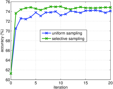
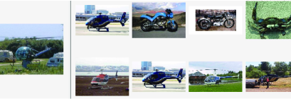
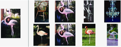
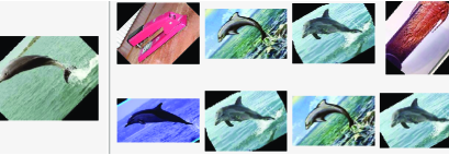
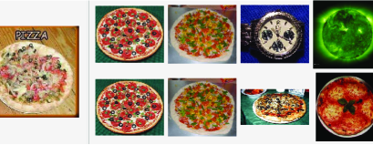
We first examine the optimization behavior for SL-NE algorithm in Fig. 2. Two types of triplet sampling strategy are compared: uniform sampling and the selective sampling defined by (2.1). With either sampling strategy, the performance of the learned similarity function improves a lot over the initial inner product similarity in the original space. Moreover, the proposed selective sampling can converge faster than uniform sampling and attains higher accuracy. Some examples of similar images found by Retrieval and the SL-NE algorithm are shown in Fig. 3. It can be seen that the images found by SL-NE are more semantically similar to the test images and are more likely to come from the same classes.

(a)	(b)

Figure 4: Test accuracy of SL-DE using random projections on the Caltech 101 data: (a) plotted as a function of ensemble size $N_{E}$ for various projected dimension $d$’s; (b) plotted as a function of projected dimension $d$ for $N_{E}=1$ and $N_{E}=20$ similarity function(s) used in ensemble.

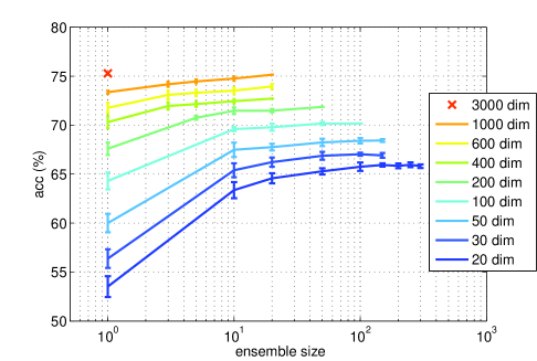
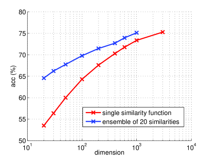
The performance of SL-DE is studied in Fig. 4 with different combinations of projection dimension $d$ and ensemble size $N_{E}$. Here we project image features from the original $3{,}000$ dimensional space to random subspaces of dimensions ranging from $20$ to $1{,}000$. From Fig. 4 (a), we see that the accuracy of SL-DE increases with the size of ensemble, and converges to a certain bound determined by the projection dimension. An ensemble of $10$ similarity functions in $1{,}000$ dimensional projected spaces, for example, can achieve almost the same performance as the single similarity function learned in the original $3{,}000$ dimensional space. The total computation for the two are about the same, but the ensemble approach can be more easily parallelized. It is further observed from (b) that, compared to the single similarity function learned by SL-NE, SL-DE with an ensemble size $20$ can work in subspaces of much reduced dimension without compromise in performance.

4.2 Results on Middle Scale Data

The classification performance of our methods are validated on several benchmark data sets including the Caltech 101 [46] (9,144 images from 102 object classes), the Caltech 256 [47] (30,607 images from 257 object classes) and the SUN [48] (108,754 images from 397 scene categories). We randomly select 30 samples/80 samples/70% samples from each class as training set for the Caltech 101/Caltech 256/SUN data set, respectively. In our SL-NE and SL-DE methods, the local neighborhood size $|\mathcal{N}|$ is chosen as 50/50/500 in both training and testing. The neighborhood size is selected to be about the same as the size of each class in the data sets. For the SL-DE method, an ensemble of similarity functions in 1,000/300/500 dimensional PCA and random subspaces is trained for the three data sets respectively. Note we just choose the ensemble parameters arbitrarily as long as the computation resource allows. The top-1 and top-3 classification accuracies are shown in Table 3, with comparison to several baseline approaches. On all the data sets, our SL-NE method is much better than the unsupervised Retrieval, and most of the time it also outperforms the popular linear SVM classifier by 2$\sim$3%. SL-NE also achieves much higher accuracies than LMNN (which cannot complete in a reasonable amount of time on the SUN set). This indicates that the neighborhood embedding formulation can not only reduce training complexity, but also improve the learning effectiveness by focusing on more relevant data. The accuracies attained by the SL-DE method are very close to those of SL-NE, even though SL-DE are learned based on features projected to subspaces with much lower dimensions. On the SUN data set, SL-DE even performs better than SL-NE, which implies that sometimes directly learning a similarity function in high-dimensional space may not be as effective as the ensemble approach.

Table 3: Top $n$ classification accuracies (%) for middle scale data sets.

Data set	Top-$n$	SVM	Retrieval [45]	LMNN [11]	SL-NE	SL-DE
Caltech 101	1	73.46	63.49	69.16	75.28	75.14
	3	84.59	77.87	80.83	85.29	85.30
Caltech 256	1	43.61	37.28	37.47	46.02	45.39
	3	56.97	48.83	46.84	55.97	55.33
SUN	1	32.08	29.06	–	35.32	35.72
	3	48.73	43.87	–	51.37	52.17

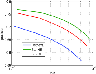
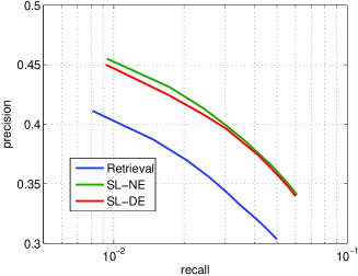
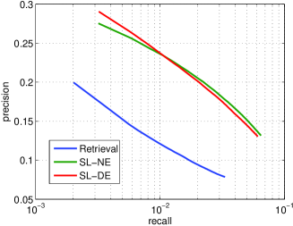
The similarity functions learned by SL-NE and SL-DE can also be regarded as a rerank function for the similar images found by Retrieval. Therefore, we also evaluate their retrieval performance by plotting the precision-recall curves in Fig. 5. SL-NE consistently improves over Retrieval on all the operation points, and SL-DE achieves very similar performance as SL-NE on the Caltech 256 and SUN data sets.

(a) Caltech 101	(b) Caltech 256

(c) SUN

Figure 5: Precision-recall curves for the most similar images found by Retrieval [45], SL-NE and SL-DE.

4.3 Results on Large Scale Data

To further demonstrate the scalability of our methods, we evaluate their performance on the ImageNet Large Scale Visual Recognition Challenge 2010 (ILSVRC’ 10) [8] data set, which contains 1.2M training images from 1,000 object classes, 50K validation images, and 150K test images. On this data set, the first 1,000 PCA dimensions of LLC features are used as our original feature. Neighborhood size $|\mathcal{N}|=500$ is used. The ensemble similarity functions for SL-DE are trained on 10 evenly block-partitioned PCA subspaces, each of 100 dimension. The PCA subspaces are preferred here because a small number of them can give a fair result in relatively short time.

We compare in Table 4 the top-1 flat classification error of the proposed methods with baseline methods including linear SVM, Retrieval, two metric learning based approaches [11, 7], and the average performance on the 10 PCA subspaces using SL-NE. Using the same LLC feature, SL-NE achieves much smaller error rate than Retrieval as well as SVM with an online implementation [49], which implies that similarity learning is more advantageous than one-versus-all classification models on data sets with a huge number of classes. Our SL-NE also improves a lot over LMNN, and has a similar performance as Mensink et al. [7]. It should be noted that Mensink et al. have used fisher vector [37] as their feature representation, which gives an error rate more than 10% lower than what LLC achieves when both are used with a SVM classifier. Therefore, the similarity function learned with SL-NE has made up much of the performance loss due to our weaker feature. Given a better feature representation, our method has the potential to further reduce the classification error.

Table 4: Top-1 flat error rate (%) for ILSVRC’10. Results from [7] are indicated by *.

SVM	Retrieval [45]	LMNN [11]	Mensink et al. [7]	PCA subspace	SL-NE	SL-DE
73.93/60.2*	77.19	72.90*	65.10*	80.44	66.37	68.00

The SL-DE method has a significant improvement over the similarity function learned in each PCA subspace, which serves as its building block. Compared with SL-NE, SL-DE has an error rate less than 2% higher. However, it only takes SL-DE 2 hours (excluding the time to retrieve neighborhood, same below) to train on the 1.2M training set using 10 distributed computers; and this is much faster than SL-NE which needs almost 2 days to complete the same task.

5 Conclusions

A novel image similarity learning method is investigated for better scalability to data set size as well as feature dimensionality. The similarity function is optimized only for sample pairs within a local neighborhood using large margin neighborhood embedding, which significantly reduces the number of relative similarity constraints in training and at the same time enhances the robustness to irrelevant samples. We also propose the ensemble of similarities for scalability to data dimensionality, which breaks the high-dimensional problem into several lower-dimensional problems without much loss in performance. The proposed method is validated on several image classification data sets, and achieves competitive accuracies with several existing methods. More importantly, our approach demonstrates much better scalability than existing metric learning methods and one-versus-all classifiers.

In future work, we will explore other possibilities to find local neighborhoods for better tradeoff between search efficiency and accuracy. Potential directions include using hash functions and joint optimization of neighborhood searching and similarity learning. It is also of great interest to investigate efficient learning of discriminative and complementary projection matrices for ensemble metric learning.

References

- [1] Harchaoui, Z., Douze, M., Paulin, M., Dudik, M., Malick, J.: Large-scale image classification with trace-norm regularization. In: Proc. CVPR. (2012) 3386–3393
- [2] Liu, B., Sadeghi, F., Tappen, M., Shamir, O., Liu, C.: Probabilistic label trees for efficient large scale image classification. In: Proc. CVPR. (2013) 843 – 850
- [3] Li, Q., Wu, J., Tu, Z.: Harvesting mid-level visual concepts from large-scale internet images. In: Proc. CVPR. (2013) 851 – 858
- [4] Tighe, J., Lazebnik, S.: Finding things: Image parsing with regions and per-exemplar detectors. In: Proc. CVPR. (2013) 3001–3008
- [5] Malisiewicz, T., Gupta, A., Efros, A.A.: Ensemble of exemplar-svms for object detection and beyond. In: Proc. ICCV. (2011) 89–96
- [6] Shen, X., Lin, Z., Brandt, J., Wu, Y.: Detecting and aligning faces by image retrieval. In: Proc. CVPR. (2013) 3460–3467
- [7] Mensink, T., Verbeek, J., Perronnin, F., Csurka, G.: Metric learning for large scale image classification: Generalizing to new classes at near-zero cost. In: Proc. ECCV. Springer (2012) 488–501
- [8] Deng, J., Dong, W., Socher, R., Li, L.J., Li, K., Fei-Fei, L.: ImageNet: A large-scale hierarchical image database. In: Proc. CVPR. (2009) 248–255
- [9] Xing, E.P., Jordan, M.I., Russell, S., Ng, A.: Distance metric learning with application to clustering with side-information. In: Advances in Neural Information Processing Systems. (2002) 505–512
- [10] Davis, J.V., Kulis, B., Jain, P., Sra, S., Dhillon, I.S.: Information-theoretic metric learning. In: Proceedings of the 24th International Conference on Machine Learning. (2007) 209–216
- [11] Weinberger, K.Q., Saul, L.K.: Distance metric learning for large margin nearest neighbor classification. J. Mach. Learn. Res. 10 (2009) 207–244
- [12] Law, M.T., Thome, N., Cord, M.: Quadruplet-wise image similarity learning. In: Proc. ICCV. (2013) 249–256
- [13] Hwang, S.J., Sha, F., Grauman, K.: Learning a tree of metrics with disjoint visual features. In: Advances in Neural Information Processing Systems. (2011) 621–629
- [14] Mu, Y., Ding, W., Tao, D.: Local discriminative distance metrics ensemble learning. Pattern Recognition 46 (2013) 2337–2349
- [15] Domeniconi, C., Peng, J., Gunopulos, D.: Locally adaptive metric nearest-neighbor classification. IEEE Trans. PAMI 24 (2002) 1281–1285
- [16] Noh, Y.K., Zhang, B.T., Lee, D.D.: Generative local metric learning for nearest neighbor classification. In: Advances in Neural Information Processing Systems. (2010) 1822–1830
- [17] Wang, J., Kalousis, A., Woznica, A.: Parametric local metric learning for nearest neighbor classification. In: Advances in Neural Information Processing Systems. (2012) 1610–1618
- [18] Hauberg, S., Freifeld, O., Black, M.J.: A geometric take on metric learning. In: Advances in Neural Information Processing Systems. (2012) 2033–2041
- [19] Huang, Y., Li, C., Georgiopoulos, M., Anagnostopoulos, G.C.: Reduced-rank local distance metric learning. In: Machine Learning and Knowledge Discovery in Databases. Springer (2013) 224–239
- [20] Mensink, T., Verbeek, J., Perronnin, F., Csurka, G.: Distance-based image classification: Generalizing to new classes at near-zero cost. IEEE Trans. PAMI 35 (2013) 2624–2637
- [21] Wu, L., Hoi, S.C., Jin, R., Zhu, J., Yu, N.: Learning Bregman distance functions for semi-supervised clustering. IEEE Transactions on Knowledge and Data Engineering 24 (2012) 478–491
- [22] Yan, S., Xu, D., Zhang, B., Zhang, H.J., Yang, Q., Lin, S.: Graph embedding and extensions: a general framework for dimensionality reduction. IEEE Transactions on Pattern Analysis and Machine Intelligence 29 (2007) 40–51
- [23] Zhang, W., Xue, X., Sun, Z., Lu, H., Guo, Y.F.: Metric learning by discriminant neighborhood embedding. Pattern recognition 41 (2008) 2086–2096
- [24] Yang, L., Jin, R., Sukthankar, R., Liu, Y.: An efficient algorithm for local distance metric learning. In: Proceedings of the 21st National Conference on Artificial Intelligence. Volume 1. (2006) 543–548
- [25] Roweis, S.T., Saul, L.K.: Nonlinear dimensionality reduction by locally linear embedding. Science 290 (2000) 2323–2326
- [26] Belkin, M., Niyogi, P.: Laplacian eigenmaps for dimensionality reduction and data representation. Neural computation 15 (2003) 1373–1396
- [27] Chechik, G., Sharma, V., Shalit, U., Bengio, S.: Large scale online learning of image similarity through ranking. The Journal of Machine Learning Research 11 (2010) 1109–1135
- [28] Deng, J., Berg, A.C., Fei-Fei, L.: Hierarchical semantic indexing for large scale image retrieval. In: Proc. CVPR. (2011) 785–792
- [29] Cai, D., He, X., Zhou, K., Han, J., Bao, H.: Locality sensitive discriminant analysis. In: International Joint Conferences on Artificial Intelligence. (2007) 708–713
- [30] Chen, H.T., Chang, H.W., Liu, T.L.: Local discriminant embedding and its variants. In: Proc. CVPR. Volume 2. (2005) 846–853
- [31] Bottou, L.: Large-scale machine learning with stochastic gradient descent. In: Proceedings of COMPSTAT. (2010) 177–186
- [32] Zhu, X.: Semi-supervised learning literature survey. Computer Science, University of Wisconsin-Madison 2 (2006) 3
- [33] Verma, N., Mahajan, D., Sellamanickam, S., Nair, V.: Learning hierarchical similarity metrics. In: Proc. CVPR. (2012) 2280–2287
- [34] Bar-Hillel, A., Hertz, T., Shental, N., Weinshall, D.: Learning distance functions using equivalence relations. In: ICML. Volume 3. (2003) 11–18
- [35] Yang, W., Wang, K., Zuo, W.: Fast neighborhood component analysis. Neurocomputing 83 (2012) 31–37
- [36] Sugiyama, M.: Dimensionality reduction of multimodal labeled data by local fisher discriminant analysis. The Journal of Machine Learning Research 8 (2007) 1027–1061
- [37] Perronnin, F., Sánchez, J., Mensink, T.: Improving the fisher kernel for large-scale image classification. In: Proc. ECCV. (2010) 143–156
- [38] Johnson, W.B., Lindenstrauss, J.: Extensions of lipschitz mappings into a hilbert space. Contemp. Math. 26 (1984) 189–206
- [39] Halko, N., Martinsson, P.G., Tropp, J.A.: Finding structure with randomness: Probabilistic algorithms for constructing approximate matrix decompositions. SIAM review 53 (2011) 217–288
- [40] Huang, C., Zhu, S., Yu, K.: Large-scale strongly supervised ensemble metric learning (2013) US Patent 20,130,129,202.
- [41] Kedem, D., Tyree, S., Weinberger, K., Sha, F., Lanckriet, G.: Non-linear metric learning. In: Advances in Neural Information Processing Systems. (2012) 2582–2590
- [42] Xiong, C., Johnson, D., Xu, R., Corso, J.J.: Random forests for metric learning with implicit pairwise position dependence. In: Proceedings of the 18th ACM SIGKDD international conference on Knowledge discovery and data mining. (2012) 958–966
- [43] Kozakaya, T., Ito, S., Kubota, S.: Random ensemble metrics for object recognition. In: Proc. ICCV. (2011) 1959–1966
- [44] Wang, J., Yang, J., Yu, K., Lv, F., Huang, T., Gong, Y.: Locality-constrained linear coding for image classification. In: Proc. CVPR. (2010) 3360–3367
- [45] Shen, X., Lin, Z., Brandt, J., Avidan, S., Wu, Y.: Object retrieval and localization with spatially-constrained similarity measure and k-NN re-ranking. In: Proc. CVPR. (2012) 3013–3020
- [46] Fei-Fei, L., Fergus, R., Perona, P.: Learning generative visual models from few training examples: An incremental bayesian approach tested on 101 object categories. Computer Vision and Image Understanding 106 (2007) 59–70
- [47] Griffin, G., Holub, A., Perona, P.: Caltech-256 object category dataset. CIT Technical Report (2007)
- [48] Xiao, J., Hays, J., Ehinger, K.A., Oliva, A., Torralba, A.: Sun database: Large-scale scene recognition from abbey to zoo. In: Proc. CVPR. (2010) 3485–3492
- [49] Bottou, L.: Stochastic gradient descent package (version 2) (2011) http://leon.bottou.org/projects/sgd.