Beating pattern in quantum magnetotransport coefficients of spin-orbit coupled Dirac fermions in gated silicene

Abstract

We report theoretical study of magnetotransport coefficients of spin-orbit coupled gated silicene in presence and absence of spatial periodic modulation. The combined effect of spin-orbit coupling and perpendicular electric field manifests through formation of regular beating pattern in Weiss and SdH oscillations. Analytical results, in addition to the numerical results, of the beating pattern formation are provided. The analytical results yield a beating condition which will be useful to determine the spin-orbit coupling constant by simply counting the number of oscillation between any two successive nodes. Moreover, the numerical results of modulation effect on collisional and Hall conductivities are presented.

I INTRODUCTION

Silicene, a new class of two-dimensional (2D) electron system, possess graphene-like hexagonal lattice structure except the atoms are silicon instead of carbontakeda ; guzman . Several experiments of synthesizing monolayer silicene have been performed successfully lalmi ; padova1 ; padova2 ; vogt ; lin ; PRL12 . Relatively larger atomic size of silicon atom causes the 2D lattice to be buckled, in which two planes of sublattice $A$ and sublattice $B$ are separated by $d\backsimeq 0.46\mathring{A}$drummond ; nano . Theoretical investigationsdrummond ; liu1 ; liu2 show that silicene possess an intrinsic spin-orbit coupling which is very strong in comparison to graphene. This is due to the fact that Si atoms have large intrinsic spin-orbit coupling strength than C atoms. The application of electric field ($E_{z}$) perpendicular to the buckled silicene sheet generates a staggered sublattice potential difference ($\Delta_{z}=E_{z}d$) between the two atomic planes and opens an electric field dependent band gap between conduction and valence bands drummond ; ni ; ezawa . The charge carriers in silicene also obey Dirac-like Hamiltonianvogt around the corners of its hexagonal Brillouin zone with additional properties of having intrinsic spin-orbit coupling and electrically tunable band gapdrummond . Moreover, the low-energy dispersion around $K$ and $K^{\prime}$ points splits into two branches due to presence of the both spin-orbit coupling and $\Delta_{z}$. Monolayer graphene’s zero band gap with the difficulty in tuning it and vanishingly small spin-orbit interaction prevent it to be used for electronic devices. On the other hand, silicene overcomes all these limitations and provide an alternative to graphene for device based applications. Recently, a series of theoretical works on transport and optical properties of silicene have been reported, revealing the roles of finite band gap and spin-orbit interactionezawa1 ; tahir_13 ; sabeeh_13 ; nicole ; nicole1 .

The study of magnetotransport coefficients is one of the basic tools to investigate various two-dimensional electron systems. Appearance of quantum oscillation in magnetotransport coefficients, known as Shubnikov-de Hass(SdH) oscillation, is due to the interplay between Landau levels and Fermi energy. A different kind of quantum oscillation, known as Weiss oscillation, appears in magnetoresistance when an in-plane weak spatial electric modulation is applied Weiss ; Gerh ; kotha . The Weiss oscillation is due to the commensurability of the diameter of the cyclotron orbit near the Fermi energy and the spatial period of the modulation poulo ; chao ; vasilo ; beenakker . Both the oscillations are periodic with inverse magnetic field. The Weiss oscillation appears at very low magnetic field where SdH oscillations are completely wiped out. On the other hand, at moderate magnetic field, very weak Weiss oscillation is superposed on the SdH oscillations.

The spin-orbit interaction lifts the spin degeneracy and produces two unequally spaced Landau levels for spin-up and spin-down electrons in a two-dimensional electron gas formed at semiconductor heterostructures. The difference between two frequencies of quantum oscillation for spin-up and spin-down electrons is directly related to the spin-orbit coupling constant and yields beating pattern in the amplitude of the Weiss and SdH oscillations das ; nitta ; wang ; firoz1 ; vasilo1 ; firoz2 . The beating pattern in the SdH oscillations is being used to determine the spin-orbit coupling constant. It is proposed that the beating pattern in Weiss oscillation can be also used to determine spin-orbit coupling constant firoz2 .

The SdH oscillation in graphene monolayer describing by massless Dirac-like Hamiltonian has been experimentally sdh_g ; tahir. The appearance of Weiss oscillation in graphene monolayer has been predicted in Refs. matulis ; tahir1 . The beating pattern in magnetotransport coefficients of graphene monolayer does not appear due to absent of spin-split Landau energy levels. On the other hand, spin-split Landau levels appear in spin-orbit coupled Dirac fermions in gated silicene. There are several theoretical group estimated $\Delta_{\rm so}$ and $\Delta_{z}$ using tight-binding and density functional calculations. In this paper we discuss that $\Delta_{\rm so}$ and $\Delta_{z}$ can be determined experimentally by analyzing beating pattern in magnetotransport coefficients in spin-orbit coupled gated silicene in presence and absence of the spatial periodic modulation.

This paper is arranged in following order. In section II, we present energy eigenvalues, the corresponding eigenstates and density of states of the charge carriers in silicene sheet subjected to transverse magnetic and electric fields. In section III, we present analytical and numerical results of diffusive, collisional and Hall conductivities in presence and absence of the periodic modulation. In section IV we summarize our results.

II ENERGY EIGENVALUE AND EIGENFUNCTION

We are considering a buckled 2D silicene sheet in which Dirac electrons obey a finite gapped graphene-like Hamiltonian. The Hamiltonian of an electron with charge $-e$ in presence of both field, the perpendicular magnetic field ${\bf B}$ and electric field ${\bf E}=E_{z}\hat{z}$, isliu2 ; ezawa1

$$H=v_{F}(\sigma_{x}\Pi_{x}-\eta\sigma_{y}\Pi_{y})-\eta s\Delta_{\rm so}\sigma_{z}+\Delta_{z}\sigma_{z},$$ (1)

where $v_{F}$ is the Fermi velocity, ${\bf\Pi}={\bf p}+e{\bf A}$ is the 2D momentum operator with vector potential ${\bf A}$, $\eta=+(-)$ denotes $K(K^{\prime})$ Dirac point, $s=\pm$ stands for spin-up and spin-down, ${\mbox{\boldmath$\sigma$}}=(\sigma_{x},\sigma_{y},\sigma_{z})$ are the Pauli matrices, $\Delta_{\rm so}$ is the strength of the spin-orbit interaction, and $\Delta_{z}$ is the energy associated with the applied electric field.

Using Landau gauge ${\bf A}=(0,Bx,0)$, the exact Landau levels and the corresponding wave functions are obtained in Refs. tahir_13 ; nicole . The ground state energy ($n=0$) is $E_{0}^{\eta}=-(s\Delta_{\rm so}-\eta\Delta_{z})$. For $n\geq 1$, energy spectrum for the electron band is

$$E_{\zeta}=\sqrt{n\varepsilon^{2}+(\Delta_{\rm so}-\eta s\Delta_{z})^{2}},$$ (2)

where $\zeta\equiv\{n,s,\eta\}$, $\varepsilon=\hbar\omega_{c}$ and $\omega_{c}=\sqrt{2}v_{F}/l$ is the cyclotron frequency with $l=\sqrt{\hbar/eB}$ is the magnetic length scale. The Landau levels around $K$ and $K^{\prime}$ points split into two branches due to presence of both $\Delta_{\rm so}$ and $\Delta_{z}$. The splitting vanishes when either $\Delta_{\rm so}$ or $\Delta_{z}$ is zero. The normalized eigenstates are (for $n\geq 1$)

$$\Psi^{\eta=+}_{n,s}({\bf r})=\frac{e^{ik_{y}y}}{\sqrt{L_{y}N_{n,s}^{\eta}}}\left[\begin{array}[]{r}\alpha_{n,s}^{+}\phi_{n-1}(x+x_{0})\\ \beta_{n}\phi_{n}(x+x_{0})\end{array}\right]\text{}$$ (3)

and

$$\Psi^{\eta=-}_{n,s}({\bf r})=\frac{e^{ik_{y}y}}{\sqrt{L_{y}N_{n,s}^{\eta}}}\left[\begin{array}[]{r}\alpha^{-}_{n,s}\phi_{n}(x+x_{0})\\ \beta_{n}\phi_{n-1}(x+x_{0})\end{array}\right]\text{,}$$ (4)

where $\phi_{n}(x)=(1/\sqrt{\sqrt{\pi}2^{n}n!l})e^{-x^{2}/2l^{2}}H_{n}(x/l)$ is the normalized harmonic oscillator wave function centred at $x=-x_{0}$ with $x_{0}=k_{y}l^{2}$. Here, the coefficients are $N_{n,s}^{\eta}=\mid\alpha_{n,s}^{\eta}\mid^{2}+\mid\beta_{n}\mid^{2}$ with $\alpha^{\eta}_{n,s}=\Delta_{\eta,s}+\sqrt{\Delta_{\eta,s}^{2}+n(\hbar\omega_{c})^{2}}$ and $\beta_{n}=-i\hbar\omega_{c}\sqrt{n}$. Here, $\Delta_{\eta,s}=(\Delta_{\rm so}-\eta s\Delta_{z})$.

The analytical form of density of states dos is given by

$$D_{\eta,s}(E) \backsimeq D_{0}(E)\Big{[}1+2\sum_{k=1}^{\infty}\exp\Big{\{}-k\Big{(}2\pi\frac{\Gamma_{0}E}{\varepsilon^{2}}\Big{)}^{2}\Big{\}}$$ (5)

$$\times \cos\Big{\{}\pi s\Big{(}E^{2}-\Delta_{\eta,s}^{2}\Big{)}/\varepsilon^{2}\Big{\}}\Big{]},$$

where $D_{0}(E)=E/(2\pi\hbar^{2}v_{F}^{2})$ and $\Gamma_{0}$ is the impurity induced Landau level broadening.

III Electrical Magnetotransport

In this section we shall study magnetotransport coefficients such as diffusive, collisional and Hall conductivities. The diffusive conductivity in absence of any modulation exactly vanishes because of the zero group velocity due to $k_{y}$ degeneracy in the energy spectrum. The presence of modulation imparts drift velocity to the charge carriers along the free direction of it’s motion and gives rise to diffusive conductivity. The oscillations in the diffusive conductivity known as Weiss oscillation which is dominant at low magnetic field regime. On the other hand, the collisional conductivity arises due to scattering of the charge carriers with localized charged impurities present in the system. The quantum oscillation in collisional conductivity is known as SdH oscillation. The Hall conductivity due to the Lorentz force is independent of any collisional mechanisms. However, the external spatial periodic modulation induces periodic oscillation on collisional as well as Hall conductivities. We shall use formalism of calculating different magnetotransport coefficients developed in Ref. vilet .

III.1 Diffusive conductivity

To study diffusive conductivity, a spatial weak electrical modulation $V=V_{0}\cos(Kx)$ with $K=2\pi/a$ is applied along the $x$ direction of the silicene sheet. Here, $a$ is the modulation period. We can treat this modulation as a weak perturbation as long as $V_{0}\ll\epsilon$. The energy correction due to the modulation is calculated approximately by using first-order perturbation theory. Then total energy is given by $E_{\xi}=E_{\zeta}+\Delta E_{\xi}$, where $\xi\equiv\{\zeta,k_{y}\}$ and $\Delta E_{\xi}=G_{\zeta}(u)\cos(Kx_{0})$ with

$$G_{\zeta}(u)=\frac{V_{0}e^{-u/2}}{N_{n,s}^{\eta}}\Big{[}\mid\alpha_{n,s}^{\eta}\mid^{2}L_{n-1}(u)+\mid\beta_{n}\mid^{2}L_{n}(u)\Big{]}.$$ (6)

Here, $u=(Kl)^{2}/2$ and $L_{n}(u)$ is the Laguerre polynomial of degree $n$. The energy correction $\Delta E_{\xi}$ transforms the degenerate Landau levels into bands due to $k_{y}$ dependency, which leads to non-zero drift velocity.

The diffusive conductivity is calculated by using the standard semiclassical expression as

$$\sigma_{yy}^{\rm dif}=\frac{\beta e^{2}\tau}{\Omega}\sum_{\xi}f_{\xi}(1-f_{\xi})(v_{y}^{\xi})^{2},$$ (7)

where $\Omega=L_{x}\times L_{y}$ is the area of the system, $\tau=\tau(E_{F})$ is the electron relaxation time at the Fermi energy $E_{F}$ which is calculated in the next paragraph, $f_{\xi}$ is the Fermi-Dirac distribution function at $E=E_{\xi}$ and $\beta=(k_{B}T)^{-1}$ with $k_{B}$ is the Boltzmann constant. Also, $v_{y}^{\xi}=\langle\xi|\hat{v}_{y}|\xi\rangle$ is the average value of the velocity operator $\hat{v}_{y}$ and it does not vanish due to the $k_{y}$ dependency of the energy levels. It is given by

$$v_{y}^{\xi}=\frac{1}{\hbar}\frac{\partial E_{\xi}}{\partial k_{y}}=-\frac{Kl^{2}}{\hbar}\sin(Kx_{0})G_{\zeta}(u).$$ (8)

After inserting drift velocity given by Eq. (8) into Eq. (7) and integrating over $k_{y}$ variable, we get $\sigma_{yy}^{\rm dif}=(e^{2}/h)\Phi$ with

$$\Phi=\frac{\beta\tau u}{\hbar}\sum_{\zeta}f(E_{n,s}^{\eta})[1-f(E_{n,s}^{\eta})][G_{\zeta}(u)]^{2}$$ (9)

is the dimensionless total diffusive conductivity. Note that a given Landau level splits into two branches due to the simultaneous presence of $\Delta_{\rm so}$ and $\Delta_{z}$. The first branch is $E_{n}^{-}=\sqrt{n\varepsilon^{2}+(\Delta_{\rm so}-\Delta_{z})^{2}}$ for $\{s,\eta\}=\{+,+\}$ and $\{-,-\}$. The second branch is $E_{n}^{+}=\sqrt{n\varepsilon^{2}+(\Delta_{\rm so}+\Delta_{z})^{2}}$ for $\{s,\eta\}=\{+,-\}$ and $\{-,+\}$. So, for $\eta=+1$ ($K$-valley) there are two energy branches due to spin splitting and same goes for $\eta=-1$ ($K^{\prime}$-valley) also. The total conductivity is written as $\Phi=\Phi^{+}+\Phi^{-}$. Here, $\Phi^{+}$ is the contribution from the second branch $E_{n}^{+}$ and $\Phi^{-}$ is coming from the first branch $E_{n}^{-}$.

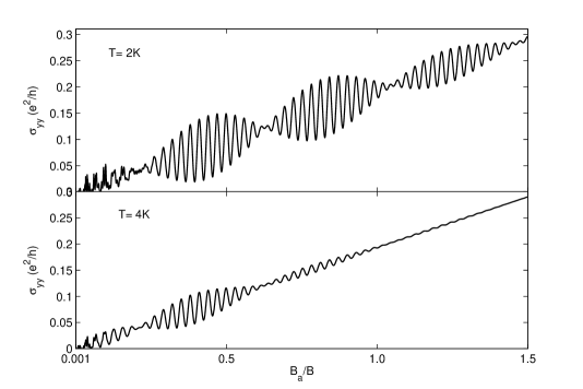
Figure 1: Plots of the exact results of the diffusive conductivity versus dimensionless inverse magnetic field $\lambda$.

Before simplifying further, we shall derive the Fermi energy. At Fermi level $E_{F}=\sqrt{(\hbar v_{F}k_{F}^{\pm})^{2}+\Delta^{2}_{\pm}}$ with $\Delta_{\pm}=(\Delta_{\rm so}\mp\Delta_{z})$, then one can write

$$(k_{F}^{+})^{2}-(k_{F}^{-})^{2}=4\frac{\Delta_{\rm so}\Delta_{z}}{(\hbar v_{F})^{2}}.$$ (10)

On the other hand, carrier density is given by

$$n_{e}=\frac{2}{(2\pi)^{2}}\int_{0}^{2\pi}\int_{0}^{k_{F}}kdkd\phi=\frac{1}{2\pi}\Big{[}(k_{F}^{+})^{2}+(k_{F}^{-})^{2}\Big{]}.$$ (11)

Solving the above two equations for Fermi energy, we get $E_{F}=\sqrt{(E_{F}^{0})^{2}+\Delta_{\rm so}^{2}+\Delta_{z}^{2}}$ with $E_{F}^{0}=\hbar v_{F}k_{F}^{0}$ and $k_{F}^{0}=\sqrt{\pi n_{e}}$.

Before presenting exact analytical results, we would like to get approximated analytical results. To do so we consider the system at very low temperature in which Landau levels close to the Fermi energy contribute to transport properties. Therefore, we can use some approximations which are valid for higher values of $n$. Around Fermi level, for higher value of $n$, we have

$$e^{-u/2}L_{n}(u)\simeq\frac{1}{\sqrt{\pi\sqrt{nu}}}\cos\Big{(}2\sqrt{nu}-\pi/4\Big{)}.$$ (12)

We can also use $n\backsimeq n-1$ for higher values of Landau levels, which give $G_{\zeta}(u)\simeq V_{0}\exp(-u/2)L_{n}(u)$. To obtain analytical expression we convert the summation into integration by using the relation

$$\sum_{n}\rightarrow\int_{0}^{\infty}dn\simeq\frac{2}{\varepsilon^{2}}\int_{0}^{\infty}EdE.$$ (13)

By using the above two approximations, the exact expression of the dimensionless diffusive conductivity given by Eq. (9) reduces to

$$\Phi^{\pm} \backsimeq A_{0}\frac{u}{c^{\pm}}\int_{-\infty}^{\infty}\frac{\cos^{2}(c^{\pm}t+d^{\pm})}{\cosh^{2}(t/2)}dt,$$

where $A_{0}=V_{0}^{2}\tau_{0}/(\hbar\beta\varepsilon^{2})$, $t=\beta(E-E_{F})$, and $d^{\pm}=c^{\pm}\beta E_{F}$ with

$$c^{\pm}=\frac{2\sqrt{u}}{\varepsilon}\frac{\sqrt{(E_{F}^{0})^{2}\mp 2\Delta_{\rm so}\Delta_{z}}}{\beta E_{F}}.$$ (15)

Using the standard integral inti , Eq. (III.1) reduces to

$$\Phi^{\pm}=A_{0}\frac{u}{c^{\pm}}\Big{[}1+H\Big{(}T/T_{a}^{\pm}\Big{)}\cos\Big{(}2\pi f^{\pm}\lambda\Big{)}\Big{]}.$$ (16)

Here, $\lambda=B_{a}/B$ with $B_{a}=\hbar/ea^{2}$ and

$$f^{\pm}=\frac{2a}{\hbar v_{F}}\sqrt{(E_{F}^{0})^{2}\mp 2\Delta_{\rm so}\Delta_{z}}$$ (17)

are two closely spaced frequencies of Weiss oscillations of the two energy branches induced by the simultaneous presence of spin-orbit interaction and gate induced electric field. The temperature dependent damping factor is given by

$$H\Big{(}T/T_{a}^{\pm}\Big{)} = \frac{T/T_{a}^{\pm}}{\sinh(T/T_{a}^{\pm})},$$

where the characteristic temperature $(T_{a}^{\pm})$ is defined as

$$T_{a}^{\pm}=\hbar v_{F}E_{F}B/\Big{[}4\pi^{2}k_{B}aB_{a}\sqrt{(E_{F}^{0})^{2}\mp 2\Delta_{\rm so}\Delta_{z}}\Big{]}.$$ (18)

Typically the difference between $T_{a}^{+}$ and $T_{a}^{-}$ is very small. $T_{a}^{-}=0.76$ K when $B=0.6$ T. Another point is that $T_{a}^{+}$ is increasing with electric field ($\Delta_{z}$) or spin-orbit interaction ($\Delta_{\rm so}$) while $T_{a}^{-}$ is decreasing.

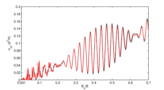
Figure 2: Plots of the exact and analytical results of diffusive conductivity versus dimensionless inverse magnetic field. The dark and red lines stand for analytic and numerical results.

As $(E_{F}^{0})^{2}\gg 2\Delta_{\rm so}\Delta_{z}$, the total diffusive conductivity is given by

$$\Phi\backsimeq 2A_{0}\frac{u}{c}\big{[}1+H\big{(}T/T_{a}\big{)}\cos(2\pi f_{\rm av}\lambda)\cos(2\pi f_{d}\lambda)\big{]}$$ (19)

with $c=2\sqrt{u}E_{F0}/(\beta E_{F})$, $T_{a}=\hbar v_{F}E_{F}B/(4\pi^{2}k_{B}aB_{a}E_{F}^{0})$, $f_{\rm av}=(f^{+}+f^{-})/2$ and $f_{d}=(f^{+}-f^{-})/2$. The total diffusive conductivity given by Eq. (19) exhibits beating pattern due to the superposition of two oscillatory functions with closely spaced frequencies $f^{\pm}$. It should be noted that the condition $(E_{F}^{0})^{2}>2\Delta_{\rm so}\Delta_{z}$ must be satisfied to see the beating pattern. The location of the beating node can be obtained from the condition $\cos(2\pi f_{d}\lambda)\mid_{{}_{B=B_{j}}}=0$, which gives

$$2f_{d}\frac{B_{a}}{B_{j}}=\Big{(}j+\frac{1}{2}\Big{)},$$ (20)

where $j=0,1,2...$. Another periodic term, $\cos(2\pi f_{\rm av}\lambda)$, gives number of oscillation between two successive beating nodes as

$$N_{\rm osc}=f_{\rm av}\Big{(}\frac{B_{a}}{B_{j+1}}-\frac{B_{a}}{B_{j}}\Big{)}=\frac{1}{2}\frac{f_{\rm av}}{f_{d}}.$$ (21)

In explicit form, it is given by

$$2N_{\rm osc}=\frac{\sqrt{(E_{F}^{0})^{2}+2\Delta_{\rm so}\Delta_{z}}+\sqrt{(E_{F}^{0})^{2}-2\Delta_{\rm so}\Delta_{z}}}{\sqrt{(E_{F}^{0})^{2}+2\Delta_{\rm so}\Delta_{z}}-\sqrt{(E_{F}^{0})^{2}-2\Delta_{\rm so}\Delta_{z}}}.$$ (22)

Here we make couple of important remarks on the above equation: 1) number of oscillation between any two successive beat nodes is independent of the modulation period $a$ and magnetic field and 2) the expression of $N_{\rm osc}$ can be used to estimate the spin-orbit coupling constant by simply counting the number of oscillations between any two successive beat nodes.

We use the following parameters for various plots: electron density $n_{e}=4\times 10^{15}$m^-2, spin-orbit coupling constant $\Delta_{\rm so}=4$ meV, perpendicular electric field induced energy $\Delta_{z}=12$ meV, Fermi velocity $v_{F}=2\times 10^{5}$ ms^-1, modulation period $a=150$ nm, and modulation strength $V_{0}=0.1$ meV. Figure 1 shows exact numerical results of the diffusive conductivity given by Eqs. (7) and (8) for two different temperature. It shows beating pattern in both the cases, and oscillation gets damped with increasing temperature. In Fig. 2 we compare the approximate analytical result given by Eq. (19) with the exact numerical result obtained from Eq. (7). The analytical result for diffusive conductivity matches very well with the exact result. The appearance of beating pattern is due to the superposition of Weiss oscillation coming from two oscillatory drift velocity with different frequencies ($f^{\pm}$) corresponding to two energy branches. For the numerical parameters used here, the number of oscillations calculated from Eq. (22) is 14, same as counted from Fig. 1.

III.2 Collisional Conductivity

First we shall study collisional conductivity in absence of modulation. The effect of modulation on SdH oscillation will be discussed in the later half of this section. The standard expression for collisional conductivity is given byvilet

$$\sigma_{\mu\mu}^{\rm col}=\frac{\beta e^{2}}{2\Omega}\sum_{\zeta,\zeta^{\prime}}f_{\zeta}(1-f_{\zeta^{\prime}})W_{\zeta,\zeta^{\prime}}(\alpha_{\mu}^{\zeta}-\alpha_{\mu}^{\zeta^{\prime}})^{2}.$$ (23)

Here, $f_{\zeta}=f_{\zeta^{\prime}}$ for elastic scattering, $W_{\zeta,\zeta^{\prime}}$ is the transition probability between one-electron states $|\zeta\rangle$ and $|\zeta^{\prime}\rangle$. Also, $\alpha_{\mu}^{\zeta}=\langle\zeta|r_{\mu}|\zeta\rangle$ is the average value of $\mu$ component of the position operator of the charge carriers in state $|\zeta\rangle$. The scattering rate $W_{\zeta,\zeta^{\prime}}$ is given by

$$W_{\zeta,\zeta^{\prime}}=\sum_{{\bf q}}|U({\bf q})|^{2}|\langle\zeta|e^{i{\bf q}\cdot({\bf r}-{\bf R})}|\zeta^{\prime}\rangle|^{2}\delta(E_{\zeta}-E_{\zeta^{\prime}}),$$ (24)

where ${\bf q}=q_{{}_{x}}\hat{x}+q_{{}_{y}}\hat{y}$ is the two-dimensional wave-vector and $U({\bf q})=2\pi e^{2}/(\epsilon\sqrt{q_{{}_{x}}^{2}+q_{{}_{y}}^{2}+k_{s}^{2}})$ is the Fourier transform of the screened impurity potential $U({\bf r})=(e^{2}/4\pi\epsilon)(e^{-k_{s}r}/r)$, where $k_{s}$ is the inverse screening length and $\epsilon$ is the dielectric constant of the material. Equation (23) can be re-written for higher values of Landau level ($n\backsimeq n-1$) as given by

$$\sigma_{xx}^{\rm col}=\frac{e^{2}}{h}\frac{N_{I}U_{0}^{2}}{\pi l^{2}\Gamma_{0}}\sum_{\zeta}(2n+1)\Big{[}-\frac{\partial f}{\partial E}\Big{]}_{E=E_{\zeta}}.$$ (25)

A closed-form analytical expression of the above equation is obtained by replacing the summation over quantum number as $\sum_{n}\rightarrow 2\pi l^{2}\int_{0}^{\infty}D(E)dE$ with $D(E)$ is the density of states (see Eq. (5)) and it is given by

$$\sigma_{xx}^{\rm col(\pm)} \backsimeq \frac{\sigma_{0}}{(\omega_{c}\tau_{0})^{2}}\frac{E_{F}^{2}-\Delta_{\pm}^{2}}{\varepsilon^{2}}$$ (26)

$$\times \Big{[}1+2\Omega_{D}H\Big{(}T/T_{c}\Big{)}\cos\Big{(}2\pi\nu^{\pm}/B\Big{)}\Big{]}.$$

Here, $\sigma_{0}=e^{2}\tau_{0}E_{F}/\pi\hbar^{2}$ is Drude-like conductivity and $\nu^{\pm}=[(E_{F}^{0})^{2}\pm 2\Delta_{z}\Delta_{\rm so}]/(2e\hbar v_{F}^{2})$ are the SdH oscillation frequencies for the two energy branches $E_{n}^{+}$ and $E_{n}^{-}$. Also, impurity induced damping factor is

$$\Omega_{D}=\exp\Big{\{}-\Big{(}2\pi\frac{\Gamma_{0}E_{F}}{\varepsilon^{2}}\Big{)}^{2}\Big{\}}$$ (27)

and the temperature dependent damping factor is $H(x)=x/\sinh(x)$. Here, $x=T/T_{c}$ with $T_{c}=\varepsilon^{2}/(2\pi^{2}k_{B}E_{F})$ is the critical temperature.

Following the same procedure as in the diffusive conductivity case, here we get the location of a beating node ($B_{j}$) as $B_{j}(j+1/2)=2\Delta_{\rm so}\Delta_{z}/(e\hbar v_{F}^{2})$ and number of oscillations between any two successive nodes as $N_{\rm osc}^{\rm s}=(E_{F}^{0})^{2}/(4\Delta_{\rm so}\Delta_{z})$. Unlike Rashba spin-orbit coupled two-dimensional electron gas, $N_{\rm osc}^{s}$ in silicene is same for a set of given parameters and does not depend on specific choices of the successive nodes. In Fig. 3, we show the beating pattern in the collisional conductivity vs inverse magnetic field. For the parameters used here, we have $N_{\rm osc}^{s}=14$ which is same as shown in Fig. 3.

Figure 3: Plots of the exact and analytical results of the collisional conductivity versus inverse magnetic field in absence of modulation. Here, red and dark lines stand for numeric and analytic results, respectively.

Now we will describe effect of of weak modulation on the collisional conductivity. The modulation effect enters mainly through the total energy in Fermi distribution function. The collisional conductivity in presence of weak modulation is given by

$$\sigma_{xx}^{\rm col}\backsimeq\frac{e^{2}}{h}\frac{N_{I}U_{0}^{2}}{\pi a\Gamma_{0}}\sum_{\zeta}(2n+1)M_{\zeta},$$ (28)

where $M_{\zeta}$ is given by

$$M_{\zeta} = \int_{0}^{a/l^{2}}\Big{[}-\frac{\partial f}{\partial E}\Big{]}_{E=E_{\xi}}dk_{y}.$$ (29)

It is difficult to get a closed-form analytical expression of the collisional conductivity in presence of the modulation. The change in collisional conductivity due to the modulation [$\Delta\sigma_{xx}^{\rm coll}=\sigma_{xx}^{\rm coll}(V_{0})-\sigma_{xx}^{\rm coll}(0)]$ is calculated from Eq. (28) numerically and shown in Fig. 4.

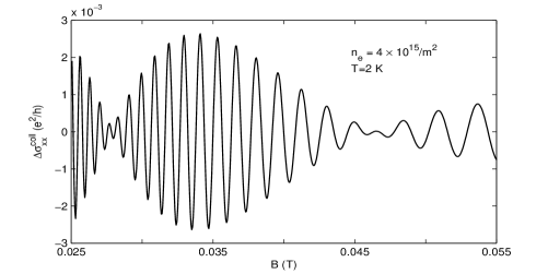
Figure 4: Plots of change in the collisional conductivity due to modulation versus magnetic field.

Figures (3) and (4) clearly shows that effect of the modulation on $\sigma_{xx}^{\rm coll}$ is very small and vanishes with increasing $B$. The location of the beating node and number of oscillations between any two successive nodes are determined by Eqs. (20) and (21), respectively. To understand why the beating pattern appears in $\Delta\sigma_{xx}^{\rm coll}$ follows the same condition as in the diffusive conductivity, we expand $M_{\zeta}$ as given by

$$M_{\zeta} = \int_{0}^{a/l^{2}}\Big{[}\Big{(}-\frac{\partial f}{\partial E}\Big{)}+\Delta E_{\zeta,k_{y}}\Big{(}-\frac{\partial f^{\prime}}{\partial E}\Big{)}$$ (30)

$$+ \frac{(\Delta E_{\zeta,k_{y}})^{2}}{2!}\Big{(}-\frac{\partial f^{\prime\prime}}{\partial E}\Big{)}+.....\Big{]}_{E=E_{\zeta,k_{y}}}dk_{y}$$

$$= \frac{a}{l^{2}}\Big{[}\Big{(}-\frac{\partial f}{\partial E}\Big{)}+\frac{\{G_{\zeta}(u)\}^{2}}{4}\Big{(}-\frac{\partial f^{\prime\prime}}{\partial E}\Big{)}...\Big{]}_{E=E_{\zeta}}.$$

We can see the modulation dependent dominant term is of the order of $(G_{\zeta}(u))^{2}\simeq V_{0}^{2}$, which is same as in the diffusive conductivity (see Eq. 9). The modulation induced Weiss oscillation in collisional conductivity, as shown in Fig. 4., also follows the same beating condition as in the diffusive conductivity.

From the numerical result we can see that modulation effect is dominant at low range of magnetic field i.e; when the energy scale of Landau level is not much higher than the energy correction due to modulation. As magnetic field increases, SdH oscillation starts to dominate over Weiss oscillation.

III.3 The Hall conductivity

In this sub section, we will see modulation effect on the Hall conductivity. The Hall conductivity is given by vilet

$$\sigma_{yx} = \frac{ie^{2}\hbar}{\Omega}\sum_{\xi}\frac{f_{\xi}-f_{\xi^{\prime}}}{{(E_{\xi}-E_{\xi^{\prime}})^{2}}}\langle\xi|\hat{v}_{y}|\xi^{\prime}\rangle\langle\xi^{\prime}|\hat{v}_{x}|\xi\rangle.$$ (31)

Figure 5: Plots of the modulation effect on Hall conductivity versus magnetic field.

Using unperturbed eigenstates velocity matrix elements are given by

$$<n,s,+\mid\hat{v}_{x}\mid n+1,s,+>=\frac{\alpha_{n+1,s}^{+}\beta_{n}}{N_{n+1,s}^{+}N_{n,s}^{+}}v_{F}$$ (32)

and

$$<n+1,s,+\mid\hat{v}_{y}\mid n,s,+>=-i\frac{\alpha_{n+1,s}^{+}\beta_{n}}{N_{n+1,s}^{+}N_{n,s}^{+}}v_{F}.$$ (33)

Substituting Eqs. (32) and (33) into Eq. (31), we get

$$\sigma_{yx} = 2\frac{e^{2}}{h}\frac{l^{2}}{a}\sum_{n,s}\int_{0}^{a/{l}^{2}}\frac{\mid\alpha_{n+1,s}^{+}\mid^{2}\mid\beta_{n}\mid^{2}}{\mid N_{n+1,s}^{+}\mid\mid N_{n,s}^{+}\mid}$$ (34)

$$\times \frac{f(E_{n,s,k_{y}}^{+})-f(E_{n+1,s,k_{y}}^{+})}{[\sqrt{n+z}-\sqrt{n+1+z}-\rho_{n,k_{y}}]^{2}}dk_{y}.$$

Here $z=[(\Delta_{\rm so}-s\Delta_{z})/\varepsilon]^{2}$ and

$$\rho_{n,k_{y}} = \Delta E_{n+1,s,k_{y}}^{\eta}-\Delta E_{n,s,k_{y}}^{\eta}$$ (35)

$$\simeq \frac{V_{0}}{\varepsilon}\frac{u}{n}e^{-u/2}L^{1}_{n-1}\cos{(Kx_{0})}.$$

Here, a factor of 2 is multiplied because of the identical states between two valleys but with opposite spin. The modulation induced change in the Hall conductivity $[\Delta\sigma_{yx}=\sigma_{yx}(V_{0})-\sigma_{yx}(0)]$ is plotted in Fig. 5. It shows beating pattern in the Weiss oscillation of the Hall conductivity. The node position $B_{j}$ and number of oscillations between any two successive nodes are determined by Eqs. (20) and (21), respectively. The increase of magnetic field diminishes the modulation effect on Hall conductivity as expected.

IV SUMMARY

We have shown the appearance of beating pattern in quantum oscillations of magnetotransport coefficients of spin-orbit coupled gated silicene with and without spatial periodic modulation. There is a spin-splitting of the Landau energy levels due to the presence of both the spin-orbit coupling and electric field perpendicular to the silicene sheet. The formation of beating pattern is due to the superposition of oscillations from two different energy branches but with slightly different frequencies depending on the strength of spin-orbit coupling constant and perpendicular electric field. In addition to the numerical results we also provide analytical results of the beating pattern in Weiss and SdH oscillations. The approximated analytical results are in excellent agreement with the exact numerical results. The analytical results yields a simple equation which can be used to determine the strength of spin-orbit coupling constant by simply counting the number of oscillations between any two successive beat nodes. There have been few theoretical calculation, already mentioned earlier, which estimated the spin-orbit coupling constant. Here we have proposed a way to determine the spin-orbit coupling constant experimentally. Finally for the sake of completeness, modulation effect on collisional and Hall conductivities are also studied numerically. Moreover, the analytical results of the Weiss and SdH oscillations frequencies reduce to graphene monolayer case matulis ; tahir1 by setting $\Delta_{\rm so}=0$ or $\Delta_{z}=0$.

V acknowledgement

This work is financially supported by the CSIR, Govt. of India under the grant CSIR-JRF-09/092(0687) 2009/EMR F-O746.

References

• (1) K. Takeda and K. Shiraishi, Phys. Rev. B 50, 14916 (1994)
• (2) G. G. Guzman-Verri and L. C. L. Yan, Phys. Rev. B 76, 075131 (2007)
• (3) B. Lalmi, H. Oughaddou, H. Enriquez, A. Kara, S. Vizzini, B. Ealet, and B. Aufray, Appl. Phys. Lett. 97, 223109 (2010)
• (4) P. De Padova, C. Quaresima, C. Ottaviani, P. M. Sheverdyaeva, P. Moras, C. Carbone, D. Topwal, B. Olivieri, A. Kara, H. Oughaddou, B. Aufray, and G. L. Lay, Appl. Phys. Lett. 96, 261905 (2010)
• (5) P. De Padova, C. Quaresima, B. Olivieri, P. Perfetti, and G. Le Lay, Appl. Phys. Lett. 98, 081909 (2011)
• (6) P. Vogt, P. De Padova, C. Quaresima, J. Avila, E. Frantzeskakis, M. C. Asensio, A. Resta, B. Ealet, and G. Le Lay, Phys. Rev. Lett. 108, 155501 (2012)
• (7) C. L. Lin, R. Arafune, K. Kawahara, N. Tsukahara, E. Minamitani, Y. Kim, N. Takagi, and M. Kawai, Appl. Phys. Express 5, 045802 (2012)
• (8) A. Fleurence, R. Friedlein, T. Ozaki, H. Kawai, Y. Wang, and Y. Yamada-Takamura, Phys. Rev. Lett. 108, 245501 (2012)
• (9) N. D. Drummond, V. Zolyomi, and I. V. Falko, Phys. Rev. B 85, 075423 (2012)
• (10) Z. Ni, Q. Liu, K. Tang, J. Zheng, J. Zhou, R. Qin, Z. Gao, D. Yu, and J. Lu, Nano Lett. 12, 113 (2012)
• (11) C. C. Liu, W. Feng, and Y. Yao, Phys. Rev. Lett. 107, 076802 (2011)
• (12) C. C. Liu, H. Jiang, and Y. Yao, Phys. Rev. B 84, 195430 (2011)
• (13) Z. Ni, Q. Liu, K. Tang, J. Zheng, J. Zhou, R. Qin, Z. Gao, D. Yu, and J, Lu, Nano Lett. 12 113 (2012)
• (14) M. Ezawa, New J. Phys. 14, 033003 (2012)
• (15) M. Ezawa, J. Phys. Soc. Jpn. 81, 064705 (2012)
• (16) M. Tahir and U. Schwingenschlogl, Scientific reports 3, 1075 (2013)
• (17) M. Tahir, A. Manchon, K. Sabeeh, and U. Schwingenschlogl, Appl. Phys. Lett. 102, 162412 (2013)
• (18) C. J. Tabert and E. J. Nicole, Phys. Rev. Lett. 110, 197402 (2013)
• (19) C. J. Tabert and E. J. Nicole, Phys. Rev. B 87, 235426 (2013)
• (20) D. Weiss, K. von Klitzing, K. Ploog, and G. Weimann, Euro. Phys. Lett. 8, 179 (1989)
• (21) R. R. Gerhardts, D. Weiss, and K. von Klitzing, Phy. Rev. Lett. 62, 1173 (1989)
• (22) R. W. Winkler, J. P. Kotthaus, and K. Ploog, Phys. Rev. Lett. 62, 1177 (1989)
• (23) F. M. Peeters and P. Vasilopoulos, Phys. Rev. Lett. 63, 2120 (1989)
• (24) C. Zhang and R. R. Gerhardts, Phys. Rev. B 41, 12850 (1990)
• (25) F. M. Peeters and P. Vasilopoulos, Phys. Rev. B 46, 4667 (1992)
• (26) C. W. J. Beenakker, Phy. Rev. Lett. 62, 2020 (1989)
• (27) F. M. Peeters and P. Vasilopoulos, Phys. Rev. B 47, 1466 (1993)
• (28) P. Vasilopoulos and F. M. Peeters, Superlatt. Microstruct. 7, 393 (190)
• (29) B. Das, D. C. Miller, S. Datta, R. Reifenberger, W. P. Hong, P. K. Bhattachariya, J. Sing, and M. Jaffe, Phys. Rev. B 39, 1411 (1989)
• (30) J. Nitta, T. Akazaki, H. Takayanagi, and T. Enoki, Phys. Rev. Lett. 78, 1335 (1997)
• (31) X. F. Wang and P. Vasilopoulos, Phys. Rev. B 67, 085313 (2003)
• (32) S. F. Islam and T. K. Ghosh, J. Phys.: Condens. Matter, 24, 035302 (2012)
• (33) F. M. Peeters and P. Vasilopoulos, Phys. Rev. B 71, 125301 (2005)
• (34) SK F. Islam and T. K. Ghosh, J. Phys.: Condens. Matter 24, 185303 (2012)
• (35) Z. Tan, C. Tan, L. Ma, G. T. Liu, L. Lu, and C. L. Yang, Phys. Rev. Lett. 84, 115429 (2011)
• (36) A. Matulis and F. M. Peeters, Phys. Rev. B 75, 125429 (2007)
• (37) R. Nasir, K. Sabeeh, and M. Tahir, Phys. Rev. B 81, 085402 (2010)
• (38) SK F. Islam ad T. K. Ghosh, J. Phys.: Condens. Matter 26 165303 (2014)
• (39) M. Charbonneau, K. M. Van Vilet, and P. Vasilopoulos, J. Math. Phys. 23, 318 (1982)
• (40) I. S. Gradshtyen, I. M. Ryzhik, Table of Integrals, Series and Products