Distinguishing an ejected blob from alternative flare models at the Galactic centre with GRAVITY

Abstract

The black hole at the Galactic centre exhibits regularly flares of radiation, the origin of which is still not understood. In this article, we study the ability of the near-future GRAVITY infrared instrument to constrain the nature of these events. We develop realistic simulations of GRAVITY astrometric data sets for various flare models. We show that the instrument will be able to distinguish an ejected blob from alternative flare models, provided the blob inclination is $\gtrsim 45^{\circ}$, the flare brightest magnitude is $14\lesssim m_{\mathrm{K}}\lesssim 15$ and the flare duration is $\gtrsim 1$h$30$.

1 Introduction

It is very likely that the centre of our Galaxy harbours a supermassive black hole, Sagittarius A* (Sgr A*), weighing $M=4.31\,10^{6}\,M_{\odot}$ at $8.33$ kpc from Earth (Ghez et al., 2008; Gillessen et al., 2009). A very interesting property of Sgr A* is the emission of flares of radiation in the X-ray, near-infrared and sub-mm domains (e.g. Baganoff et al., 2001; Ghez et al., 2004; Clénet et al., 2005; Yusef-Zadeh et al., 2006; Eckart et al., 2009; Dodds-Eden et al., 2011). The infrared events are characterized by an overall timescale of the order of one to two hours, and a putative quasi-periodicity of roughly 20 minutes; the luminosity of the source increases by a factor of typically 20 (see Hamaus et al., 2009). The typical flux density at the maximum of the flare is of the order of 8 mJy (Genzel et al., 2003; Eckart et al., 2009; Dodds-Eden et al., 2011) which translates to approximately $m_{\mathrm{K}}=15$. The brightest infrared flare observed to date reached $m_{\mathrm{K}}=13.5$ (Dodds-Eden et al., 2010). The longest infrared flare observed lasted around $6$ h (or three times $2$ h if the light curve is interpreted as many successive events, Eckart et al., 2008).

Various models are investigated to explain these flares: heating of electrons in a jet (Markoff et al., 2001, hereafter jet model), a hotspot of gas orbiting on the innermost stable circular orbit (ISCO) of the black hole (Genzel et al., 2003; Hamaus et al., 2009, hereafter hotspot model), the adiabatic expansion of an ejected synchrotron-emitting blob of plasma (Yusef-Zadeh et al., 2006, hereafter plasmon model), or the triggering of a Rossby wave instability (RWI) in the disc (Tagger & Varnière, 2006; Tagger & Melia, 2006, hereafter RWI model). Some authors question the fact that flares can be understood as specific events. The light curve fluctuation is then interpreted as a pure red noise, which translates in a power-law temporal power spectrum with negative slope (Do et al., 2009, hereafter red-noise model). So far, no consensus has been reached and all models are still serious candidates to account for the Galactic centre (GC) flares.

The analysis of infrared Galactic centre flares will benefit in the very near future from the astrometric data of the GRAVITY instrument. GRAVITY is a second generation Very Large Telescope Interferometer instrument the main goal of which is to study strong gravitational field phenomena in the vicinity of Sgr A* (Eisenhauer et al., 2011, see also Table 1 for a quick overview of the instrument’s characteristics). GRAVITY will see its first light in May 2015. As far as Galactic centre flares are concerned, the exquisite astrometric precision of the instrument is a major asset. GRAVITY will reach a precision of the order of $10\,\mu$as, i.e. a fraction of the apparent angular size of the Galactic centre black hole’s silhouette (Bardeen, 1973; Falcke et al., 2000), in only a few minutes of integration. Such a precision will allow following the dynamics of the innermost Galactic centre, in the vicinity of the black hole’s event horizon.

Table 1: Main characteristics of the GRAVITY instrument.

Maximum baseline length	143 m
Number of telescopes	4 (all UTs)
Aperture of each telescope	8.2 m
Wavelengths used	1.9 - 2.5 $\mu$m
Angular resolution	4 mas
Size of the total field of view	2”
Size of the science field of view	71 mas

The aim of this article is to determine to what extent can GRAVITY constrain the flare models from astrometric measurements only. We will thus only focus on the astrometric signatures of the various models. Other signatures such as photometry or polarimetry (see e.g. Zamaninasab et al., 2011) are not considered here and will be investigated in future papers.

Three broad classes of models can be distinguished depending on the astrometric signature of the radiation source:

• circular and confined motion (hotspot model, RWI model);

• complex multi-source motion (red-noise model);

• quasi-linear and larger-scale motion (jet model, plasmon model).

The first class is characterized by a source in the black hole equatorial plane, following typically a Keplerian orbit close to the black hole innermost stable circular orbit (ISCO). This source can either be modelled by a phenomenological hotspot (Hamaus et al., 2009) or any instability able to create some long-lived hotspot in the disc, such as for example the RWI (Tagger & Varnière, 2006). In the second class, many sources are located at different locations, ranging from the ISCO radius $r_{\mathrm{ISCO}}$ to typically $10\,r_{\mathrm{ISCO}}$ (further out, the flux becomes too small to be of significance for the flaring emission). These sources follow non-geodesic trajectories. In the last class, the source is ejected along a nearly linear trajectory out of the equatorial plane. We note that the two first classes may be called disk-glued models, in the sense that they refer to physical phenomena inside the accretion structure surrounding Sgr A*. The third class is different as the source is ejected away from the accretion structure.

The point of this classification is that it is quite robust to changing the details of the various models. This is the main reason supporting our choice of considering astrometric data alone: even if the details of the physics of the various models are not always fixed, the broad aspects of the source motion described in the list above are quite firmly established.

Our aim is to simulate GRAVITY astrometric observations for these three classes of models and to determine whether these near-future data will allow distinguishing between them. We will consider three models belonging to the three classes above: the RWI, red-noise (hereafter RN) and a blob ejection model.

Section 2 presents the three models and explains how flare light curves are modelled. Section 3 describes how GRAVITY astrometric data are simulated. Section 4 investigates the ability of the instrument to distinguish between the three classes of models and Section 5 gives conclusions.

2 Light curve and centroid modelling

2.1 General remarks

We are interested in two observables associated with a GC flare: the light curve and the centroid track of the source. The centroid is defined as the barycentre of the illuminated pixels on the observer’s screen weighted by their specific intensity. The main parameters of these observables are the flare duration and its brightest magnitude in K-band, $m_{\mathrm{K}}$. In the following we will simulate a 2 h-long infrared flare. This is a long flare, so an optimistic choice, but still reasonable as such long flares have been observed e.g. by (Eckart et al., 2008; Hamaus et al., 2009). The brightest magnitude will be fixed to $m_{\mathrm{K}}=14$ or $m_{\mathrm{K}}=15$.

We describe a typical light curve of a GC infrared flare (see e.g. Figs. 6 and 8 of respectively Do et al., 2009; Hamaus et al., 2009, for a sample of observed light curves) as the superimposition of two components:

• an overall modulation, typically Gaussian, that increases the flux by a factor of $2$ to $3$, with a total span of 2 h, i.e. around 4 ISCO periods for a Schwarzschild black hole of $4.31\,10^{6}\,M_{\odot}$. This Gaussian modulation is interpreted as the triggering, increase and decrease of the model considered. In the following, we consider a factor of $2$ Gaussian modulation;

• a smaller-scale (periodic or not) fluctuating emission that can modulate the flux at a level of a few to a few tens of percent, varying typically over one ISCO period.

We note that flux factors of up to typically $20$ can be observed between the quiescent level of Sgr A* and the maximum of the brightest infrared flares (Dodds-Eden et al., 2011). Here, the ground level of our simulations is defined as the faintest magnitude for which GRAVITY has an astrometric error of the order of $10~{}\mu$as, thus $m_{\mathrm{K}}\approx 15.5$. From this level, a factor of $2$ to $3$ to reach the flare maximum is typical for bright infrared flares. We also note that bright infrared flares, being observed during around $2$ h above $m_{\mathrm{K}}\approx 15.5$, have been reported few times in the recent years (e.g. Eckart et al., 2008; Dodds-Eden et al., 2011).

The RWI and RN models as described below can easily generate the small-scale fluctuating signal. As far as the RWI is concerned, as we are not modelling the triggering event of the instability (that can be modelled by the accretion of a blob of gas, Tagger & Melia, 2006), we do not have the large-amplitude modulation in our simulations. In the RN case, the larger-amplitude modulation is assumed to be due to fluctuations of the black hole accretion rate over a few ISCO periods. For both RWI and RN models, the larger-amplitude modulation is reproduced by a Gaussian modulation. On the other hand, the ejected blob model allows to generate the overall modulation and needs no addition of a Gaussian signal. As a consequence, we do not plan to compare the light curves that we model to observed data, as the simple formulation we use for the RWI and RN models does not allow yet to generate a light curve with a large enough flux increase. We are here only interested in determining the source centroid wander for all models. We believe that our centroid predictions are robust and can be compared to observations. Indeed, the centroid tracks that we obtain are very similar to the ones obtained by other authors, who used more sophisticated flare models. In particular, Hamaus et al. (2009) obtained centroid tracks for a hotspot model that can be compared with our RWI predictions. Our RN model predictions can be compared with Fig. 1 of Dexter et al. (2012): flux is distributed in a very similar way for both simulations, which will translate to similar centroid tracks.

Let us note that, as far as GRAVITY observations are concerned, the Gaussian modulation is particularly important as a factor of $2$ in the flux translates to a change of $0.75$ magnitude, which then translates to a higher level of noise.

The following Sections describe the computation of the model-specific emission and centroid track for the three classes of model under investigation. Once the source emission and motion are known, maps of specific intensity are computed using the open-source GYOTO code (Vincent et al., 2011). Images of $300\times 300$ pixels are computed with a time resolution of $100~{}s$, corresponding to the smallest integration time of GRAVITY. Computing the light curves and centroid tracks is then straightforward.

2.2 Rossby wave instability

The RWI can be seen as the form taken by the Kelvin-Helmholtz instability in differentially rotating discs and has a similar instability criterion. For two-dimensional (vertically integrated) barotropic discs, the RWI can be triggered if an extremum exists in the inverse vortensity profile $\mathcal{L}$,

$$\mathcal{L}=\frac{\Sigma\Omega}{2\kappa^{2}}\frac{p}{\Sigma^{\gamma}},$$ (1)

where $p$ is the pressure, $\Sigma$ is the surface density, $\Omega$ is the rotation frequency, $\kappa^{2}$ is the squared epicyclic frequency, and $\gamma$ is the adiabatic index. An extremum of vortensity can thus typically arise from an extremum of the epicyclic frequency, as is the case close to the ISCO of an accretion disc surrounding a black hole. Such an extremum is a pure geometrical effect, linked with our assumption that the black hole is described by a pseudo-Newtonian potential mimicking the Schwarzschild metric. Then, the epicyclic frequency profile shows an extremum at some radius $r_{\mathrm{ext}}$ close to the ISCO. We assume that the accretion structure surrounding Sgr A* extends to small enough radii to reach $r_{\mathrm{ext}}$. Once it is triggered, the instability leads to large-scale spiral density waves and Rossby vortices. The dominant mode (i.e. the number of vortices) is dependent on the disc conditions (Tagger & Varnière, 2006).

In this article, the RWI is simulated in the same way as in the two-dimensional simulations of Vincent et al. (2013) to which we refer for details of the numerical setup. Let us stress here that these simulations are two-dimensional hydrodynamical simulations and use a pseudo-newtonian Paczyńsky & Wiita (1980) potential. In this framework, the AMRVAC code (Keppens et al., 2011) is used to compute the surface density $\Sigma$ along the disc as a function of the time coordinate $t$, as well as the emitting particles 4-velocity. The time resolution of these hydrodynamical calculations is approximately equal to $T_{\mathrm{ISCO}}/10$, where $T_{\mathrm{ISCO}}$ is the ISCO period. This resolution was demonstrated to be sufficient for similar simulations developed in Vincent et al. (2013). The total computing time is of around $10\,T_{\mathrm{ISCO}}$. Such a resolution allows to catch the dynamical evolution of the instability. Going to higher resolution would only give access to details of the dynamics that anyway are far beyond the reach of GRAVITY.

We highlight the fact that considering a geometrically thin disk, although the accretion flow surrounding Sgr A* is thick, is a reasonable assumption. Indeed, we are interested here in simulating a single-hot-spot like structure, which we assume is due to the RWI. We are not interested to investigate the detailed signature of a RWI in Sgr A* accretion flow. Thus, our first-order approximation of a thin disk is sufficient for our purpose: determining the astrometric signature of a hot-spot around Sgr A*.

The radiation mechanism is different from Vincent et al. (2013). Here we follow the previous work of Falanga et al. (2007) who developed simulations of a magnetized disc subject to the RWI at the GC. As the density distributions of the magnetized and unmagnetized RWI are similar, we use the same expression for the frequency-integrated intensity of infrared flare synchrotron radiation:

$$I^{\mathrm{em}}_{\mathrm{IR}}\propto\Sigma^{5/2}\,r^{-3/4}$$ (2)

where $r$ is the coordinate radius labelling the accretion disc.

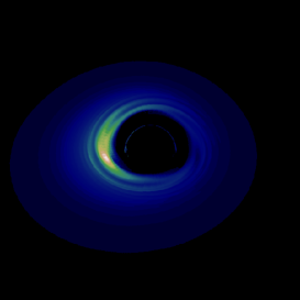
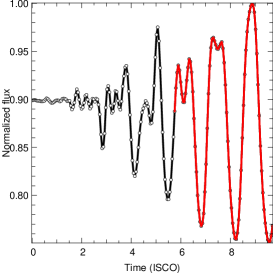
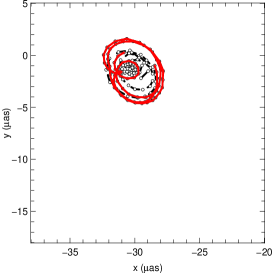
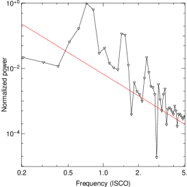
Figure 1: Image (upper left), light curve (upper right), centroid track (lower left) and power spectrum density (lower right) of a two-dimensional disc subject to the RWI, seen under an inclination of $45^{\circ}$. The thick red part of the light curve and centroid track shows 2 h of data, which is the duration we assume for the flare. The red line on the lower right panel shows a power-law spectrum with index $-2.2$, for comparison with Fig. 2.

Fig. 1 shows the image of a two-dimensional disc with the RWI fully developed, seen with an inclination of $45^{\circ}$, together with the simulated light curve, centroid track and power spectrum density. These data last around $10\,T_{\mathrm{ISCO}}$ which translates to around $5$ h for a $4.31\,10^{6}\,M_{\odot}$ Schwarzschild black hole. The details of the RWI modulation will depend on the flare’s parameters. Assuming that the flare can be observed for around $2$ h only and that the small-scale modulation is strong, we select the last $2$ h of our simulated data (in red color in Fig. 1), corresponding to the maximum modulation of the light curve. This choice is not very important as what matters most is the Gaussian modulation that dictates the level of astrometric noise. In the power spectrum density (right panel of Fig. 1), the modal signature of the RWI appears clearly with peaks at once, twice and three times a fundamental frequency which is a bit less than the ISCO frequency (as the instability is triggered at a radius close but larger than the ISCO radius).

The red-color part of the light curve depicted in the upper right panel of Fig. 1 is then modulated by a Gaussian of full width at half maximum adjusted in order to get a factor-two increase of the light curve. The final light curve of the RWI flare model is illustrated in the left panel of Fig. 4.

2.3 Red noise

Light curves of accretion discs subject to the magnetorotational instability (MRI) leading to red-noise fluctuations were simulated by Armitage & Reynolds (2003). These authors performed magnetohydrodynamical (MHD) simulations of an accretion disc surrounding a Schwarzschild black hole, described by a Paczyńsky & Wiita (1980) pseudo-newtonian potential. The vertically averaged magnetic stress is used as a proxy for the dissipation, and light curves can be readily simulated from the MHD data.

Here we use the same MHD data and follow Armitage & Reynolds (2003) to express the emitted intensity integrated over a range of infrared frequencies:

$$I^{\mathrm{em}}_{\mathrm{IR}}\propto\frac{B_{r}B_{\varphi}\left(r,\varphi,t\right)}{\langle B_{r}B_{\varphi}\rangle\left(r\right)}F_{\mathrm{PT}}\left(r\right)$$ (3)

where the $B_{r}B_{\varphi}$ terms are vertically integrated magnetic field components and the average of the denominator is done over azimuthal direction $\varphi$ and time $t$. The $F_{\mathrm{PT}}(r)$ term is the standard expression of a two-dimensional disc’s flux from Page & Thorne (1974).

We refer to the original work by Armitage & Reynolds (2003) for more details on the numerical MHD simulations. Let us note that this work was developed for relatively geometrically thin accretion disc. We use these results for the geometrically thick Sgr A* accretion flow assuming that the details of the vertical structure of the flow does not impact our results. As the astrometric data we model are only sensitive to the displacement of the centroid projected on the observer’s sky, we believe this is a sound assumption. Likewise, the heuristic emission law that we consider (Eq. 3) fits our goal of developing a first-order, simple red-noise model. We do not claim that such a model is realistic enough to test the details of a red-noise varying accretion structure surrounding Sgr A*, but this is not (yet) our goal. We have checked that considering a different emission law than the Page-Thorne prescription does not change noticeably the centroid position.

We note that more realistic models of the accretion flow surrounding Sgr A* have been extensively developed in the past few years (e.g. Goldston et al., 2005; Noble et al., 2007; Chan et al., 2009; Mościbrodzka et al., 2009; Dexter et al., 2010; Shcherbakov et al., 2012). We will devote future work to developing our model in this way in order to become able to study in detail the photometric, spectroscopic and polarimetric signatures of a red-noise accretion flow surrounding Sgr A*.

Fig. 2 shows an image of the red-noise model, the long-term light curve, the associated centroid track and the power spectrum density for an inclination of $45^{\circ}$. The power spectrum density shows a clear red-noise profile. The increase (during $\approx 40\,T_{\mathrm{ISCO}}$) and subsequent decrease of the light curve are due to variations of the accretion rate that are related to the simulation’s initial conditions. These long-term variations would not show in real data (see more details in Armitage & Reynolds, 2003).

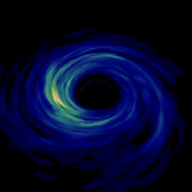
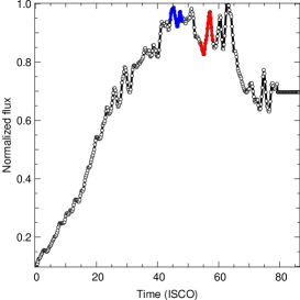
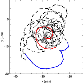
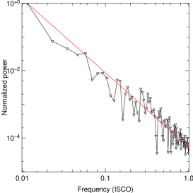
Figure 2: Image (upper left), light curve (upper right), centroid track (lower left) and power spectrum density (lower right) of a two-dimensional disc subject to red-noise fluctuations, seen under an inclination of $45^{\circ}$. Two $2$ h-long parts of the simulated data that are used for the GRAVITY simulations are shown in red and blue in the light curve and centroid track. The blue data correspond to a length of centroid track close to maximum while the red data correspond to a length close to minimum. The red line in the lower right panel shows a power law $f^{-2.2}$.

As we are interested in only a few ISCO periods of data, we only consider the part of the light curve where the long-term fluctuation of the accretion rate is least visible, i.e. between $\approx 40\,T_{\mathrm{ISCO}}$ and $\approx 60\,T_{\mathrm{ISCO}}$. In this range, we have selected two light curves of $2$ h, corresponding to two extreme extensions of the centroid track of the source: one little extended track (red in Fig. 2) and one more extended track (blue). These two extreme cases show that the extension of the centroid track can vary by a factor of $2$ depending on the initial conditions of the red-noise model. In order to take this into account, $50\%$ of the simulated astrometric data will use the little extended track case, and $50\%$ the more extended case.

The central panel of Fig. 4 shows the Gaussian-modulated red-noise light curve that will be used in the following. This light curve corresponds to the extended track of the source (blue data in Fig. 2).

2.4 Ejected blob model

We have developed MHD simulations of a blob of electrons ejected along the $z$ axis (orthogonal to the equatorial plane) from an initial altitude of $z_{\mathrm{ej}}=6\,r_{g}$ along the $z$ axis, where $r_{g}=GM/c^{2}$. The MHD simulation is performed using the AMRVAC code (Keppens et al., 2011). The simulations are done in two dimensions in the plane $(x,z)$ where $x$ is a coordinate in the equatorial plane. The blob is then made three-dimensional by assuming it is axisymmetric. The simulations are done using a pseudo-Newtonian potential. The grid size is of around $0.1~{}r_{g}$. The magnetic field is assumed to remain constant, with a norm of $20$ G (see e.g. Liu et al., 2004) and vertical field lines orthogonal to the equatorial plane. This is a very simplifying assumption, but here as well as in the other models, we are not (yet) interested in studying the details of an ejected blob. Our goal is to determine the astrometric signature of a single blob of plasma (not a continuous jet) when ejected linearly from the vicinity of Sgr A*. The density is computed as a function of time and the blob is defined as the region where density is higher than $80\%$ of its maximum value. The typical radius of the initial blob is $R\approx 3\,r_{g}$. The main parameter of the model is the ejection velocity that we choose equal to $v_{\mathrm{ej}}=0.4\,c$ which is approximately equal to the Keplerian orbital velocity at ISCO. For such an ejection velocity, the blob is not able to escape the black hole attraction and ultimately falls back onto it (the escape speed for the blob we model, with an initial altitude of $z_{\mathrm{ej}}=6\,r_{g}$, is of around $0.45\,c$). This choice of ejection velocity is dictated by the fact that the flare is assumed to last around $4$ ISCO periods. With our choice of ejection velocity, the complete simulation, from the blob ejection to its coming back to the same location ($z=6\,r_{\mathrm{g}}$, the bottom of the simulation box), lasts around $5$ ISCO periods. For higher velocities, the blob escapes too fast to be seen for $\approx 2~{}$h. Moreover, the observed centroid track will become longer than the sub-millimeter constraint on Sgr A* wandering (Reid et al., 2008). As the plasmon model leads to sub-millimeter emission following infrared emission, the infrared position wander should stay below the boundary of Reid et al. (2008). For smaller velocities, the blob falls back onto the black hole too fast as well. Thus our choice of velocity is well adapted for a long-duration flare. The velocity is oriented along the $z$ axis and the blob is thus assumed to be ejected orthogonally to the equatorial plane in the $z>0$ direction. As the simulation box takes only into account the $z>6\,r_{g}$ region, the interaction between the falling blob and the accretion disc is not modelled. However, the rapidly decreasing blob’s density will be much smaller than the disc’s density at the impact, and its temperature will as well be much smaller. It is thus unlikely that the interaction of the falling blob with the disc would lead to any observable effect.

The blob is assumed to be emitting synchrotron infrared radiation. Following the literature to compute this emission (see for instance Falcke & Biermann, 1995), we express the emission and absorption coefficients according to (Rybicki & Lightman, 1986)

$$j_{\nu}^{\mathrm{blob}} = C\,2\pi^{3/2}\frac{\sqrt{3}q^{3}B}{4\pi mc^{2}(p+1)}\Gamma\left(\frac{p}{4}+\frac{19}{12}\right)$$

$$\Gamma\left(\frac{p}{4}-\frac{1}{12}\right)\frac{\Gamma\left(\frac{7}{4}-\frac{p}{4}\right)}{\Gamma\left(\frac{9}{4}-\frac{p}{4}\right)}\left(\frac{2\pi mc\nu}{3qB}\right)^{-(p-1)/2}$$

and

$$\alpha_{\nu}^{\mathrm{blob}} = C\,2\pi^{3/2}\frac{\sqrt{3}q^{3}}{8\pi m}\left(\frac{3q}{2\pi m^{3}c^{5}}\right)^{p/2}B^{(p+2)/2}$$

$$\Gamma\left(\frac{3p+2}{12}\right)\Gamma\left(\frac{3p+22}{12}\right)\frac{\Gamma\left(\frac{5+p}{4}\right)}{\Gamma\left(\frac{7+p}{4}\right)}\nu^{-(p+4)/2}$$

where $B$ is the magnetic field, $C$ and $p$ are defined by assuming that the electrons energy density is a power law, $n(E)=C\,E^{-p}$, where $E$ is the energy, $q$ and $m$ are the electron’s charge and mass. The gamma function $\Gamma$ is used. Here the pitch angle between the magnetic field and the electron velocity has been averaged, as the electrons have a vertical bulk motion, but have random-oriented velocity in the blob’s frame. Let us note that this random velocity is much bigger than the bulk velocity. Electrons have indeed Lorentz factors of at least $\gamma\approx 100$ while the ejection velocity of $0.4\,c$ corresponds to $\gamma_{\mathrm{ej}}\approx 1$.

Assuming equipartition between the magnetic and electrons energy densities,

$$\frac{B^{2}}{8\pi}=C\int_{\gamma_{m}}^{\gamma_{M}}\gamma mc^{2}\gamma^{-p}\mathrm{d}\gamma$$ (6)

where $\gamma$ is the Lorentz factor and $\gamma_{m}$ and $\gamma_{M}$ are the minimal and maximal Lorentz factors of the electrons. This immediately gives

$$C=\frac{B^{2}}{8\pi mc^{2}}\frac{2-p}{\gamma_{M}^{2-p}-\gamma_{m}^{2-p}}$$ (7)

for $p\neq 2$. In the following, we assume $p=4$, $\gamma_{m}=100$ and $\gamma_{M}=100\,\gamma_{m}$.

The radiative transfer equation can thus be straightforwardly integrated in the blob, which is done by the GYOTO code. As only the bulk velocity of the blob is known, and not the instantaneous random velocity of the emitting electrons, it is not possible to compute the redshift factor $g$ related to the emitter’s 4-velocity, such that the observed and emitted specific intensities are related by $I_{\nu}^{\mathrm{obs}}=g^{4}I_{\nu}^{\mathrm{em}}$. This factor is thus imposed to be constant for all GYOTO screen pixels. This boils down to assuming that the emitter is on averaged at rest in the blob’s frame, which is true as in this frame the emitter’s velocity has random orientation.

Fig. 3 shows a ray-traced image, the light curve and the centroid path of the blob model as seen from an inclination of $45^{\circ}$. The variation of the light curve is mainly due to the change of projected area of the blob. It first expands, reaches a maximum, and is then divided into two sub-blobs due to tidal effects, that fall back onto the black hole. Let us note that the total angular displacement of the blob on the observer’s sky is of around $100~{}\mu$as in approximately $2$ h. Such a displacement is of the same order as the detected level of Sgr A* wandering by sub-millimeter interferometry (Reid et al., 2008). Higher ejection velocities would lead to exceeding this limit.

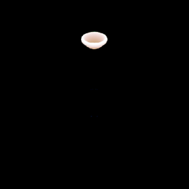
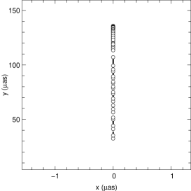
Figure 3: Image (left), light curve (centre) and centroid track (right) of the ejected blob, seen under an inclination of $45^{\circ}$. In the left panel, the blob is close to its maximal altitude, before falling down onto the black hole. Its typical radius at this moment is of around $4~{}r_{g}$.

Fig. 4 shows the three light curves for all flare models, at $45^{\circ}$ of inclination, that will be used to generate GRAVITY simulations. The light curves look different from one model to the other: it may seem likely that models could be distinguished only by studying the observed flux. However, as stated above, our RWI and RN models are restricted to model the small-scale variation of the flux and are not meant to reproduce all aspects of observed light curves. As a consequence, our simulated light curves should not be compared to observed data. Their only goal in this article is to give a realistic evolution of the K-band magnitude of the source, and thus of the GRAVITY astrometric error.

Next Section describes the GRAVITY data acquisition.

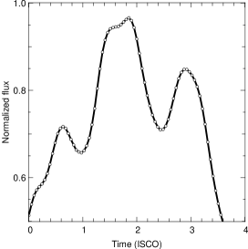
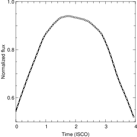
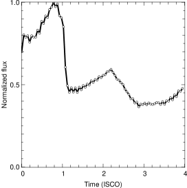
Figure 4: Light curves of the three models investigated, as used for the GRAVITY simulations: RWI (left), red noise (centre), blob (right). The RWI and RN light curves from Figs. 1 and 2 are here modulated by a Gaussian. The time is given in units of the ISCO period, which is $\approx 30$ min for a Schwarzschild black hole of $4.31\,10^{6}\,M_{\odot}$. These three light curves look quite different, but observed infrared data show a large variety (see e.g. Do et al., 2009; Hamaus et al., 2009).

3 Simulation of a GRAVITY observation

3.1 Simulating GRAVITY astrometric data

The simulation of GRAVITY astrometric data given some model of emission in the vicinity of Sgr A* is described in detail in Vincent et al. (2011). We will only briefly summarize the main steps here for convenience.

The light curve and centroid track of some model being known, a set of angular positions on sky and intensities $(x_{\mathrm{th}}(t),y_{\mathrm{th}}(t),I_{\mathrm{th}}(t))$ are available for all observing times $t$. Here the subscript indicates that these quantities are theoretical, computed by our set of numerical codes described above. The $y$ coordinate is along the normal to the equatorial plane, while $x$ is orthogonal to $y$.

From this, a set of theoretical complex visibilities

$$V_{\mathrm{th}}\left(t,u,v\right)=I_{\mathrm{th}}(t)\,e^{-2\,i\,\pi\,\left(u\,x_{\mathrm{th}}(t)+v\,y_{\mathrm{th}}(t)\right)}$$ (8)

can be computed for all spatial frequencies $(u,v)$. Given that GRAVITY uses four telescopes (i.e. six baselines) and five spectral channels in its most sensitive mode, there are $30$ pairs of $(u,v)$ points and hence $30$ values of theoretical complex visibilities associated to one given set $(x_{\mathrm{th}}(t),y_{\mathrm{th}}(t),I_{\mathrm{th}}(t))$.

Realistic noise is added to these theoretical visibilities (see the detailed description of the sources of noise in Vincent et al., 2011, and the short presentation of detection noise in the Appendix) in order to get the simulated observed visibilities $V_{\mathrm{obs}}\left(t,u,v\right)$.

The retrieved astrometric data $(x_{\mathrm{obs}}(t),y_{\mathrm{obs}}(t))$ are then found by fitting the observed visibilities, assuming intensity can be measured with $10\%$ accuracy, which is the typical photometric accuracy of GRAVITY. The fitting procedure is done using the Levenberg-Marquardt algorithm as implemented in the Yorick language by the lmfit routine. The astrometric error on this retrieved position is found as a function of the source magnitude at time $t$ by using the GRAVITY astrometric error study presented in Vincent et al. (2011). As the orientation of the normal to the black hole’s equatorial plane with respect to the axes of the instrument’s point spread function (PSF) is not known, we assume an equal astrometric error in the two orthogonal direction $x$ and $y$ (that is to say, we assume that the normal to the equatorial plane makes an angle of $45^{\circ}$ with respect to the PSF axes).

3.2 Simulating a flare observation by GRAVITY

We consider one night of observation chosen on 2014 April 15. Choosing the $15^{\mathrm{th}}$ day of the month is purely arbitrary. However, the choice of the month has an impact on the total time during which the GC is observable. On 2014 April 15, the GC is observable for a little more than 5 hours (as a comparison, it would be observable for 9 hours in June). As the duration of a flare is assumed to be $2$ h, it is possible to observe the whole event.

The integration time of the instrument is set to $100$ s, allowing to follow the dynamics of the flare. The Earth rotation during one elementary block is supposed to be negligible because the trace in the $(u,v)$ plane during one integration block is perfectly linear and can be replaced by its average.

The light curve is scaled by the brightest magnitude of the flare, which is chosen to be $m_{\mathrm{K}}=14$ or $m_{\mathrm{K}}=15$. The brightest magnitude is still a realistic choice for a brigth flare, as the most powerfull such event has been observed at $m_{\mathrm{K}}=13.5$ (Dodds-Eden et al., 2011).

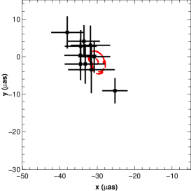
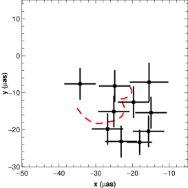
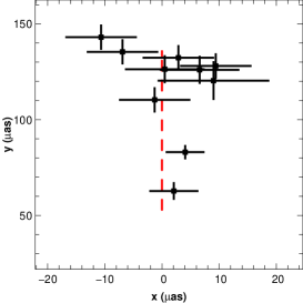
Figure 5: GRAVITY observation simulation of one night with a flare due to the RWI model (left), the red-noise model (centre) or the blob model (right), with inclination $45^{\circ}$. The dashed red line is the theoretical centroid track. The error bars take into account the realistic astrometric performances of the instrument. The axes are graduated in microarcseconds. Mind the different vertical scaling of the panels.

Fig. 5 shows a simulation of one such night of observation by GRAVITY for all flare models considered here, the inclination being assumed to be $45^{\circ}$. The size of the error bars are not all the same as they depend on the magnitude of the flare at the time of observation. If the brightest magnitude is $m_{\mathrm{K}}=14$, it will decrease to reach at the lowest level $m_{\mathrm{K}}=14.75$, which translates to a precision for a single observation (no averaging) of respectively $8~{}\mu$as and $16~{}\mu$as (Vincent et al., 2011). The retrieved data are averaged in order to get a better precision and only $10$ astrometric data points are conserved from the initial $\approx 70$ retrieved data points, hence a factor $\approx 2.5$ better in precision. This is the reason why the error bars are better than the single-observation precision.

4 Distinguishing an ejected blob from GRAVITY astrometric data

4.1 Directional dispersion

In this Section we investigate whether the different flare models can be distinguished by computing the dispersion of the GRAVITY retrieved positions. The directional dispersions $\sigma_{x}$ and $\sigma_{y}$ are defined as:

$$\sigma_{x} = \sqrt{\frac{1}{N-1}\sum\left(x-x_{\mathrm{moy}}\right)^{2}},$$ (9)

$$\sigma_{y} = \sqrt{\frac{1}{N-1}\sum\left(y-y_{\mathrm{moy}}\right)^{2}},$$

where $N$ is the number of averaged data, $x_{\mathrm{moy}}$ and $y_{\mathrm{moy}}$ are the averaged of the $x$ and $y$ retrieved coordinates. One value of directional dispersion $(\sigma_{x}$, $\sigma_{y})$ is computed for every simulated night of observation. In the framework of a Monte Carlo analysis, we simulate $1000$ nights of observation for all three models. The histograms of the resulting dispersions are analysed in the following Section.

4.2 Results

Figs. 6 and 7 show the histograms of directional dispersion of the RWI, RN and blob models when the inclination and brightest magnitude of the flare are varied in $i\in[5^{\circ};45^{\circ};85^{\circ}]$ and $m_{\mathrm{K}}\in[14;15]$.

The RWI and RN are not distinguishable, even if many bright $(m_{\mathrm{K}}=14)$ and long ($2$ h) flares were observed, as their respective histograms are nearly superimposed. This holds whatever the inclination. However, the blob model histograms are very clearly separated from the two other models at medium and high inclination, both for a brightest flare magnitude of $m_{\mathrm{K}}=14$ and $m_{\mathrm{K}}=15$. At small inclination ($i\approx 5^{\circ}$), all models are indistinguishable.

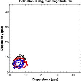
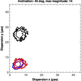
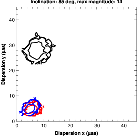
Figure 6: Histograms of directional dispersions $(\sigma_{x},\sigma_{y})$ (defined in Eq. 9) of the GRAVITY astrometric data retrieved in the framework of the RWI (blue), RN (red) and blob (black) models. The inclination is $5^{\circ}$ (left), $45^{\circ}$ (centre) or $85^{\circ}$ (right). The brightest magnitude of the flare is always $m_{\mathrm{K}}=14$. The contours encompass respectively around $68\%$, $95\%$ and $99\%$ of the simulated $1000$ nights.The blob model is easily distinguished from the two other models at medium and high inclination.

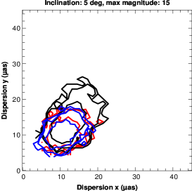
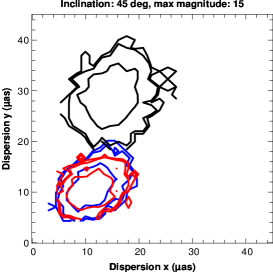
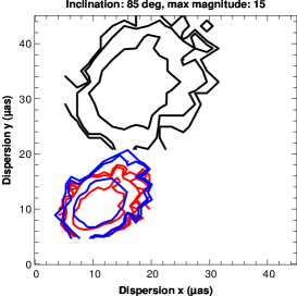
Figure 7: Same as Fig. 6 with $m_{\mathrm{K}}=15$. The blob model is still easily distinguished from the two other models at medium and high inclination.

It is interesting to determine whether the distinction between the blob models and its alternatives is strongly dependent on the flare duration. Fig. 8 shows the directional dispersion obtained when the flare duration is reduced from $2$ h to $1$ h $30$, for a brightest magnitude of $m_{\mathrm{K}}=15$. It shows that the blob model can still be easily distinguished. In order to model a shorter flare in the framework of the blob model, the ejection velocity has been reduced from $0.4~{}c$ to $0.36~{}c$, leading to a smaller maximum altitude of the blob ($60~{}\mu$as as compared to $100~{}\mu$as, at $45^{\circ}$ of inclination). When reducing the flare duration (and hence the blob ejection velocity) to approximately $1$ h, it becomes very difficult to distinguish the models. In this case, the blob’s motion has a vertical extension of around $20~{}\mu$as, which gets very close to the typical extension of the centroid motion for RWI and RN models. Fig. 9 shows that even for a brightest magnitude of $m_{\mathrm{K}}=14$ and an inclination of $85^{\circ}$, the directional dispersion of the three models overlap. However, the distinction is still marginally possible in this case, but many events would be necessary to disentangle clearly the models.

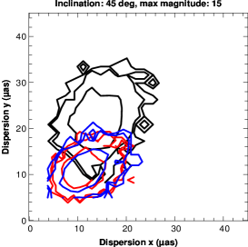
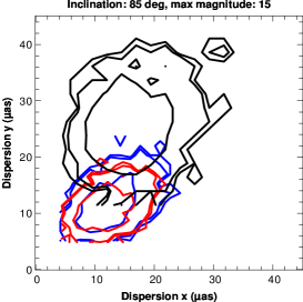
Figure 8: Histograms of the directional dispersion for a shorter flare that lasts approximately $1$ h $30$ (as compared to $2$ h for Fig. 6 - 7), with a brightest magnitude of $m_{\mathrm{K}}=15$ and an inclination of $45^{\circ}$ (left) or $85^{\circ}$ (right). The distinction of the blob model is still possible.

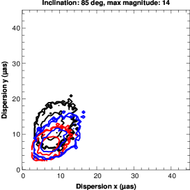
Figure 9: Histograms of the directional dispersion for an even shorter flare that lasts approximately $1$ h (as compared to $2$ h for Figs. 6 - 7), with a brightest magnitude of $m_{\mathrm{K}}=14$ and an inclination of $85^{\circ}$. The distinction of the blob model is still marginally possible.

5 Conclusion

We have analysed the ability of the near-future GRAVITY instrument to distinguish different flare models, depending only on their astrometric signatures. We show that the ejection of a blob can be distinguished from alternative models provided the ejection direction is not face-on for the observer. This result holds for a reasonably long flare ($\gtrsim 1$ h $30$) with a brightest magnitude in K-band of $14\lesssim m_{\mathrm{K}}\lesssim 15$.

Our models are very simple for the time being. In particular, we use a geometrically thin disk approximation with very simple emission laws and a pseudo-Newtonian potential for all MHD simulations. However, this simple framework allows to generate images of Sgr A* accretion flow that looks rather similar to more complex simulations.

The main result of our simulations is that GRAVITY will be able to distinguish an ejection model as compared to ”disk-glued” models. This result is rather natural, as most models of disk-like (be it geometrically thin or thick) accretion structures will give rise to typical crescent-shape images (Kamruddin & Dexter, 2013), and will lead to rather similar centroid tracks. We believe that this result is robust and will not be changed by developing more sophisticated simulations.

Our result is important in the sense that it demonstrates the ability of GRAVITY to make an observable difference between categories of flare models, which has not been possible so far with current instrumentation.

Future work will be dedicated to determining to what extent can the astrometric data of GRAVITY help distinguish models of the two first astrometric signature classes, as defined in Section 1 (typically, the red-noise and RWI models). This will demand resorting not only on astrometry but on other signatures as well, such as photometry and polarimetry. Let us repeat here that our current results, allowing to distinguish an ejected blob, only use astrometric data, thus only a part of the total flare data.

Future work will also be dedicated to modelling various flare models using GRMHD simulations in order to be able to study the impact of the spin parameter on the observables. Such a study of Sgr A* variability in GRMHD simulations is currently developed by various groups (see e.g. Dexter et al., 2009; Dolence et al., 2012; Henisey et al., 2012; Dexter & Fragile, 2013; Shcherbakov & McKinney, 2013).

Appendix A Detection noise for GRAVITY observation

For completeness we discuss here the sources of detection noise that will affect GRAVITY observations. This discussion comes from Vincent et al. (2011).

GRAVITY will use the four Very Large Telescope Unit Telescopes (UT) to observe Sgr A*. Each baseline will combine the beams of intensities $I_{p}$ and $I_{q}$ delivered by two telescopes labelled $p$ and $q$. Let the intrinsic visibility modulus and phase of the observed object be $V_{\mathrm{obj}}$ and $\phi_{\mathrm{obj}}$. Let $\delta\phi$ be the phase shift between the two channels from telescope $p$ and $q$. The short-exposure noiseless combined intensity is:

$$I(\delta\phi)=I_{p}+I_{q}+2\sqrt{I_{p}I_{q}}V_{\mathrm{obj}}\mathrm{cos}(\delta\phi+\phi_{\mathrm{obj}}+\phi_{\mathrm{piston,short}})$$ (10)

where $\phi_{\mathrm{piston,short}}$ is the short-exposure piston phase.

It is sufficient to get four samples of this function in order to retrieve the visibility modulus and the phase of the object. Indeed, if the four following quantities are computed:

$$A = I(0),$$ (11)

$$B = I(\frac{\pi}{2}),$$

$$C = I(\pi),$$

$$D = I(\frac{3\,\pi}{2}),$$

then it is easy to show that the complex visibility of the object is given by:

$$V_{\mathrm{obj}}e^{i\,\phi_{\mathrm{obj}}}=2\frac{(A-C)-i\,(B-D)}{A+B+C+D}.$$ (12)

In order to be able to simulate realistic quantities, we now take into account the various sources of noises affecting the different quantities that have been introduced.

Let $N_{\rm{ph}}$ be the number of photons arriving from each of the $N_{\rm{tel}}$ telescopes of the interferometer. Each set of $N_{\rm{ph}}$ photons will be dispatched to the $N_{\rm{tel}}-1$ other telescopes. Then $\frac{2N_{\rm{ph}}}{N_{\rm{tel}}-1}$ photons will be present in the baseline between two telescopes. Let $T$ be the transmission of the instrument multiplied by the quantum yield, estimated to be 0.009. The mean number of photo-electrons $\langle m\rangle$ per sample per baseline is:

$$\langle m\rangle=\frac{2N_{\rm{ph}}T}{4(N_{\rm{tel}}-1)}.$$ (13)

Hence the shot noise: $\sigma_{\mathrm{shot}}=\sqrt{\langle m\rangle}$. It is assumed that the number of read out noise electrons is equal to $\sigma_{\mathrm{RON}}^{2}=36$. Given the rate of dark current electrons $N_{\mathrm{dark}}=100\;\rm{s}^{-1}$, the variance of the detection noise per integration time $\tau$ is:

$$\sigma^{2}_{\mathrm{detec}}=\sigma_{\mathrm{shot}}^{2}+\sigma_{\mathrm{RON}}^{2}+N_{\mathrm{dark}}\,\tau.$$ (14)

Taking this noise into account, and assuming a gaussian distribution for the various noise contributions, it is possible to compute a realization of the detection noise $n_{A},n_{B},n_{C},n_{D}$ corrupting the four A,B,C,D signals, hence the noise on the object complex visibility.

References

- Armitage & Reynolds (2003) Armitage P. J., Reynolds C. S., 2003, \mnras, 341, 1041
- Baganoff et al. (2001) Baganoff F. K., Bautz M. W., Brandt W. N., Chartas G., Feigelson E. D., Garmire G. P., Maeda Y., Morris M., Ricker G. R., Townsley L. K., Walter F., 2001, \nat, 413, 45
- Bardeen (1973) Bardeen J. M., 1973, in Dewitt C., Dewitt B. S., eds, Black Holes (Les Astres Occlus) Timelike and null geodesics in the Kerr metric.. pp 215–239
- Chan et al. (2009) Chan C.-k., Liu S., Fryer C. L., Psaltis D., Özel F., Rockefeller G., Melia F., 2009, ApJ, 701, 521
- Clénet et al. (2005) Clénet Y., Rouan D., Gratadour D., Marco O., Léna P., Ageorges N., Gendron E., 2005, \aap, 439, L9
- Dexter et al. (2009) Dexter J., Agol E., Fragile P. C., 2009, ApJL, 703, L142
- Dexter et al. (2010) Dexter J., Agol E., Fragile P. C., McKinney J. C., 2010, ApJ, 717, 1092
- Dexter et al. (2012) Dexter J., Agol E., Fragile P. C., McKinney J. C., 2012, Journal of Physics Conference Series, 372, 012023
- Dexter & Fragile (2013) Dexter J., Fragile P. C., 2013, MNRAS, 432, 2252
- Do et al. (2009) Do T., Ghez A. M., Morris M. R., Yelda S., Meyer L., Lu J. R., Hornstein S. D., Matthews K., 2009, \apj, 691, 1021
- Dodds-Eden et al. (2011) Dodds-Eden K., Gillessen S., Fritz T. K., Eisenhauer F., Trippe S., Genzel R., Ott T., Bark H., Pfuhl O., Bower G., Goldwurm A., Porquet D., Trap G., Yusef-Zadeh F., 2011, \apj, 728, 37
- Dodds-Eden et al. (2010) Dodds-Eden K., Sharma P., Quataert E., Genzel R., Gillessen S., Eisenhauer F., Porquet D., 2010, \apj, 725, 450
- Dolence et al. (2012) Dolence J. C., Gammie C. F., Shiokawa H., Noble S. C., 2012, \apjl, 746, L10
- Eckart et al. (2009) Eckart A., Baganoff F. K., Morris M. R., Kunneriath D., Zamaninasab M., Witzel G., Schödel R., García-Marín M., et al. 2009, \aap, 500, 935
- Eckart et al. (2008) Eckart A., Schödel R., García-Marín M., Witzel G., Weiss A., Baganoff F. K., Morris M. R., Bertram T., et al. 2008, \aap, 492, 337
- Eisenhauer et al. (2011) Eisenhauer F., Perrin G., Brandner W., Straubmeier C., Perraut K., Amorim A., Schöller M., Gillessen S., et al. 2011, The Messenger, 143, 16
- Falanga et al. (2007) Falanga M., Melia F., Tagger M., Goldwurm A., Bélanger G., 2007, \apjl, 662, L15
- Falcke & Biermann (1995) Falcke H., Biermann P. L., 1995, \aap, 293, 665
- Falcke et al. (2000) Falcke H., Melia F., Agol E., 2000, ApJL, 528, L13
- Genzel et al. (2003) Genzel R., Schödel R., Ott T., Eckart A., Alexander T., Lacombe F., Rouan D., Aschenbach B., 2003, \nat, 425, 934
- Ghez et al. (2008) Ghez A. M., Salim S., Weinberg N. N., Lu J. R., Do T., Dunn J. K., Matthews K., Morris M. R., Yelda S., Becklin E. E., Kremenek T., Milosavljevic M., Naiman J., 2008, \apj, 689, 1044
- Ghez et al. (2004) Ghez A. M., Wright S. A., Matthews K., Thompson D., Le Mignant D., Tanner A., Hornstein S. D., Morris M., Becklin E. E., Soifer B. T., 2004, \apjl, 601, L159
- Gillessen et al. (2009) Gillessen S., Eisenhauer F., Trippe S., Alexander T., Genzel R., Martins F., Ott T., 2009, \apj, 692, 1075
- Goldston et al. (2005) Goldston J. E., Quataert E., Igumenshchev I. V., 2005, ApJ, 621, 785
- Hamaus et al. (2009) Hamaus N., Paumard T., Müller T., Gillessen S., Eisenhauer F., Trippe S., Genzel R., 2009, \apj, 692, 902
- Henisey et al. (2012) Henisey K. B., Blaes O. M., Fragile P. C., 2012, \apj, 761, 18
- Kamruddin & Dexter (2013) Kamruddin A. B., Dexter J., 2013, MNRAS, 434, 765
- Keppens et al. (2011) Keppens R., Meliani Z., van Marle A., Delmont P., Vlasis A., van der Holst B., 2011, Journal of Computational Physics, doi:10.1016/j.jcp.2011.01.020,
- Liu et al. (2004) Liu S., Petrosian V., Melia F., 2004, ApJL, 611, L101
- Markoff et al. (2001) Markoff S., Falcke H., Yuan F., Biermann P. L., 2001, \aap, 379, L13
- Mościbrodzka et al. (2009) Mościbrodzka M., Gammie C. F., Dolence J. C., Shiokawa H., Leung P. K., 2009, ApJ, 706, 497
- Noble et al. (2007) Noble S. C., Leung P. K., Gammie C. F., Book L. G., 2007, Classical and Quantum Gravity, 24, 259
- Paczyńsky & Wiita (1980) Paczyńsky B., Wiita P. J., 1980, \aap, 88, 23
- Page & Thorne (1974) Page D. N., Thorne K. S., 1974, \apj, 191, 499
- Reid et al. (2008) Reid M. J., Broderick A. E., Loeb A., Honma M., Brunthaler A., 2008, \apj, 682, 1041
- Rybicki & Lightman (1986) Rybicki G. B., Lightman A. P., 1986, Radiative Processes in Astrophysics. Wiley-VCH , June 1986
- Shcherbakov & McKinney (2013) Shcherbakov R. V., McKinney J. C., 2013, ApJL, 774, L22
- Shcherbakov et al. (2012) Shcherbakov R. V., Penna R. F., McKinney J. C., 2012, ApJ, 755, 133
- Tagger & Melia (2006) Tagger M., Melia F., 2006, \apjl, 636, L33
- Tagger & Varnière (2006) Tagger M., Varnière P., 2006, \apj, 652, 1457
- Vincent et al. (2013) Vincent F. H., Meheut H., Varniere P., Paumard T., 2013, \aap, 551, A54
- Vincent et al. (2011) Vincent F. H., Paumard T., Gourgoulhon E., Perrin G., 2011, Classical and Quantum Gravity, 28, 225011
- Vincent et al. (2011) Vincent F. H., Paumard T., Perrin G., Mugnier L., Eisenhauer F., Gillessen S., 2011, \mnras, 412, 2653
- Yusef-Zadeh et al. (2006) Yusef-Zadeh F., Bushouse H., Dowell C. D., Wardle M., Roberts D., Heinke C., Bower G. C., Vila-Vilaró B., Shapiro S., Goldwurm A., Bélanger G., 2006, \apj, 644, 198
- Yusef-Zadeh et al. (2006) Yusef-Zadeh F., Roberts D., Wardle M., Heinke C. O., Bower G. C., 2006, \apj, 650, 189
- Zamaninasab et al. (2011) Zamaninasab M., Eckart A., Dovčiak M., Karas V., Schödel R., Witzel G., Sabha N., García-Marín M., Kunneriath D., Mužić K., Straubmeier C., Valencia-S M., Zensus J. A., 2011, \mnras, 413, 322