Irreversible processes without energy dissipation in an isolated Lipkin-Meshkov-Glick model

Abstract

For a certain class of isolated quantum systems, we report the existence of irreversible processes in which the energy is not dissipated. After a closed cycle in which the initial energy distribution is fully recovered, the expectation value of a symmetry-breaking observable changes from a value different from zero in the initial state, to zero in the final state. This entails the unavoidable loss of a certain amount of information, and constitutes a source of irreversibility. We show that the von Neumann entropy of time-averaged equilibrium states increases in the same magnitude as a consequence of the process. We support this result by means of numerical calculations in an experimentally feasible system, the Lipkin-Meshkov-Glick model.

I Introduction

A fundamental explanation of entropy production, irreversibility and dissipation is the cornerstone of non-equilibrium statistical mechanics. It is now well known that microscopic time reversibility entails a number of relations between dissipation in any time-dependent process and the thermodynamic properties of the equilibrium initial and final states Jarzynski:11 . For isolated systems, the work dissipated in a cyclic process is linked to the increase of entropy after the forward part, if the system equilibrates to a microcanonical state after each time-dependent process Talkner:08 . But it is also stated that there is a strong connection between irreversibility and information gained or lost by the system, manifested in the physical consequences of the Szilard engine Szilard:29 , and expressed in the Landauer principle of information erasure Landauer:61 . So, a complete description of the entropy production following a thermodynamic transformation requires the account of the information flow Sagawa:10 , and the addition of information reservoirs, besides the traditional heat and chemical baths Jordan:14 .

This is specially relevant in isolated quantum systems that equilibrate to complex equilibrium states Polkovnikov:11 which store relevant information in sets of commuting constants of motion Rigol:07 , or in the coherences between different subspaces of the system in the case of degenerate spectra Puebla:13 ; epl . This means that the Hamiltonian $H$ and the number of particles $N$ are not enough to characterize the equilibrium states and the thermodynamic processes in this kind of systems. Hence, a number of fundamental questions naturally arise. How the extra information stored in the equilibrium state of the system is eroded by an irreversible time-dependent protocol? Must it be explicitly included in the formulation of the Second Law?

In the present article we deal with these questions in a certain class of isolated quantum systems. We report the existence of processes for which the energy is not dissipated, but they are irreversible due to an unavoidable loss of information about the initial symmetry-breaking. Hence, we conclude that this information has to be accounted for a precise definition of irreversibility and for a consistent formulation of the Second Law.

This phenomenon can be observed in systems that exhibit a transition from a normal or non-degenerate, to a double-degenerate phase in the energy spectrum. These systems have an extra discrete symmetry $S$ which labels all the eigenstates, although symmetry-breaking eigenstates can also exist in the double-degenerate phase. After a thermodynamic transformation leading the system from the double-degenerate to the normal region, phase mixing between different symmetry sectors  forces the evolved state to be in a superposition of the different branches of symmetry-breaking. As a consequence, the expectation values of symmetry-breaking observables become zero at the end of the protocol, independently on the initial condition; we can thus conclude that the information about the initial symmetry-breaking is lost at the end of the protocol. On the contrary, observables that are not linked to symmetry-breaking, such as the energy, are not affected; if the protocol is slow enough, the energy distribution is exactly recovered at the end. So, an unexpected kind of irreversibility arises, not related to energy dissipation, but to the loss of significant information about the initial state. We support our conclusions with numerical calculations in an experimentally feasible system Zibold:10 ; Gross:10 .

The paper is organized as follows. In Sec. II we describe the model and the protocol used to implement the irreversible processes. In Sec. III we present the main numerical results. In Sec. IV we provide an interpretation in terms of the von Neumann entropy. In Sec. V we propose a mechanism which accounts for this unexpected irreversible behavior. Finally, in Sec. VI we summarize the main conclusions.

II Model and protocol

II.1 Many-body quantum system

We illustrate this phenomenon in the Lipkin-Meshkov-Glick model Lipkin:65 ; Vidal:04 that describes $N$ interacting particles of $\frac{1}{2}$-spin coupled to an external field, which has been experimentally explored with a great level of control, accuracy and isolation Zibold:10 . In its most general version, it includes both $J_{x}^{2}$ and $J_{y}^{2}$ interaction terms, and two free parameters: one for the coupling strength and another for the deformation Vidal:04 . However, its most recent experimental realization Zibold:10 consists of a condensate of $N$ atoms distributed between two different modes, whose interaction is governed by the $J_{x}^{2}$ term. In this way, the model reduces to the following Hamiltonian

$$H=\chi J_{x}^{2}-\Omega J_{z},$$ (1)

where $\vec{J}$ is the Schwinger pseudospin representation of the $N$ two-level atom system; the parameters $\chi$ and $\Omega$ describe the nonlinearity of the atom-atom interaction and the linear coupling strength, respectively Zibold:10 ; $J_{x}$ gives the difference of population between the two modes, and $J_{y}$ and $J_{z}$ the corresponding coherences. Since $J^{2}$ is a conserved quantity, we consider only the sector of maximum angular momentum, i.e. $J=N/2$. This is precisely what has been measured in recent experiments Zibold:10 ; Gross:10 . The rest of sectors behave in the same qualitative way; all are equivalent to the one with $J=N/2$, but with different effective number of particles and very large degeneracies, due to the many different possibilities of obtaining a certain value of the angular momentum $J<N/2$ by coupling $N$ particles of $\frac{1}{2}$-spin.

The Hamiltonian (1) holds a discrete and global symmetry $S$, which leads to another conserved quantity, the parity $\Pi=e^{i\pi\left(J_{z}+J\right)}$. Defining a new parameter, $\Lambda=\frac{\chi N}{\Omega}$, and rescaling Eq. (1) one can work in terms of $\Lambda$, which is the external parameter that controls the dynamics of the system. We consider $\hbar=1$ throughout this article, thus $\chi$ and $1/\chi$ are the units of energy and time respectively.

The energy spectrum is divided in two regions (see Fig. 1), one where eigenstates with opposite parity are degenerate, i.e $H\left|E_{i},\pi=\pm\right\rangle=E_{i,\pm}\left|E_{i},\pi=\pm\right\rangle$ with $E_{i,+}=E_{i,-}$ being $\Pi\left|E_{i},\pi_{n}\right\rangle=\pi_{n}\left|E_{i},\pi_{n}\right\rangle$, and another without degeneracies. Hence, the Complete Set of Commuting Observables (CSCO) of the Hamiltonian (1) is $\{H,\Pi\}$, though the Hamiltonian itself is enough to label all the eigenstates in the non-degenerate region. The border between these two regions has been identified as an excited-state quantum phase transition (ESQPT) Perez:08 and takes place at the critical energy $E_{c}=2J^{2}/\Lambda$. If $E<E_{c}$ there are no degeneracies and every eigenstate has a well-defined parity. As $\left\langle E_{i},\pi_{n}\right|J_{x}\left|E_{i},\pi_{m}\right\rangle\propto\delta_{\pi_{n},-\pi_{m}}$, the expectation value of this observable in any eigenstate of this part of the spectrum is zero. On the contrary, if $E>E_{c}$ any combination of $\left|E_{i},+\right\rangle$ and $\left|E_{i},-\right\rangle$ is also an eigenstate of $H$. As a consequence, this region is characterized by two symmetry-breaking branches, one with $\left\langle J_{x}\right\rangle>0$, and another with $\left\langle J_{x}\right\rangle<0$ Puebla:13 ; epl . This is very similar to what happens in many second-order phase transitions, like in the Ising model —below the critical temperature, two branches of magnetization appear, and the spin-flip symmetry is spontaneously broken. So $\left<J_{x}\right>$ emerges as a good order parameter for the ESQPT.

Figure 1: Scheme of the energy spectrum as a function of $\Lambda$. The critical line corresponding to $E_{c}$ is represented by a thick line (red online). Above, there is double-degenerate region (blue online); below, the normal region (black online). Arrows (green online) sketch the forward and the backward processes. In the inset, the function $\Lambda(t)$ is shown.

II.2 Protocol

As it is sketched in Fig. 1, we complete a cycle by linearly changing $\Lambda$ as a function of time. The protocol consists of the following steps:

i) Prepare an initial symmetry-broken state $\left|\Psi(t_{0})\right\rangle$ spread over many eigenstates in the degenerate phase, with a certain initial value of the external parameter $\Lambda_{0}$, and let it equilibrate to $\left|\Psi(t_{r})\right\rangle$. The equilibration time $t_{r}$ is long enough to assure that all the relevant observables just fluctuate around the equilibrium value.

ii) Perform the forward process from $\Lambda_{0}$ to $\Lambda_{1}$, crossing the critical line and hence finishing in the normal phase, linearly changing the external parameter. Then, let the system equilibrate following a unitary evolution under $H(\Lambda_{1})$.

iii) Perform the backward process from $\Lambda_{1}$ to $\Lambda_{0}$ to reach the starting point, completing in this way the closed cycle, and finally let it equilibrate under $H(\Lambda_{0})$.

It is worth to remark that the equilibration time $t_{r}$ is required to ensure that the system has equilibrated properly before any process, forward or backward, is carried out. The velocity of the protocol is defined as the rate of change of $\Lambda(t)$. For an enough slow protocol the system remains always in equilibrium. However, this is not the case for faster or sudden driving processes, for which the system has no time to feel the changes in the Hamiltonian parameters during the protocol, and therefore the whole equilibration occurs after. Hence, we introduce the equilibration time $t_{r}$, during which the system evolves under a fixed value of $\Lambda$, to ensure that, even for faster rates of change, the system equilibrates before starting the next step in the protocol.

Although we will make use of different initial states throughout this article, coherent initial states play a very relevant role, because they properly describe the ones with population imbalance engineered in Zibold:10 . They are given by $\left|\mu\right\rangle=\mathcal{N}\sum_{m_{j}=-J}^{J}\mu^{m_{j}+J}\left|J,m_{j}\right\rangle$, being $\mu\in\left[-1,1\right]$, $J_{z}\left|J,m_{j}\right\rangle=m_{j}\left|J,m_{j}\right\rangle$ and $\mathcal{N}$ the normalization constant, where a positive value of $\mu$ characterizes a symmetry-breaking state in the positive branch $\langle J_{x}\rangle>0$, and vice versa. We will rely on them to obtain the main numerical results of this article, presented in Sec. III B. However, in order to obtain a more complete picture and to stress the generality of the reported irreversibility, in the Sec. III C we consider different kinds of initial states: rectangular, Gaussian and double-Gaussian.

The time evolution is dictated by the Schrödinger equation $i\frac{d\left|\Psi(t)\right\rangle}{dt}=H\left(\Lambda(t)\right)\left|\Psi(t)\right\rangle$, which can be solved implementing the method used in Caneva:08 . In the basis $\left|J,m_{j}\right\rangle$, the state at time $t$ formally reads $\left|\Psi(t)\right\rangle=\sum_{m_{j}=-J}^{J}u_{m_{j}}\left(t\right)\left|J,m_{j}\right\rangle$. Therefore, solving the following set of $2J+1$ coupled equations

$$i\frac{du_{m_{j}}(t)}{dt}=\left(\frac{J(J+1)-m_{j}^{2}}{2}-\frac{J}{2\Lambda(t)}\right)u_{m_{j}}\left(t\right)+$$ (2)

$$+\frac{\sqrt{J(J+1)-m_{j}(m_{j}+1)}\sqrt{J(J+1)-(m_{j}+1)(m_{j}+2)}}{4}u_{m_{j}+2}\left(t\right)+$$

$$+\frac{\sqrt{J(J+1)-m_{j}(m_{j}-1)}\sqrt{J(J+1)-(m_{j}-1)(m_{j}-2)}}{4}u_{m_{j}-2}\left(t\right),$$

one obtains the evolved state according to $\Lambda(t)$. We choose a linear time dependence in $\Lambda$ that obeys the following function

$$\Lambda(t)=\left\{\begin{array}[]{ll}\Lambda_{0},&\text{if }t\in\left[0,t_{r}\right)\\ \Lambda_{0}+\Delta\Lambda\frac{t-t_{r}}{\tau_{q}},&\text{if }t\in\left[t_{r},t_{r}+\tau_{q}\right)\\ \Lambda_{1},&\text{if }t\in\left[t_{r}+\tau_{q},2t_{r}+\tau_{q}\right)\\ \Lambda_{1}-\Delta\Lambda\frac{t-(2t_{r}+\tau_{q})}{\tau_{q}},&\text{if }t\in\left[2t_{r}+\tau_{q},2t_{r}+2\tau_{q}\right)\\ \Lambda_{0},&\text{if }t\in\left[2t_{r}+2\tau_{q},3t_{r}+2\tau_{q}\right].\end{array}\right.$$

where $\Delta\Lambda=\Lambda_{1}-\Lambda_{0}$, $t_{r}$ is the selected time to ensure the equilibration, and $\tau_{q}$ the driving time (see inset of Fig. 1 for more details). Note that the time evolution is always unitary. The only energy exchange is the work done by the protocol $\Lambda(t)$; neither a thermal bath, nor any other kind of environment is coupled to the system at any time.

The rapidity of the driving is determined by a time scale $\tau_{s}$, related to an effective gap, $\tau_{s}\sim 1/\Delta^{eff}$. Since the state is driven across an ESQPT, the energy difference between states with same parity, $\epsilon_{i}^{\pm}(\Lambda)=\left|E_{i,\pm}(\Lambda)-E_{i-1,\pm}(\Lambda)\right|$, reaches a minimum value, $\Delta^{\pm}_{i}=\min_{\Lambda}\epsilon_{i}^{\pm}(\Lambda)$ being $\Lambda\in\left[\Lambda_{1},\Lambda_{0}\right]$. We rely on this fact to get a reasonable estimation of $\tau_{s}$, considering $\Delta^{eff}=\min_{i,\pm}\Delta_{i}^{\pm}$.

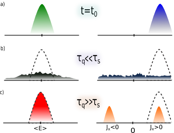
Figure 2: Scheme of the processes: probability distributions of the energy (left) and $J_{x}$ (right). a) Symmetry-breaking initial state, with mean energy $\left\langle E\right\rangle$ and $\left\langle J_{x}\right\rangle\neq 0$. b) A comparison between the initial distributions (dashed lines) and the final ones for a fast driving, and c) for a slow driving. If $\tau_{q}\ll\tau_{s}$, the energy is largely dissipated. If $\tau_{q}\gg\tau_{s}$ the energy distribution is fully recovered, but the process is irreversible since both modes are equally populated and therefore $\left<J_{x}\right>=0$.

III Results

III.1 Main result

The main result of the present article is sketched in Fig. 2. It can be summarized as follows:

If the driving is fast ($\tau_{q}/\tau_{s}\ll 1$) energy is largely dissipated and the final state is totally different from the initial one; this constitutes a standard irreversible process. On the contrary, if the driving is very slow ($\tau_{q}/\tau_{s}\gg 1$) the energy distribution is fully recovered; in other words, the total energy necessary to complete the cycle is zero, and all the mechanical work invested in the forward part is exactly recovered in the backwards. However, the distribution of the order parameter $J_{x}$ is dramatically changed. In the final state, this distribution is symmetric around zero, independently of the initial expectation value $\left\langle J_{x,i}\right\rangle$; it consists of two smaller copies of the initial one, centered at $J_{x}=\left\langle J_{x,i}\right\rangle$ and $J_{x}=-\left\langle J_{x,i}\right\rangle$, respectively. This entails the loss of the information about the initial symmetry-breaking, and can be quantified by the corresponding increase of the information entropy $I(J_{x})\sim\log 2$. Therefore, the process is irreversible despite the total absence of energy dissipation.

III.2 Unitary evolution with a coherent initial state

We explore the non-equilibrium dynamics of the system by means of a numerical simulation involving $N=500$ particles, where the estimated time scale results to be $\tau_{s}\simeq 0.01$. The presented results were obtained choosing a coherent state $\left|\mu=1/2\right\rangle$ as initial condition, and an equilibration time $t_{r}=9\times 10^{4}\tau_{s}$. The initial and final values of the external parameter are $\Lambda_{0}=7/2$ and $\Lambda_{1}=1/2$, respectively. To analyze different dynamical regimes as a function of the driving time, we study the expectation value of the first component of the Schwinger angular momentum $\left\langle J_{x}(t)\right\rangle$, and the probability distributions over $E_{i,n}$ and $J_{x}$, given by $\left|\left\langle E_{i},\pi_{n}\right|\left.\Psi(t)\right\rangle\right|^{2}=\left|C_{i,n}(t)\right|^{2}$ and $\left|\left\langle J,j_{x}\right|\Psi(t)\left.\right\rangle\right|^{2}=\left|K_{j_{x}}(t)\right|^{2}$ respectively, where $\left|E_{i},\pi_{n}\right>$ is an eigenstate of the Hamiltonian $H$, and $\left|J,j_{x}\right>$ an eigenstate of $J_{x}$, that is $J_{x}\left|J,j_{x}\right>=j_{x}\left|J,j_{x}\right>$.

The initial distributions corresponding to the initial state are represented in the Fig. 3. We plot the energy distribution before the protocol on the left, $\left|C_{i,n}(0)\right|^{2}$ (trivially, it remains unchanged between $t=0$ and $t=t_{r}$); the initial distribution of $J_{x}$, $\left|K_{j_{x}}(0)\right|^{2}$, in the middle, and the same distribution at $t=t_{r}$, after the system is equilibrated, on the right.

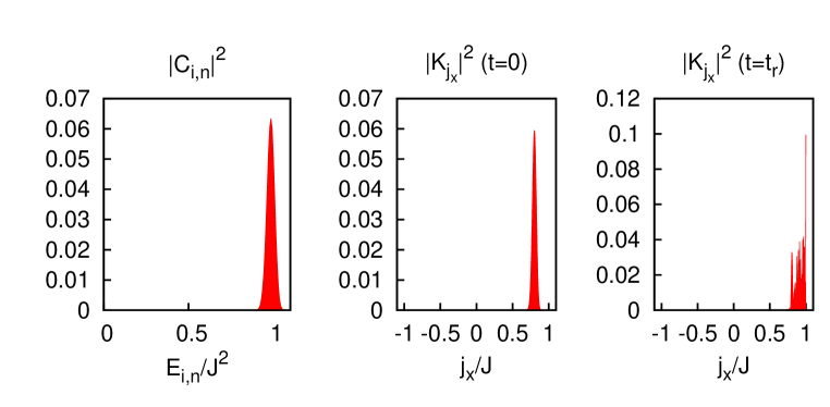
Figure 3: Probability distributions of the initial state. At the left, the energy distribution $\left|C_{i,n}(0)\right|^{2}$ is displayed. In the middle and at the right, the probability distributions over $J_{x}$, $\left|K_{j_{x}}(t)\right|^{2}$, at $t=0$ and $t=t_{r}$ are showed.

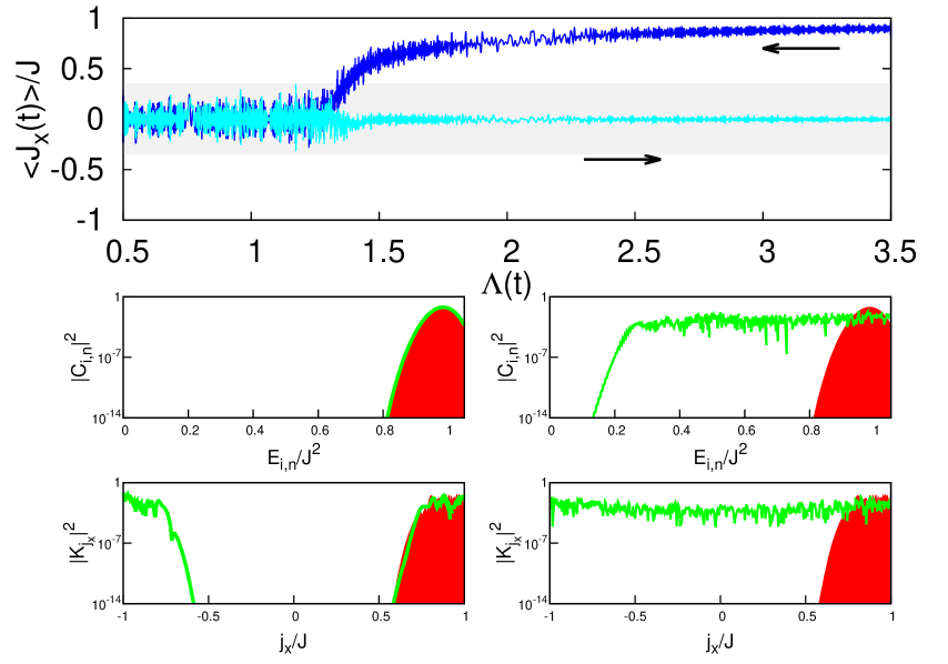
Figure 4: Results for two different dynamical regimes, left panels correspond to $\tau_{q}/\tau_{s}=7200$ while right panels correspond to $\tau_{q}/\tau_{s}=0.4$. At the top, time evolution of the expectation value $\left\langle J_{x}(t)\right\rangle$ as a function of the value of the external parameter $\Lambda(t)$. Forward and backward processes are plotted with dark and light lines (dark blue and cyan online) respectively. The arrows indicate the direction of the process starting at $\Lambda_{0}=7/2$. The gray band represents the possible final results for the slow protocol (see main text for more details). Middle and bottom rows, probability distribution of the energy and $J_{x}$. Filled region (red online) represents the initial probability distribution at $t=t_{r}$; solid lines (green online) the final at $t=2\tau_{q}+3t_{r}$.

In Fig. 4 we summarize our main results. In the upper part, the plot shows the time evolution of $\left\langle J_{x}(t)\right\rangle$ for the slow driving ($\tau_{q}/\tau_{s}=7200$) —the trajectory $\left\langle J_{x}(t)\right\rangle$ does not provide significative information for the fast driving ($\tau_{q}/\tau_{s}=0.4$), since the system is not equilibrated at intermediate times. In the panels below, we plot the main probability distributions, for the two paradigmatic regimes: at the left, for a slow driving ($\tau_{q}/\tau_{s}=7200$); at the right for a fast driving ($\tau_{q}/\tau_{s}=0.4$). In the middle panel, the energy distributions $\left|C_{i,n}(t)\right|^{2}$ are shown before (filled region) and after (solid lines) the cycle, in a logarithmic scale. In the lower panel, the probabilities $\left|K_{j_{x}}(t)\right|^{2}$ are plotted in the same format. It is clearly shown that the initial energy distribution is fully recovered at the end of the slow cycle. On the contrary, $\langle J_{x}(t)\rangle$ returns following a path totally different from the corresponding to the forward protocol. During the backward process, $\langle J_{x}(t)\rangle$ always fluctuates around a value close to zero, implying that the state consists of a superposition of the two symmetry-breaking branches, as it can be observed in the lower panel for $\left|K_{j_{x}}(t)\right|^{2}$. To get a deeper insight on this fact, we take into account that the equilibrium properties of the final state can be described by means of a long-time average at the fixed value $\Lambda_{0}$, from which we obtain the final equilibrium value $\overline{\left<J_{x,f}\right>}$. It is important to note that the returning path does not average exactly to $\overline{\left\langle J_{x,f}\right\rangle}=0$, but to a certain finite value depending on both the driving and the equilibration times, $\tau_{q}$ and $t_{r}$. We have performed several calculations with different equilibration times, which result in a region of possible final values of $\overline{\left<J_{x,f}\right>}$ at $\Lambda_{0}$, plotted as a band in the upper part of Fig. 4. Therefore, the final distribution of $J_{x}$ is not exactly symmetric in the majority of the cases and the superposition of the two branches is slightly biased towards the left or the right. Hence, for finite-size systems not all the information about the initial symmetry-breaking, but a very significant part of it, is lost as a consequence of the phase mixing between eigenstates of opposite parity once the state enters in the region without degeneracies. In Sec. III C we will show how the width of the band decreases as the number of initially populated eigenstates increases, suggesting that the band tends to shrink to $\overline{\left\langle J_{x}\right\rangle}=0$ in the thermodynamic limit. Furthermore, in Sec. V we will give theoretical arguments supporting this conclusion. Although not explicitly shown, the same final state is obtained independently of the degree of symmetry-breaking of the initial condition.

On the other hand, the fast protocol corresponds to a standard irreversible process, with measurable consequences in any observable. In particular, the final distribution for the energy is totally different from the initial one. A thermodynamic interpretation of this fact can be done in the following terms. The energy variation in a process done in a quantum isolated system $\Lambda_{i}\rightarrow\Lambda_{f}$ can be divided in two parts: $\Delta E=W+Q$, with $W=\sum_{j}p_{j}^{i}\left[E_{j}\left(\Lambda_{f}\right)-E_{j}\left(\Lambda_{i}\right)\right]$, and $Q=\sum_{j}\left[p_{j}^{f}-p_{j}^{i}\right]E_{j}\left(\Lambda_{f}\right)$, being $E_{j}(\Lambda)$ the j-th energy level of $H(\Lambda)$, and $p_{j}^{i}$ and $p_{j}^{f}$ the population of that energy level in the initial (before the protocol) and in the final state (after completing the protocol), respectively. $W$ can be understood as the reversible work done in the system, and $Q$ as the dissipated heat as a consequence of the protocol Polkovnikov:08 . $W$ represents the energy change due to the change in the energy levels $E_{j}(\Lambda_{i})\rightarrow E_{j}(\Lambda_{f})$, which only depends on the initial and final values of the external parameter of the Hamiltonian. On the other hand, $Q$ represents the change in the energy due of the non-adiabatic transitions between energy levels; this is the reason why it can be understood as the heat dissipated by the protocol, despite the system is always isolated from any external environment. Therefore, if the energy distribution remains unchanged after a cyclic process, that is, the population of all the energy levels is the same in the initial and the final states, $p_{j}^{f}=p_{j}^{i}$ $\forall j$, the mechanical work invested in the forward process is exactly retrieved in the backward, and therefore the process is usually understood as reversible. On the contrary, any change in the energy distribution after a cyclic process implies that some of this mechanical work has been dissipated into heat, meaning that the population of the energy levels has changed $p_{j}^{f}\neq p_{j}^{i}$ and hence the process is irreversible (see Sec. IV for a link between this dissipated energy and the von Neumann entropy of the equilibrium states). Furthermore, in this last case (fast driving protocol) as we can see in Fig. 4 (or in Fig. 5 for additional initial states), the final distribution of $J_{x}$ is also totally different from the initial one. First, it is symmetric, implying that $\left<Jx\right>=0$, as it also happens as a consequence of the slow driving. Second, it is much wider, with a shape totally different from the initial one; it does not consist of the superposition of two modes, but to a roughly flat distribution between $J_{x}=-J$ and $J_{x}=J$, which is a consequence of the energy dissipation of the process.

III.3 Additional initial states

We provide additional results with different initial symmetry-breaking states. The mean spacing of the spectrum at $\Lambda_{0}=7/2$ is $\bar{E}/J^{2}\simeq 0.003$, which turns out to be an useful quantity to compare the width of the states. Here, we define three different initial states to support the previous conclusions based on the driving process starting with a coherent state $\left|\mu=1/2\right\rangle$. In all of them only one mode is populated and therefore the population imbalance is maximum with $\left\langle J_{x}\right\rangle\simeq J$:

• Rectangular: An initial state that just populates the last $50$ double-degenerated eigenstates ($M=25$ doublets) of the Hamiltonian with the same probability, i.e. $\left|C_{i,n}\right|_{R}^{2}=1/(2M)$ for the last $2M=50$ eigenstates $\left|E_{i},\pi_{n}\right\rangle$, and $\left|C_{i,n}\right|_{R}^{2}=0$ for the rest.

• Gaussian: An initial state that populates the eigenstates with a Gaussian probability, whose mean energy value is $\tilde{\mu}_{1G}/J^{2}=\left\langle E_{1G}\right\rangle/J^{2}=0.922$, and variance $\sigma_{1G}/J^{2}=0.035\simeq 10\bar{E}/J^{2}$. Therefore, an eigenstate $\left|E_{i},\pi_{n}\right\rangle$ will be populated according to $\left|C_{i,n}\right|_{1G}^{2}\propto e^{-\frac{\left(E_{i,n}-\mu_{1G}\right)^{2}}{2\sigma_{1G}^{2}}}$.

• Double-Gaussian: An initial state that consists of two separated Gaussian probability distributions. Both have the same variance $\sigma_{2G}/J^{2}=0.017\simeq 5\bar{E}/J^{2}$ but different mean energy, which are $\tilde{\mu}_{2G_{1}}/J^{2}=0.971$ and $\tilde{\mu}_{2G_{2}}/J^{2}=0.805$. Therefore $\left\langle E_{2G}\right\rangle/J^{2}\simeq 1/2\left(\tilde{\mu}_{2G_{1}}+\tilde{\mu}_{2G_{2}}\right)=0.888$. Hence, an eigenstate $\left|E_{i},\pi_{n}\right\rangle$ will be populated according to $\left|C_{i,n}\right|_{2G}^{2}\propto e^{-\frac{\left(E_{i,n}-\mu_{2G_{1}}\right)^{2}}{2\sigma_{2G}^{2}}}+e^{-\frac{\left(E_{i,n}-\mu_{2G_{2}}\right)^{2}}{2\sigma_{2G}^{2}}}$.

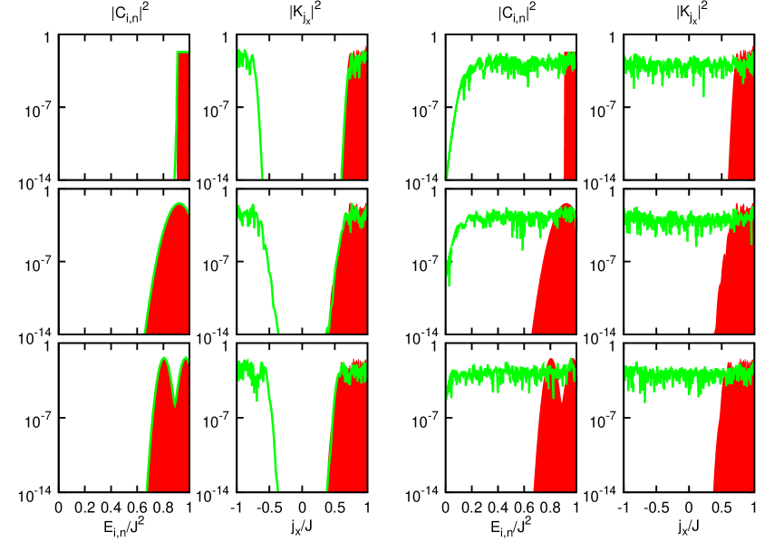
Figure 5: Results for two different dynamical regimes for additional initial states, the two columns at the left correspond to a slow driving ($\tau_{q}/\tau_{s}=1538$), whereas the two columns at the right correspond to a fast driving ($\tau_{q}/\tau_{s}=0.2$). The results for rectangular, Gaussian and double-Gaussian are plotted in the first, second and third row respectively. For each driving process, we represent the probability distribution of the energy (left) and of the $J_{x}$ (right) in logarithmic scale. The filled region (red online) represents the initial probability distribution at $t=t_{r}$, while solid lines (green online) the final at $t=2\tau_{q}+3t_{r}$.

After performing a protocol for each additional initial state, we obtain the results summarized in the different panels of the Fig. 5. Each row corresponds to a different initial state, rectangular (top), Gaussian (middle) and double-Gaussian (bottom). For each case, a fast ($\tau_{q}/\tau_{s}=0.2$) and a slow ($\tau_{q}/\tau_{s}=1538$) protocol are presented. As we have already showed in the previous section, while for the slow protocol the energy distribution is completely recovered and the probability distribution over $J_{x}$ is split in the two possible branches ($\left<J_{x}\right>\lessgtr 0$), for a fast protocol neither the $J_{x}$-distribution nor the energy are recovered, which implies large dissipation.

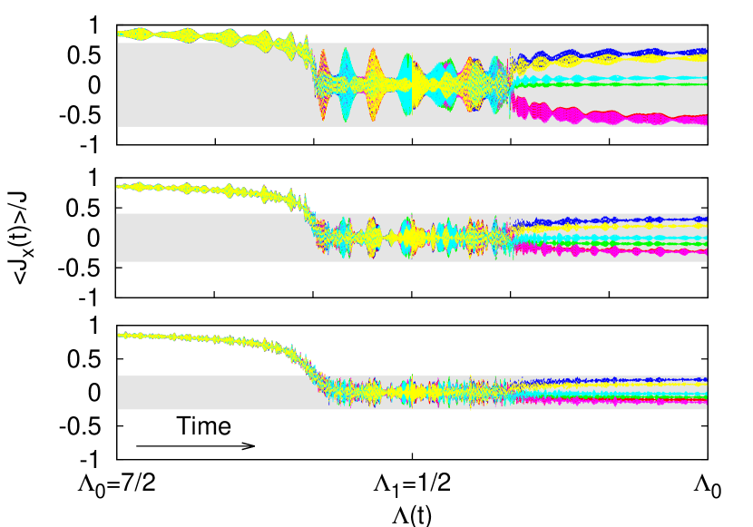
Figure 6: Expectation value $\left<J_{x}(t)\right>$ as a function of the time-dependent control parameter $\Lambda(t)$ for Gaussian initial states with different variances: $\sigma\simeq 2.3\bar{E}$ (top), $\sigma\simeq 7\bar{E}$ (middle) and $\sigma\simeq 16.3\bar{E}$ (bottom), but same mean energy. For each Gaussian initial state, we perform six cycles with slightly different values of $\tau_{q}$ times (from $\tau_{q}/\tau_{s}=1500$ to $\tau_{q}/\tau_{s}=1505$) plotted with different colors. For all the cases, the initial value $\left<J_{x}(t=0)\right>\simeq J$, whereas the possible final results are encoded by a gray band. Clearly, the wider the initial state, the narrower the gray band.

Finally, we perform different cycles for three Gaussian initial states with the same mean energy but different variances, in order to study how the width of the band shown in the upper part of Fig. 4 depends on the number of initially populated double-degenerated eigenstates. We consider three Gaussians with variances $\sigma\simeq 2.3\bar{E},7\bar{E}$ and $16.3\bar{E}$, respectively. Then, we perform slow cycles with slightly different values of $\tau_{q}$ to obtain the possible final results of the expectation value of the observable $J_{x}$, ensuring that the energy distribution is recovered. The results are summarized in the Fig. 6. There, the narrowest Gaussian initial state (top) generates a broad region of possible final expectation values $\left<J_{x}\right>$, which means that the protocol can end in a state very similar to the initial condition. On the other hand, the widest Gaussian initial state (bottom) provides a narrow band, since the number of initially populated eigenstates is considerably larger. This entails that the protocol always ends with an almost perfect superposition of the two symmetry-breaking branches. Clearly, the wider the initial state, the narrower the gray band of the possible final results, and hence is reasonable to conjecture that the band shrinks to zero, and then, the final expectation value $\left<J_{x}\right>\rightarrow 0$ in the thermodynamic limit. This fact will be confirmed with theoretical arguments in the Sec. V.

IV Entropy and information

As the state of the system is always pure, we cannot link this source of irreversibility to a (thermodynamic) entropy production. To develop a thermodynamic interpretation, we rely on initial (before the protocol) and intermediate (before the backward process) equilibrium states, which are the key elements of the Crook’s theorem Talkner:08 ; Crooks:98 . It has been recently shown that these equilibrium states exist for (almost) any isolated quantum system unitary evolving after (almost) any initial condition, and they coincide with the long-time average, $\rho_{\text{eq}}=\lim_{T\rightarrow\infty}\frac{1}{T}\int_{0}^{T}dt\,\left|\Psi(t)\right>\left<\Psi(t)\right|$ Reimann:12 —the actual state $\left|\Psi(t)\right\rangle$ fluctuates around this equilibrium state, remaining close to it during the majority of the time. Note that this is just a formal definition, meaning a very long time average keeping fixed all the free parameters of the Hamiltonian. In our case, it has to be understood as a time average of the state evolving under $H(\Lambda)$, with a fixed value of $\Lambda$, not to an average over the whole protocol $\Lambda(t)$.

From this equilibrium state, we calculate $\Delta S=S(\Lambda_{1})-S(\Lambda_{0})$, being $S=-\text{Tr}\left[\rho_{\text{eq}}\log\rho_{\text{eq}}\right]$ the von Neumann entropy of these reference states. We compare this value with the dissipated energy, $\left\langle E_{\text{dis}}\right\rangle=\left\langle E_{\text{final}}\right\rangle-\left\langle E_{\text{initial}}\right\rangle$. Results are plotted in Fig. 7, where the circles represent the dissipated energy $\left|\left\langle E_{\text{dis}}\right\rangle\right|/\left\langle E_{\text{initial}}\right\rangle$ and the squares the increment of entropy $\Delta S$, as a function of the driving time $\tau_{q}/\tau_{s}$. When this time is short, $\tau_{q}\ll\tau_{s}$, the energy is largely dissipated, due to the non-adiabatic transitions between energy levels, as it is discussed in Sec. III; hence, the increment of entropy is substantial. The number of these non-adiabatic transitions diminishes with the increase of the driving time $\tau_{q}$, decreasing the von Neumann entropy in a similar rate. Finally, if $\tau_{q}\gg\tau_{s}$, there is no dissipated energy, but the final entropy is still larger than the initial one, $\Delta S=\log 2$.

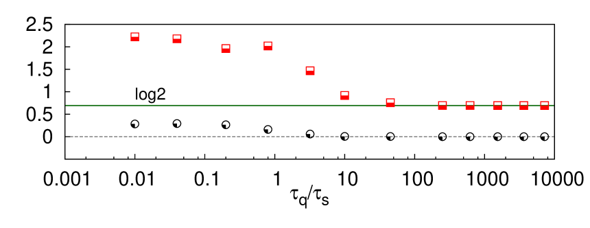
Figure 7: Increment of the von Neumann entropy $\Delta S$ between the initial state and the equilibrium state after the forward process with squares (red online), as a function of the driving time $\tau_{q}/\tau_{s}$. The circles (black online) illustrate the dissipated energy $\left|\left\langle E_{\text{dis}}\right\rangle\right|/\left\langle E_{\text{initial}}\right\rangle$.

This result contradicts the common thermodynamic lore, based on a direct link between entropy production and energy dissipation. From Figs. 4 and 7 we infer that, for slow enough processes $\tau_{q}\gg\tau_{s}$, the probability of investing a certain work $w$ in the forward process, $P_{f}(w)$, is exactly the same than the probability of recovering the same magnitude of work $-w$ in the backwards $P_{b}(w)$, that is, $P_{f}(w)/P_{b}(-w)=1$. This implies that any measurement of the dissipated work $w_{\text{dis}}$ in the complete protocol, which can experimentally performed following the strategy very recently proposed in Roncaglia:14 , gives $w_{\text{dis}}=0$; the population of all energy levels remains unchanged, no heat is produced and all the work done in the forward part of the protocol is retrieved in the backwards. On the contrary, a similar measurement performed on the observable $J_{x}$, which can be experimentally done following Zibold:10 , gives an opposite result: the probability of obtaining the same value $j_{x}$ is not the same at the beginning and at the end of the protocol, $P_{f}(j_{x})\neq P_{i}(j_{x})$.

To obtain a physical interpretation of this fact, we consider the information entropy of an observable $A$, defined as $I\left(A\right)=-\sum_{n}p_{n}\log p_{n}$, being $p_{n}$ the probability of obtaining the eigenvalue $A_{n}$ in a measurement. From the previous results it is clear that $\Delta I(H)\rightarrow 0$ when $\tau_{q}\gg\tau_{s}$. On the contrary, $\Delta I(J_{x})\sim\log 2$  when $\tau_{q}\gg\tau_{s}$. Hence, the main consequence of the protocol is a loss of information about $J_{x}$ which equals the increase of the von Neumann entropy of the long time-average state, despite the absence of dissipation. This constitutes an unexpected source of irreversibility.

A qualitative explanation of this fact can be done in the following terms. The direct link between entropy production and energy dissipation is established considering that the final equilibrium value after any thermodynamic process, $\rho_{\text{eq}}$, is given by a density matrix which is diagonal in the basis that diagonalizes the CSCO Polkovnikov:11b . The precise shape of this matrix is determined by all the relevant conserved quantities of the Hamiltonian Polkovnikov:11 . In our case, the only global constant of motion for any value of the coupling parameter $\lambda$ is the parity $\Pi$. Hence, at a first sight, the equilibrium state $\rho_{\text{eq}}$ should be diagonal in the eigenbasis which diagonalizes the $\{H,\Pi\}$, that we label $\left|E_{i},\pm\right>$. However, there exists another operator which remains constant only above the critical energy of the ESQPT, the coherences between the two parity sectors of the Hamiltonian $C=\sum_{i}\left|E_{i},+\right>\left<E_{i},-\right|+h.c.$ The key point is that this operator has no diagonal elements in the eigenbasis of $\{H,\Pi\}$, and hence any information regarding its initial value is encoded in the non-diagonal part of the initial equilibrium state. This information is kept by the protocol only if the system remains above the critical energy of the ESQPT; as soon as the protocol leads the system to $E<E_{c}$, $C$ ceases to be a constant of motion and all the information about its initial value is erased by phase mixing. As a consequence, $\rho_{\text{eq}}$ changes from non-diagonal in the initial state, to diagonal in the final equilibrium state, leading $\Delta S=\log 2$. And, as we have pointed before, this irreversible change persists even when the protocol is performed slow enough to avoid non-adiabatic transitions between energy subspaces, and therefore constitutes a source of irreversibility independent of the energy dissipation.

V Mechanism of irreversibility

The microscopic origin of this kind of irreversibility is the collective phase mixing in the normal phase. The effect of the intrinsic irreversibility due to the loss of information is remarkable when the process is performed slow enough to prevent transitions between different energy levels, that is, when the system evolves in the quasistatic limit. Hence, the wave function can be expressed as $\left|\Psi(t)\right\rangle=\sum_{i,n}e^{-i\phi_{i,n}(t)}\Gamma_{i,n}\left|E_{i},\pi_{n}\right\rangle$, where $\Gamma_{i,n}$ are the coefficients of the initial wavefunction in the eigenstates of $H\left(\Lambda_{0}\right)$, and $\left|E_{i},\pi_{n}\right\rangle$ are the common eigenstates of the instantaneous Hamiltonian $H\left(\Lambda(t)\right)$ and the parity $\Pi$. Therefore, the only relevant change in the wave-function due to the time-dependent protocol $\Lambda(t)$ resides in the phases $\phi_{i,n}=\theta_{i,n}+\gamma_{i,n}$. The first term $\theta_{i,n}$ accounts for the dynamical phase, $\theta_{i,n}(t)=\int_{0}^{t}d\tau E_{i,n}(\tau)$. The second one represents the geometrical Berry phase, $\gamma_{i,n}=-i\int_{\Lambda_{i}}^{\Lambda_{f}}\left\langle E_{i},\pi_{n}(\Lambda)\right|\partial_{\Lambda}\left|E_{i},\pi_{n}(\Lambda)\right\rangle d\Lambda$, where the dependence on $\Lambda$ of the instantaneous eigenstates $\left|E_{i},\pi_{n}\right>$ is explicitly shown. As our protocol consists in just changing one parameter with the same initial and final states $\Lambda_{i}\rightarrow\Lambda_{f}\rightarrow\Lambda_{i}$, the net contribution of the Berry phase is zero, and hence the only relevant term is the dynamical phase $\phi_{i,n}=\theta_{i,n}$. At the end of the cycle, the value of this phase is

$$\phi_{i,n}=\frac{2\tau_{q}}{\Lambda_{1}-\Lambda_{0}}\int_{\Lambda_{0}}^{\Lambda_{1}} d\Lambda E_{i,n}(\Lambda)+$$ (3)

$$+ t_{r}\left[2E_{i,n}\left(\Lambda_{0}\right)+E_{i,n}\left(\Lambda_{1}\right)\right].$$

To evaluate the changes in the wavefunction due to the protocol $\Lambda_{0}\rightarrow\Lambda_{1}\rightarrow\Lambda_{0}$, we study how the initial and final states evolve under $H(\Lambda_{0})$. In this case, the initial and the final time-dependent wavefunctions are

$$\left|\Psi_{i}(t)\right> = \sum_{j,n}\text{e}^{-iE_{j,n}t}\Gamma_{j,n}\left|E_{j},\pi_{n}\right>;$$ (4)

$$\left|\Psi_{f}(t)\right> = \sum_{j,n}\text{e}^{-i\phi_{j,n}}\text{e}^{-iE_{j,n}t}\Gamma_{j,n}\left|E_{j},\pi_{n}\right>.$$ (5)

So, the initial and final expectation values of any observable $O$ measured under such circumstances are

$$\left<O_{i}(t)\right>=\sum_{kj}\sum_{nm} \text{e}^{-i(E_{k,n}-E_{j,m})t}\times$$ (6)

$$\times \Gamma^{*}_{j,m}\Gamma_{k,n}\left<E_{j},\pi_{m}\right|O\left|E_{k},\pi_{n}\right>;$$

$$\left<O_{f}(t)\right>=\sum_{kj}\sum_{nm} \text{e}^{-i(\phi_{k,n}-\phi_{j,m})}\text{e}^{-i(E_{k,n}-E_{j,m})t}\times$$ (7)

$$\times \Gamma^{*}_{j,m}\Gamma_{k,n}\left<E_{j},\pi_{m}\right|O\left|E_{k},\pi_{n}\right>.$$

These expressions give the exact time evolution of $\langle O\rangle$ before and after completing the protocol. As we have previously shown, these time-dependent expectation values fluctuate around the corresponding equilibrium values, $\overline{\left\langle O_{i}\right\rangle}$ and $\overline{\left\langle O_{f}\right\rangle}$, given in both cases by the long-time average under the same Hamiltonian $H(\Lambda_{0})$, $\overline{\left\langle O\right\rangle}=\lim_{T\rightarrow\infty}\frac{1}{T}\int_{0}^{T}dt\left<O(t)\right>$. Hence, to obtain a simple interpretation of the results, we follow the reasoning in terms of these equilibrium values, which are given by

$$\overline{\left\langle O_{i}\right\rangle} = \sum_{kj}\sum_{nm}\Gamma^{*}_{j,m}\Gamma_{k,n}\left<E_{j},\pi_{m}\right|O\left|E_{k},\pi_{n}\right>\times$$ (8)

$$\times \lim_{T\rightarrow\infty}\frac{1}{T}\int_{0}^{T}dt\text{e}^{-i(E_{k,n}-E_{j,m})t};$$

$$\overline{\left\langle O_{f}\right\rangle} = \sum_{kj}\sum_{nm}\text{e}^{-i(\phi_{k,n}-\phi_{j,m})}\Gamma^{*}_{j,m}\Gamma_{k,n}\left<E_{j},\pi_{m}\right|O\left|E_{k},\pi_{n}\right>\times$$ (9)

$$\times \lim_{T\rightarrow\infty}\frac{1}{T}\int_{0}^{T}dt\text{e}^{-i(E_{k,n}-E_{j,m})t}.$$

Since $\Lambda_{0}$ lies on the degenerate phase, we can consider that $E_{i,+}=E_{i,-}$, where $+$ ($-$) denotes the positive (negative) parity sector. So, after the time average is performed, only diagonal and non-diagonal terms connecting $\left|E_{i},+\right>$ with $\left|E_{i},-\right>$ survive. Therefore, the initial and final equilibrium values are

$$\overline{\left\langle O_{i}\right\rangle} = \sum_{j}\left|\Gamma_{j,+}\right|^{2}\left<E_{j},+\right|O\left|E_{j},+\right>+$$

$$+ \sum_{j}\left|\Gamma_{j,-}\right|^{2}\left<E_{j},-\right|O\left|E_{j},-\right>+$$

$$+ \sum_{j}\left(\Gamma_{j,+}^{*}\Gamma_{j,-}\left<E_{j},+\right|O\left|E_{j},-\right>+h.c.\right);$$

$$\overline{\left\langle O_{f}\right\rangle} = \sum_{j}\left|\Gamma_{j,+}\right|^{2}\left<E_{j},+\right|O\left|E_{j},+\right>+$$

$$+ \sum_{j}\left|\Gamma_{j,-}\right|^{2}\left<E_{j},-\right|O\left|E_{j},-\right>+$$

$$+ \sum_{j}\left(\Gamma_{j,+}^{*}\Gamma_{j,-}\text{e}^{-i\left(\phi_{j,+}-\phi_{j,-}\right)}\left<E_{j},+\right|O\left|E_{j},-\right>+h.c.\right).$$

The phases affecting the non-diagonal part of the time average can be written

$$\phi_{j,+}-\phi_{j,-} = \frac{2\tau_{q}}{\Lambda_{1}-\Lambda_{0}}\int_{\Lambda_{0}}^{\Lambda_{1}}d\Lambda\left[E_{j,+}(\Lambda)-E_{j,-}(\Lambda)\right]+$$ (12)

$$+ t_{r}\left[E_{j,+}\left(\Lambda_{1}\right)-E_{j-}\left(\Lambda_{1}\right)\right]\equiv\omega_{j}.$$

As it is obvious from this equation, the phases $\omega_{j}=\omega_{j}(\tau_{q},t_{r})$ depend on both the driving time, $\tau_{q}$, and the equilibration time, $t_{r}$, though this dependence is not explicitly written to simplify the notation.

A logical consequence of this fact is that the expected value of any observable commuting with $\Pi$ is the same at the initial and the final stages of the protocol. In particular, this happens for the projector over any eigenstate, and hence the energy distribution remains unchanged by the protocol. On the other hand, the result for $J_{x}$ is

$$\overline{\left\langle J_{x,i}\right\rangle} = \sum_{j}\left(e^{-i\beta_{j}}\left|\Gamma_{j,\pm}\right|\left<E_{j},+\right|J_{x}\left|E_{j},-\right>+h.c.\right)$$ (13)

$$\overline{\left\langle J_{x,f}\right\rangle} = \sum_{j}\left(\text{e}^{-i(\omega_{j}+\beta_{j})}\left|\Gamma_{j,\pm}\right|\left<E_{j},+\right|J_{x}\left|E_{j},-\right>+h.c.\right),$$

where $\left|\Gamma_{j,\pm}\right|e^{-i\beta_{j}}=\Gamma_{j,+}^{*}\Gamma_{,j-}$. Hence, for slow enough processes, the only consequence at the end of the cycle is a set of phases $\omega_{j}$ arising for each doublet, giving rise to $\overline{\left\langle J_{x,f}\right\rangle}=2\sum_{j}\cos(\omega_{j}+\beta_{j})\left|\Gamma_{j,\pm}\right|\left<E_{j},+\right|J_{x}\left|E_{j},-\right>$. The exact value of this sum depends on the initial condition, the details of the protocol and the expected values $\left<E_{j},+\right|J_{x}\left|E_{j},-\right>$, so a numerical diagonalization of the quantum problem is required. However, a good estimate can be obtained under certain assumptions. First, consider that the initial condition has only real coefficients, $\beta_{j}=n\pi,n=0,1,2,\ldots,\,\forall j$, and suppose that a mechanism similar to the Eigenstate Thermalization Hypothesis Srednicki:94 ; Rigol:08 holds, implying $\left<E_{j,+}\right|J_{x}\left|E_{j,-}\right>\sim J_{x}^{\text{ETH}}$ for all the $M$ populated eigenspaces; this entails that

$$\overline{\left\langle J_{x,f}\right\rangle}=2J_{x}^{\text{ETH}}\sum_{j}^{M}\cos\omega_{j}\cos\beta_{j}\left|\Gamma_{j,\pm}\right|.$$ (14)

Second, let’s consider that the dynamical phases $\omega_{j}$ and the coefficients $\cos\beta_{j}\left|\Gamma_{j,\pm}\right|$ behave as uncorrelated random variables . For two uncorrelated random variables $X$ and $Y$, $\langle XY\rangle=\langle X\rangle\langle Y\rangle$, being $\langle\rangle$ the statistical average, and thus $\sum_{j=1}^{M}X_{j}Y_{j}=M\langle XY\rangle=M\langle X\rangle\langle Y\rangle=(1/M)\sum_{j=1}^{M}X_{j}\sum_{j=1}^{M}Y_{j}$. Applying this result we obtain

$$\overline{\left\langle J_{x,f}\right\rangle}=\frac{2J_{x}^{\text{ETH}}}{M}\sum_{j}^{M}\cos\beta_{j}\left|\Gamma_{j,\pm}\right|\sum_{j}^{M}\cos\omega_{j}.$$ (15)

Finally, considering that the initial equilibrium value is $\overline{\left\langle J_{x,i}\right\rangle}=2J_{x}^{\text{ETH}}\sum_{j}\cos\beta_{j}\left|\Gamma_{j,\pm}\right|$, we conclude that

$$\overline{\left\langle J_{x,f}\right\rangle}=\frac{\overline{\left\langle J_{x,i}\right\rangle}}{M}\sum_{j}^{M}\cos\omega_{j}.$$ (16)

Two important physical conclusions arise from this result. First, $\left|\overline{\left\langle J_{x,f}\right\rangle}\right|\leq\left|\overline{\left\langle J_{x,i}\right\rangle}\right|$ for any initial state satisfying the previous conditions and for any slow-enough process. This entails that, if $\sum_{j}^{M}\cos(\omega_{j})<M$ for any value of $\tau_{q}$ and $t_{r}$, the protocol turns out to be irreversible, because $\overline{\left\langle J_{x,i}\right\rangle}$ is not recovered at the end. Moreover, if the phases $\omega_{j}$ are different for every doublet, we can expect that $\sum_{j}^{M}\frac{\cos\omega_{j}}{M}\sim 0$, provided the initial state is spread over a large enough number of eigenstates of the initial Hamiltonian, as it happens in the thermodynamic limit. So, in any case a relevant part of the information about the initial symmetry-breaking, encoded in the initial value $\overline{\left\langle J_{x,i}\right\rangle}$, is irreversibly lost after the protocol. For a clear interpretation of this result, it is worth to have in mind that the choice of the time-dependent protocol $\Lambda(t)$ constitutes an one degree of freedom macroscopic trajectory, which produces a very large number of different microscopic phases. Therefore, to exactly revert the process $H(t)\rightarrow H(-t)$, a Maxwell’s demon-like machine Muruyama:09 with a fully microscopic knowledge of the system is required, exactly as for any other thermodynamic irreversible phenomenon.

On the other hand, if the initial state only populates one doublet, the final result is $\overline{\left\langle J_{x,f}\right\rangle}=\overline{\left\langle J_{x,i}\right\rangle}\cos\omega_{m}(\tau_{q},t_{r})$. This implies that the final equilibrium value $\overline{\left\langle J_{x,f}\right\rangle}$ oscillates between $-\overline{\left\langle J_{x,i}\right\rangle}$ and $\overline{\left\langle J_{x,i}\right\rangle}$, depending on the precise values of $\tau_{q}$ and $t_{r}$. Hence, the information about the initial symmetry-breaking is not lost at all after the forward process, as it happens if the initial state populates a large number of doublets —the initial value $\overline{\left\langle J_{x,i}\right\rangle}$ can be easily recovered selecting $t_{r}$ in the normal phase to make $\omega_{m}(\tau_{q},t_{r})=2\pi n$, being $n=0,1,2,\ldots$. The main difference between this and the previous case is that the protocol gives rise to a single phase $\omega_{m}(\tau_{q},t_{r})$ in this one, which can be removed by means of a precise choice of $t_{r}$ and $\tau_{q}$.

For small systems, in which only a small number of doublets are populated in the initial state, we can have a intermediate result with $\overline{\left\langle J_{x,f}\right\rangle}$ oscillating between $-\hat{J}$ and $\hat{J}$. This is what we plot as a band in Fig. 4, being $\hat{J}$ smaller as the number of initially populated doublets is increased, as we show in Fig. 6. The exact value of $\overline{\left\langle J_{x,f}\right\rangle}$ depends on the precise values of the phases $\omega_{j}$, but we can expect that almost any protocol gives rise to a quite large number of different phases $\omega_{j}$, at least if the system is large enough to have a large number of doublets populated in the initial state, and hence $\overline{\left\langle J_{x,f}\right\rangle}\sim 0$.

VI Conclusions

In this article we report the existence of irreversible processes without energy dissipation in a certain kind of isolated quantum systems. Starting with a symmetry-breaking state in which only one of the two symmetry-breaking branches is populated, and changing a system parameter slowly enough, we perform a closed cycle which is quasistatic —the initial energy distribution is perfectly recovered at the end, and hence the net work necessary to complete the cycle is zero. However, the process results to be irreversible, because the final equilibrium state consists of a superposition of the two symmetry-breaking branches, no matters the fine details of the initial condition. So, this kind of irreversibility is not related to the dissipation of energy, but to an unavoidable loss of information, which is caused by the collective phase mixing between different symmetry sectors when the system enters in a phase with no degeneracies. This phase mixing entails the unavoidable erasure of the information about the initial symmetry-breaking, making the process irreversible, no matters how slow it is performed. We exemplify this fact by means of numerical calculations in an experimental feasible many-body quantum system, which is a special case of the Lipkin-Meshkov-Glick model. We perform an irreversible cycle consisting of a unitary time evolution that entails a loss of information $\Delta I\sim\log 2$ in the measurement of a symmetry-breaking observable, that we identify with an increase of the von Neumann entropy of the long-time average equilibrium states, that tends to $\Delta S=\log 2$ in the quasistatic limit.

- (1) C. Jarzynski, Annu. Rev. Cond. Matter Phys. 2, 329 (2011); M. Campisi, P. Hänggi, and P. Talkner, Rev. Mod. Phys. 83, 771 (2011).
- (2) P. Talkner, P. Hänggi, and M. Morillo, Phys. Rev. E 77, 051131 (2008).
- (3) L. Szilard, Z. Phys. A 53, 840 (1929).
- (4) R. Landauer, IBM J. Res. Dev. 5, 183 (1961).
- (5) T. Sagawa and M. Ueda, Phys. Rev. Lett. 104, 090602 (2010).
- (6) J. M. Horowitz and H. Sandberg, New. J. Phys. 16, 125007 (2014).
- (7) A. Polkovnikov, K. Sengupta, A. Silva, and M. Vengalattore, Rev. Mod. Phys. 83, 863 (2011).
- (8) M. Rigol, V. Dunjko, V. Yurovsky, and M. Olshanii, Phys. Rev. Lett. 98, 050405 (2007).
- (9) R. Puebla, A. Relaño, and J. Retamosa, Phys. Rev. A 87, 023819 (2013).
- (10) R. Puebla, and A. Relaño, Europhys. Lett. 104, 50007 (2013).
- (11) T. Zibold, E. Nicklas, C. Gross, and M. K. Oberthaler, Phys. Rev. Lett. 105, 204101 (2010).
- (12) C. Gross, T. Zibold, E. Nicklas, J. Esteve, and M. K. Oberthaler, Nature (London) 464, 1165 (2010).
- (13) H. J. Lipkin, N. Meshkov, and A. J. Glick, Nucl. Phys. 62, 188 (1965).
- (14) J. Vidal, G. Palacios, and R. Mosseri, Phys. Rev. A 69, 022107 (2004); S. Dusuel, and J. Vidal, Phys. Rev. Lett. 93, 237204 (2004); P. Ribeiro, J. Vidal, and R. Mosseri, Phys. Rev. Lett. 99, 050402 (2007); P. Ribeiro, J. Vidal, and R. Mosseri, Phys. Rev. E 78, 021106 (2008).
- (15) A. Relaño, J. M. Arias, J. Dukelsky, J. E. García-Ramos, and P. Pérez-Fernández, Phys. Rev. A 78, 060102(R) (2008); P. Pérez-Fernández, A. Relaño, J. M. Arias, J. Dukelsky, and J. E. García-Ramos, Phys Rev. A 80, 032111 (2009).
- (16) T. Caneva, R. Fazio, and G. E. Santoro, Phys. Rev. B 78, 104426 (2008).
- (17) A. Polkovnikov, Phys. Rev. Lett. 101, 220402 (2008)
- (18) G. E. Crooks, J. Stat. Phys. 90, 1481; G. E. Crooks, Phys. Rev. E 60, 2721.
- (19) P. Reimann and M. Kastner, New. J. Phys. 14, 043020 (2012).
- (20) M. Srednicki, Phys. Rev. E 50, 888 (1994).
- (21) M. Rigol, V. Dunjko, and M. Olshanii, Nature 452, 854 (2008).
- (22) K. Muruyama, F. Nori, and V. Vedral, Rev. Mod. Phys. 81, 1 (2009).
- (23) A. J. Roncaglia, F. Cerisola, and J. P. Paz, Phys. Rev. Lett. 113, 250601 (2014).
- (24) A. Polkovnikov, Ann. Phys. (N. Y.) 326, 486 (2011).