Interference in a two-mode Bose system with $N$ particles is typical

Abstract

When a Bose-Einstein condensate is divided into two parts, that are subsequently released and overlap, interference fringes are observed. We show here that this interference is typical, in the sense that most wave functions of the condensate, randomly sampled out of a suitable ensemble, display interference. We make no hypothesis of decoherence between the two parts of the condensates.

I Introduction

The experimental observation of Bose-Einstein condensation raised a number of deep questions regarding the phase of the condensate and its operational meaning, its interference properties and other quantum concepts PW ; SB ; Leggett ; BDZ ; PS ; PeSm ; Leggettbook . Interference fringes are observed when two independently prepared Bose-Einstein condensates (BECs) are released and overlap exptBEC . At first sight, this phenomenon seems to be in contrast with commonly accepted wisdom on the Young-type double-slit interference (first-order interference) experiments from independent sources: since the relative phase between the two wave functions is not constant (this is what is meant by “independent” sources), no interference can be observed. Notice however that the second-order (two-particle) interference can be observed in a Hanbury-Brown and Twiss type experiment HBT1 ; HBT , where the quantum interference between the amplitudes corresponding to the two paths from the independent sources to the detectors is observed feynman ; ref:Loudon ; ref:MandelWolf .

Questions on the interference and the phase of the condensate have attracted the attention of many researchers. This motivated a very interesting debate on the most fundamental aspects of quantum mechanics and the features of many-body quantum systems. Javanainen and Yoo JY proposed that the phase of the condensate is established by measurement: an interference pattern is certainly observed in each single experimental run, but the patterns shift from run to run, so that no interference persists if all the observed interference patterns are superimposed, with no contradiction with the common wisdom on the first-order interference. The conclusion that the phenomenon can be ascribed to “measurement-induced interference” was also corroborated by related studies by Cirac et al. CGNZ , by Wong et al. WCW , and by Castin and Dalibard CD . The main ideas are also explained in review papers PW ; Leggett ; BDZ and even in textbooks PeSm ; Leggettbook , to signify the fundamental importance of the problem and its correct interpretation. These results are also interesting for the outlook they yield on symmetry breaking phenomena SB ; PS ; Leggettbook ; ref:LeggettSols , and it is proposed that the fluctuations in the interference patterns can be exploited to probe interesting characteristics of many-body systems ref:NoiseCorr-AltmanDemlerLukin ; ref:PolkovnikovAltmanDemlerPNAS ; ref:GritsevAltmanDemlerPolkovnikov-NaturePhys2 ; ref:PolkovnikovEPL ; ref:ImambekovGritsevDemlerVarenna ; ref:GritsevDemlerPolkovnikov-PRA ; ref:Hadzibabic-BECIntArray ; ref:Hadzibabic-BECIntPhaseDefects ; ref:Hadzibabic-BKT-Nature ; ref:Hadzibabic2DTc ; Raz .

In this article, we would like to contribute to these issues. We will show that two-particle interference is typical, in the sense that most wave functions, randomly sampled out of a suitable subspace in the Hilbert space that describes the Bose-Einstein condensate, display interference. No matter how the two gases are prepared, or no matter how the splitting process of the atomic gas into two parts takes place, one will typically observe an interference pattern in each experimental run.

II Rationale

In quantum mechanics one computes expectation values of observables. The textbook interpretation is statistical: an observable is represented by a self-adjoint operator and its expectation value over a state yields the average that one obtains by repeating the same experiment many times (with the system prepared in the same state).

In the case to be examined here, one faces a difficulty: we are required to discuss a “single-shot” experiment. When two independently prepared condensates are released and overlap, the two clouds will always interfere, in each experimental run, but the offset of the interference pattern will change randomly from run to run. On average (over many experimental runs) interference is smeared out. The salient feature of each individual run is the very presence of a clear interference pattern, with its characteristics (e.g., the distance between adjacent maxima). Can one extract this single-run behavior from the quantum mechanical formalism?

In this article we will argue that interference is robust with respect to the state preparation. The main idea is the following. Each time two condensates are experimentally prepared (out of a single condensate, e.g. by inserting a “wall” between them exptBEC ; Schmied ; Schmied2 ; Schmied3 ; Schmied4 ; Schmied5 ), their wave function is sampled out of a given set. This set is a portion of the total Hilbert space and presumably depends on experimental procedures and details (state preparation). We have no access to this information. We will therefore analyze the typical features of such a wave function, namely those features that characterize its behavior and properties in the overwhelming majority of cases. We will see that interference is one of these distinctive features. Even though the offset (positions of the maxima and minima) of the interference pattern is random, so that interference will vanish on average over many repetitions of the experimental run, the very presence of an interference pattern will emerge as a typical feature of the wave function.

Clearly, no prediction is possible, in the quantum mechanical formalism, if an expectation value is not computed. One must always sandwich an operator between a bra and a ket at the end of one’s calculation. The only exception to this very general rule is for a nonfluctuating observable, that is when the system is in an eigenstate of the observable. In such a case the results of single-shot experiments do not change from run to run. We will show that asymptotically, i.e. for large number of particles, the constitutive features of the interference pattern (period, intensity of the peaks, and so on) do not depend on the fact that a quantum expectation value is computed, nor on the details of the preparation of the state. Before we embark in the technical details of the calculation, we anticipate that no hypothesis of decoherence between the two independent condensates will prove necessary. The two condensates will always be described by a randomly sampled pure state.

III Distribution of initial states

In a typical experiment of BEC interferometry, a condensate made up of $N$ bosons is distributed among two orthogonal modes, $\psi_{a}(\bm{r})$ and $\psi_{b}(\bm{r})$. If the modes are spatially separated at the initial time, they are eventually let expand, overlap, and (possibly) interfere.

We assume that the total number of bosons $N$ is fixed in the experiment. A useful basis for a system of $N$ bosons is given by two-mode Fock states

$$|{\ell}\rangle:=\left|\left(\frac{N}{2}+\ell\right)_{a},\left(\frac{N}{2}-\ell\right)_{b}\right\rangle,$$ (1)

in which the two modes, labelled with $a$ and $b$, have well-defined occupation numbers. (We assume that $N$ is even for simplicity.) In the second-quantization formalism, Fock states are obtained by applying a sequence of creation operators to the vacuum state $|{\Omega}\rangle$:

$$|{\ell}\rangle=\frac{1}{\sqrt{(N/2+\ell)!(N/2-\ell)!}}({\hat{a}}^{\dagger})^{N/2+\ell}({\hat{b}}^{\dagger})^{N/2-\ell}|{\Omega}\rangle.$$ (2)

Due to the orthonormality of $\psi_{a}(\bm{r})$ and $\psi_{b}(\bm{r})$, the mode operators

$$\hat{a}=\int d\bm{r}\,\psi_{a}^{*}(\bm{r})\hat{\Psi}(\bm{r}),\qquad\hat{b}=\int d\bm{r}\,\psi_{b}^{*}(\bm{r})\hat{\Psi}(\bm{r})$$ (3)

satisfy the canonical commutation relations

$$[\hat{a},\hat{a}^{\dagger}]=[\hat{b},\hat{b}^{\dagger}]=1,$$ (4)

and all the operators of mode $a$ commute with those of mode $b$. Here $\hat{\Psi}(\bm{r})$ is the bosonic field operator, with the canonical commutation relations

$$[\hat{\Psi}(\bm{r}),\hat{\Psi}^{\dagger}(\bm{r^{\prime}})]=\delta(\bm{r}-\bm{r}^{\prime}).$$ (5)

The number operators $\hat{N}_{a}={\hat{a}}^{\dagger}\hat{a}$ and $\hat{N}_{b}={\hat{b}}^{\dagger}\hat{b}$ count the numbers of particles in the two modes. We assume that, in each experimental run, the initial state of the two-mode system is randomly picked from the subspace spanned by the Fock states

$$\mathcal{H}_{n}=\mathrm{span}\{|{\ell}\rangle|{-n/2}<\ell<n/2\},$$ (6)

with $0<n\leq N+1$, assuming that $n$ is odd. The case $n=1$ represents the setup studied previously JY ; CGNZ ; WCW ; CD ; ref:PolkovnikovEPL ; Paraoanu ; YI , while we are interested here in the large $n$ case. We will have in mind the case $n=\mathrm{O}(\sqrt{N})$, but we will work in full generality, with arbitrary $n$, and show that the following results are robust against larger scalings of $n$. (The case $n=N+1$ coincides with uniform sampling over the full Hilbert space.) The assumption of uniform sampling is a simplifying one: the number of states that are actually involved in the description and their amplitude will depend on the experimental procedure and the way the two BEC clouds are created esteve .

If the pure state $|{\Phi_{N}}\rangle$ of the system is expanded in the Fock basis (1),

$$|{\Phi_{N}}\rangle=\sum_{\ell=-N/2}^{N/2}z_{\ell}|{\ell}\rangle,$$ (7)

the only states with nonvanishing probability will be the ones with $-n/2<\ell<n/2$, i.e.,

$$z_{\ell}=0\qquad\text{for}\qquad|\ell|>n/2.$$ (8)

The coefficients $\{z_{\ell}\}$ are randomly sampled from the uniform distribution on the surface of the $2n$-dimensional unit sphere $\sum_{\ell}|z_{\ell}|^{2}=1$. Due to this assumption of uniform sampling, the average square modulus of the coefficients, $|z_{\ell}|^{2}$, is the inverse of the subspace dimension, while the average of the coefficients themselves, as well as all the quantities that depend on relative phases in the superposition vanish:

$$\overline{z_{\ell_{1}}^{*}z_{\ell_{2}}}=\frac{1}{n}\delta_{\ell_{1},\ell_{2}},$$ (9)

where we shall denote with a bar the statistical average over the distribution of the coefficients of the state. Notice that this quantity yields the density matrix associated with the uniform ensemble of $|{\Phi_{N}}\rangle$:

$$\hat{\rho}_{N}=\overline{|{\Phi_{N}}\rangle\langle{\Phi_{N}}|}=\sum_{\ell_{1},\ell_{2}}\overline{z_{\ell_{1}}z^{*}_{\ell_{2}}}|{\ell_{1}}\rangle\langle{\ell_{2}}|=\frac{1}{n}\sum_{-n/2<\ell<n/2}|{\ell}\rangle\langle{\ell}|=:\frac{1}{n}\hat{P}_{n},$$ (10)

where $\hat{P}_{n}$ is the projection onto the subspace $\mathcal{H}_{n}$.

The statistical average of the expectation value $A=\langle{\Phi_{N}}|\hat{A}|{\Phi_{N}}\rangle$ of observable $\hat{A}$ over the ensemble of states $|{\Phi_{N}}\rangle$ is

$$\overline{A}:=\overline{\langle{\Phi_{N}}|\hat{A}|{\Phi_{N}}\rangle}=\mathop{\text{Tr}}\nolimits(\overline{|{\Phi_{N}}\rangle\langle{\Phi_{N}}|}\hat{A})=\mathop{\text{Tr}}\nolimits(\hat{\rho}_{N}\hat{A})=\frac{1}{n}\sum_{-n/2<\ell<n/2}\langle{\ell}|\hat{A}|{\ell}\rangle.$$ (11)

Its statistical variance, which measures the fluctuations of the expectation value $A$ among the states $|{\Phi_{N}}\rangle$ of the ensemble, reads

$$(\delta A)^{2}:=\overline{A^{2}}-\overline{A}^{2}=\overline{\langle{\Phi_{N}}|\hat{A}|{\Phi_{N}}\rangle^{2}}-\overline{\langle{\Phi_{N}}|\hat{A}|{\Phi_{N}}\rangle}^{2},$$ (12)

and involves a quartic average [see cumulants , Eq. (53)]

$$\overline{z_{\ell_{1}}^{*}z_{\ell_{2}}^{*}z_{\ell_{3}}z_{\ell_{4}}}=\frac{1}{n(n+1)}\left(\delta_{\ell_{1},\ell_{3}}\delta_{\ell_{2},\ell_{4}}+\delta_{\ell_{1},\ell_{4}}\delta_{\ell_{2},\ell_{3}}\right).$$ (13)

The quartic average is relevant also in the statistical average of the variance of observable $\hat{A}$ in state $|{\Phi_{N}}\rangle$,

$$\overline{(\Delta A)^{2}}:=\overline{\langle{\Phi_{N}}|\hat{A}^{2}|{\Phi_{N}}\rangle}-\overline{\langle{\Phi_{N}}|\hat{A}|{\Phi_{N}}\rangle^{2}},$$ (14)

which measures the average quantum fluctuations. Indeed, $(\Delta A)^{2}$ is the expectation value of the observable $(\Delta\hat{A})^{2}=(\hat{A}-A)^{2}$.

Notice that by adding the two uncertainties $(\delta A)^{2}$ and $\overline{(\Delta A)^{2}}$ one gets

$$\overline{(\Delta A)^{2}}+(\delta A)^{2}=\overline{\langle{\Phi_{N}}|\hat{A}^{2}|{\Phi_{N}}\rangle}-\overline{\langle{\Phi_{N}}|\hat{A}|{\Phi_{N}}\rangle}^{2}=\mathop{\text{Tr}}\nolimits(\hat{\rho}_{N}\hat{A}^{2})-\{\mathop{\text{Tr}}\nolimits(\hat{\rho}_{N}\hat{A})\}^{2},$$ (15)

which is nothing but the quantum variance of observable $\hat{A}$ at the mixed state $\hat{\rho}_{N}$. If one samples the initial state from a degenerate distribution with $n=1$, in which only the Fock state with equal number of particles in the two modes has nonvanishing probability, the contribution to such a variance will come only from the quantum fluctuations $\overline{(\Delta A)^{2}}=(\Delta A)^{2}$ at $|{\ell=0}\rangle$, while, obviously, $(\delta A)^{2}=0$. On the other hand, if the ensemble is made up of eigenstates of the observable $\hat{A}$, then the quantum fluctuations vanish, $\overline{(\Delta A)^{2}}=0$, and the only contribution comes from the statistical fluctuations $(\delta A)^{2}$.

In general, there will be an interplay in (15), which will depend on $n$, between the two sources of fluctuations. An observed property is typical if $(\delta A)^{2}\approx 0$, and is run-independent if $\overline{(\Delta A)^{2}}\approx 0$. Our goal is to show that the period of the interference pattern can be viewed and analyzed in a similar fashion.

IV Average density and its Fourier transform

Since we are interested in the quantities that are related to interference, we will focus on those observables associated with the spatial distribution of particles and their Fourier transforms ref:PolkovnikovAltmanDemlerPNAS ; ref:GritsevAltmanDemlerPolkovnikov-NaturePhys2 ; ref:PolkovnikovEPL ; ref:ImambekovGritsevDemlerVarenna ; YI ; AYI . In this section we will introduce the relevant averages in the general case, postponing quantitative considerations on interference to the following section. In the second-quantization formalism, the spatial density observable is given by the operator

$$\hat{\rho}(\bm{r})=\hat{\Psi}^{\dagger}(\bm{r})\hat{\Psi}(\bm{r}),$$ (16)

while its Fourier transform reads

$$\widehat{\tilde{\rho}}(\bm{k}):=\mathcal{F}[\hat{\rho}](\bm{k})=\int d\bm{r}\,e^{-i\bm{k}\cdot\bm{r}}\hat{\rho}(\bm{r}).$$ (17)

Expanding the field operators and taking the expectation value (11), one finds that the average density

$$\overline{\rho(\bm{r})}=\overline{\langle{\Phi_{N}}|\hat{\rho}(\bm{r})|{\Phi_{N}}\rangle}=\frac{N}{2}\,\Bigl{(}\rho_{a}(\bm{r})+\rho_{b}(\bm{r})\Bigr{)},\quad\text{with}\quad\rho_{a,b}(\bm{r}):=|\psi_{a,b}(\bm{r})|^{2},$$ (18)

is merely the sum of the particle densities in the two modes, with no interference between them. Clearly, this property holds also for the Fourier transform. This result apparently contrasts with experiment, as interference is observed even if no phase coherence between the particles in the two modes is present. However, as we will show in the following, the average (18) cannot give sufficient information on the result of a single experimental run, since its fluctuations can be very large.

On the other hand, we will show that the outcome of a single run can be inferred, within a controlled degree of approximation, from the study of a different operator, namely ref:PolkovnikovEPL ; YI ; AYI

$$\hat{R}(\bm{k}):=\widehat{\tilde{\rho}}^{\dagger}(\bm{k})\widehat{\tilde{\rho}}(\bm{k})=\widehat{\tilde{\rho}}(\bm{-k})\widehat{\tilde{\rho}}(\bm{k})=\int d\bm{r}\,d\bm{r}^{\prime}\,e^{-i\bm{k}\cdot(\bm{r}-\bm{r}^{\prime})}\hat{\Psi}^{\dagger}(\bm{r})\hat{\Psi}^{\dagger}(\bm{r}^{\prime})\hat{\Psi}(\bm{r}^{\prime})\hat{\Psi}(\bm{r})+\int d\bm{r}\,\hat{\rho}(\bm{r})=:\hat{r}(\bm{k})+\hat{N}.$$ (19)

The normal ordering of the field operators in the first integral incorporates the symmetry $\bm{k}\leftrightarrow-\bm{k}$. Notice that the expectation value of the number of particles $\hat{N}$ is a constant for all states $|{\Phi_{N}}\rangle$ and is thus immaterial in our study. Under specific assumptions on the values of $N$ and $n$ in (6), we will show in this and the following sections that the fluctuations around the average value $\overline{R(\bm{k})}$ are negligible.

We start by expanding $\hat{r}(\bm{k})$ in mode operators, which will be useful also in the computation of the statistical and quantum fluctuations

$$\hat{r}(\bm{k}) = |\tilde{\rho}_{a}(\bm{k})|^{2}\hat{N}_{a}(\hat{N}_{a}-1)+|\tilde{\rho}_{b}(\bm{k})|^{2}\hat{N}_{b}(\hat{N}_{b}-1)$$ (20)

$${}+\Bigl{(}\tilde{\rho}_{a}^{*}(\bm{k})\tilde{\rho}_{b}(\bm{k})+\tilde{\rho}_{b}^{*}(\bm{k})\tilde{\rho}_{a}(\bm{k})+|\mathcal{F}[\psi_{b}^{*}\psi_{a}](\bm{k})|^{2}+|\mathcal{F}[\psi_{a}^{*}\psi_{b}](\bm{k})|^{2}\Bigr{)}\,\hat{N}_{a}\hat{N}_{b}$$

$${}+\Bigl{[}\Bigl{(}\tilde{\rho}_{b}(-\bm{k})\mathcal{F}[\psi_{b}^{*}\psi_{a}](\bm{k})+\tilde{\rho}_{b}(\bm{k})\mathcal{F}[\psi_{b}^{*}\psi_{a}](-\bm{k})\Bigr{)}\,\hat{N}_{b}{\hat{b}}^{\dagger}\hat{a}+\Bigl{(}\mathcal{F}[\psi_{b}^{*}\psi_{a}](-\bm{k})\tilde{\rho}_{a}(\bm{k})+\mathcal{F}[\psi_{b}^{*}\psi_{a}](\bm{k})\tilde{\rho}_{a}(-\bm{k})\Bigr{)}\,{\hat{b}}^{\dagger}\hat{a}\hat{N}_{a}$$

$$\qquad{}+\mathcal{F}[\psi_{b}^{*}\psi_{a}](-\bm{k})\mathcal{F}[\psi_{b}^{*}\psi_{a}](\bm{k})(\hat{b}^{\dagger})^{2}{\hat{a}}^{2}+\text{h.c.}\Bigr{]}+\text{other modes}.$$

The average squared Fourier component of the density can be obtained after taking the statistical averages of the mode operators. Due to the uniform sampling on the relevant subspace, only operators with diagonal matrix elements in the Fock basis yield nonvanishing contributions:

$$S_{2,0} = \frac{1}{n}\sum_{-n/2<\ell<n/2}\langle{\ell}|\hat{N}_{a,b}(\hat{N}_{a,b}-1)|{\ell}\rangle=\frac{N^{2}-2N}{4}+\frac{n^{2}-1}{12},$$ (21)

$$S_{1,1} = \frac{1}{n}\sum_{-n/2<\ell<n/2}\langle{\ell}|\hat{N}_{a}\hat{N}_{b}|{\ell}\rangle=\frac{N^{2}}{4}-\frac{n^{2}-1}{12}.$$ (22)

The final result reads

$$\overline{R(\bm{k})}=N+\Bigl{(}|\tilde{\rho}_{a}(\bm{k})|^{2}+|\tilde{\rho}_{b}(\bm{k})|^{2}\Bigr{)}\,S_{2,0}+\Bigl{(}\tilde{\rho}_{a}^{*}(\bm{k})\tilde{\rho}_{b}(\bm{k})+\tilde{\rho}_{b}^{*}(\bm{k})\tilde{\rho}_{a}(\bm{k})+|\mathcal{F}[\psi_{a}^{*}\psi_{b}](-\bm{k})|^{2}+|\mathcal{F}[\psi_{b}^{*}\psi_{a}](-\bm{k})|^{2}\Bigr{)}\,S_{1,1}.$$ (23)

In order to estimate the fluctuations of $R(\bm{k})=\langle{\Phi_{N}}|\hat{R}(\bm{k})|{\Phi_{N}}\rangle$ around its average and prove that they are small in the large-$n$ limit, we shall consider the covariance

$$(\delta R)^{2}(\bm{k},\bm{k}^{\prime}):=\overline{R(\bm{k})R(\bm{k}^{\prime})}-\overline{R(\bm{k})}\cdot\overline{R(\bm{k}^{\prime})}=\overline{r(\bm{k})r(\bm{k}^{\prime})}-\overline{r(\bm{k})}\cdot\overline{r(\bm{k}^{\prime})}.$$ (24)

The statistical average of the quartic product (13) and a comparison with the general expression of $\overline{r(\bm{k})}$ yield

$$\overline{r(\bm{k})r(\bm{k}^{\prime})}=\frac{n}{n+1}\overline{r(\bm{k})}\cdot\overline{r(\bm{k}^{\prime})}+\frac{1}{n(n+1)}\sum_{-n/2<\ell_{1},\ell_{2}<n/2}\langle{\ell_{1}}|\hat{r}(\bm{k})|{\ell_{2}}\rangle\langle{\ell_{2}}|\hat{r}(\bm{k}^{\prime})|{\ell_{1}}\rangle.$$ (25)

Thus, the covariance (24) stems from two contributions

$$(\delta R)^{2}(\bm{k},\bm{k}^{\prime})=(\delta R_{\text{diag}})^{2}(\bm{k},\bm{k}^{\prime})+(\delta R_{\text{off}})^{2}(\bm{k},\bm{k}^{\prime}),$$ (26)

where

$$(\delta R_{\text{diag}})^{2}(\bm{k},\bm{k}^{\prime}):=-\frac{1}{n+1}\overline{r(\bm{k})}\cdot\overline{r(\bm{k}^{\prime})}+\frac{1}{n(n+1)}\sum_{\ell}\langle{\ell}|\hat{r}(\bm{k})|{\ell}\rangle\langle{\ell}|\hat{r}(\bm{k}^{\prime})|{\ell}\rangle$$ (27)

includes all the contributions coming from the diagonal matrix elements in the two-mode Fock basis, while

$$(\delta R_{\text{off}})^{2}(\bm{k},\bm{k}^{\prime}):=\frac{1}{n(n+1)}\sum_{\ell_{1}\neq\ell_{2}}\langle{\ell_{1}}|\hat{r}(\bm{k})|{\ell_{2}}\rangle\langle{\ell_{2}}|\hat{r}(\bm{k}^{\prime})|{\ell_{1}}\rangle$$ (28)

contains the off-diagonal terms. Direct computation shows that the summation appearing in $\delta^{2}R_{\text{diag}}$ cancels with the first term at the highest order $(N^{4}/n)$, leaving

$$(\delta R_{\text{diag}})^{2}(\bm{k},\bm{k}^{\prime}) = \frac{N^{2}n}{12}\,\Bigl{(}|\tilde{\rho}_{a}(\bm{k})|^{2}-|\tilde{\rho}_{b}(\bm{k})|^{2}\Bigr{)}\,\Bigl{(}|\tilde{\rho}_{a}(\bm{k}^{\prime})|^{2}-|\tilde{\rho}_{b}(\bm{k}^{\prime})|^{2}\Bigr{)}$$ (29)

$${}+\frac{n^{3}}{180}\,\Bigl{(}\tilde{\rho}_{a}^{*}(\bm{k})\tilde{\rho}_{b}(\bm{k})+\tilde{\rho}_{b}^{*}(\bm{k})\tilde{\rho}_{a}(\bm{k})+|\mathcal{F}[\psi_{a}^{*}\psi_{b}](-\bm{k})|^{2}+|\mathcal{F}[\psi_{b}^{*}\psi_{a}](-\bm{k})|^{2}\Bigr{)}$$

$$\qquad\quad{}\times\Bigl{(}\tilde{\rho}_{a}^{*}(\bm{k})\tilde{\rho}_{b}(\bm{k})+\tilde{\rho}_{b}^{*}(\bm{k})\tilde{\rho}_{a}(\bm{k})+|\mathcal{F}[\psi_{a}^{*}\psi_{b}](-\bm{k})|^{2}+|\mathcal{F}[\psi_{b}^{*}\psi_{a}](-\bm{k})|^{2}\Bigr{)}+\text{O}(N^{2}),$$

where we are assuming that terms of order $N^{2}$ can be neglected, see the discussion in the following section. The highest-order contribution to $(\delta R)^{2}$, coming from the off-diagonal part, reads

$$(\delta R_{\text{off}})^{2}(\bm{k},\bm{k}^{\prime}) = \frac{N^{4}}{16n}\,\Bigl{[}\mathcal{F}[\psi_{b}^{*}\psi_{a}](\bm{k})\mathcal{F}[\psi_{b}^{*}\psi_{a}](-\bm{k})\mathcal{F}[\psi_{a}^{*}\psi_{b}](\bm{k}^{\prime})\mathcal{F}[\psi_{a}^{*}\psi_{b}](-\bm{k}^{\prime})$$ (30)

$$\qquad\quad{}+\Bigl{(}\mathcal{F}[\psi_{b}^{*}\psi_{a}](-\bm{k})I_{ab}(\bm{k})+I_{ab}(-\bm{k})\mathcal{F}[\psi_{b}^{*}\psi_{a}](\bm{k})\Bigr{)}$$

$$\qquad\qquad{}\times\Bigl{(}\mathcal{F}[\psi_{a}^{*}\psi_{b}](-\bm{k}^{\prime})I_{ab}(\bm{k}^{\prime})+I_{ab}(-\bm{k}^{\prime})\mathcal{F}[\psi_{a}^{*}\psi_{b}](\bm{k}^{\prime})\Bigr{)}+\text{c.c.}\Bigr{]}+\text{O}\!\left(\frac{N^{4}}{n^{2}},nN^{2}\right),$$

with

$$I_{ab}(\bm{k})=\tilde{\rho}_{a}(\bm{k})+\tilde{\rho}_{b}(\bm{k}).$$ (31)

Thus, since $\overline{R(\bm{k})}=\text{O}(N^{2})$, the relative covariance of $R(\bm{k})$ vanishes like $n^{-1}$ in the limit of large $n$.

In view of the following discussion on the typicality of interference, let us also observe that, due to the form (20) of $\hat{r}(\bm{k})$, all the off-diagonal contributions involve products of the type $\mathcal{F}[\psi_{a}^{*}\psi_{b}](-\bm{k})\mathcal{F}[\psi_{a}^{*}\psi_{b}](\bm{k})$ or $\mathcal{F}[\psi_{a}^{*}\psi_{b}](-\bm{k})\tilde{\rho}_{a,b}(\bm{k})$. In the cases we will study below these terms will vanish due to the symmetric structure of the modes, and thus $(\delta R_{\text{diag}})^{2}$ will be the only relevant contribution to the covariance. Moreover, the structure of the higher order contributions in (30) is the same and therefore the last term will also vanish. This feature relaxes the condition for the vanishing relative covariance of $R(\bm{k})$: it vanishes in the limit $N\to\infty$, irrespectively of $n$.

Another important quantity in the analysis of interference patterns is the statistical average of the quantum covariance of the observable $\hat{R}(\bm{k})$ around its expectation value

$$\overline{(\Delta R)^{2}(\bm{k},\bm{k}^{\prime})} = \overline{\langle{\Phi_{N}}|\hat{R}(\bm{k})\hat{R}(\bm{k}^{\prime})|{\Phi_{N}}\rangle}-\overline{\langle{\Phi_{N}}|\hat{R}(\bm{k})|{\Phi_{N}}\rangle\langle{\Phi_{N}}|\hat{R}(\bm{k}^{\prime})|{\Phi_{N}}\rangle}$$ (32)

$$= \overline{\langle{\Phi_{N}}|\hat{r}(\bm{k})\hat{r}(\bm{k}^{\prime})|{\Phi_{N}}\rangle}-\overline{r(\bm{k})}\cdot\overline{r(\bm{k}^{\prime})}-(\delta R)^{2}(\bm{k},\bm{k}^{\prime}).$$

After normal-ordering the field operators, the operator appearing in the first term of (32) can be expressed as

$$\hat{r}(\bm{k})\hat{r}(\bm{k}^{\prime}) = \int d^{3}\bm{r}\,d^{3}\bm{r}^{\prime}\,d^{3}\bm{r}^{\prime\prime}\,d^{3}\bm{r}^{\prime\prime\prime}\,e^{-i\bm{k}\cdot(\bm{r}-\bm{r^{\prime}})-i\bm{k}^{\prime}\cdot(\bm{r^{\prime\prime}}-\bm{r^{\prime\prime\prime}})}\hat{\Psi}^{\dagger}(\bm{r})\hat{\Psi}^{\dagger}(\bm{r}^{\prime})\hat{\Psi}^{\dagger}(\bm{r}^{\prime\prime})\hat{\Psi}^{\dagger}(\bm{r}^{\prime\prime\prime})\hat{\Psi}(\bm{r}^{\prime\prime\prime})\hat{\Psi}(\bm{r}^{\prime\prime})\hat{\Psi}(\bm{r}^{\prime})\hat{\Psi}(\bm{r})$$ (33)

$${}+\int d^{3}\bm{r}\,d^{3}\bm{r}^{\prime}\,d^{3}\bm{r}^{\prime\prime}\,\hat{\Psi}^{\dagger}(\bm{r})\hat{\Psi}^{\dagger}(\bm{r}^{\prime})\hat{\Psi}^{\dagger}(\bm{r}^{\prime\prime})\hat{\Psi}(\bm{r}^{\prime\prime})\hat{\Psi}(\bm{r}^{\prime})\hat{\Psi}(\bm{r})$$

$$\qquad\qquad\qquad\qquad{}\times\Bigl{(}e^{-i(\bm{k}+\bm{k}^{\prime})\cdot\bm{r}+i(\bm{k}\cdot\bm{r^{\prime}}+\bm{k}^{\prime}\cdot\bm{r^{\prime\prime}})}+e^{-i(\bm{k}-\bm{k}^{\prime})\cdot\bm{r}+i(\bm{k}\cdot\bm{r^{\prime}}-\bm{k}^{\prime}\cdot\bm{r^{\prime\prime}})}+\text{c.c.}\Bigr{)}+\text{O}(N^{2}).$$

The result for its averaged expectation value reads

$$\overline{\langle{\Phi_{N}}|\hat{r}(\bm{k})\hat{r}(\bm{k}^{\prime})|{\Phi_{N}}\rangle}=F_{4,0}(\bm{k},\bm{k}^{\prime})S_{4,0}+F_{3,1}(\bm{k},\bm{k}^{\prime})S_{3,1}+F_{2,2}(\bm{k},\bm{k}^{\prime})S_{2,2}+F_{3,0}(\bm{k},\bm{k}^{\prime})S_{3,0}+F_{2,1}(\bm{k},\bm{k}^{\prime})S_{2,1}+\text{O}(N^{2}),$$ (34)

where the sums $S_{i,j}$ read

$$S_{4,0} = \frac{1}{n}\sum_{-n/2<\ell<n/2}\langle{\ell}|\hat{N}_{a,b}(\hat{N}_{a,b}-1)(\hat{N}_{a,b}-2)(\hat{N}_{a,b}-3)|{\ell}\rangle$$ (35)

$$= \frac{N^{4}-12N^{3}}{16}+\frac{n^{4}}{80}+\frac{(N^{2}-6N)n^{2}}{8}+\text{O}(N^{2}),$$

$$S_{3,1} = \frac{1}{n}\sum_{-n/2<\ell<n/2}\langle{\ell}|\hat{N}_{b,a}\hat{N}_{a,b}(\hat{N}_{a,b}-1)(\hat{N}_{a,b}-2)|{\ell}\rangle$$ (36)

$$= \frac{N^{4}-6N^{3}}{16}-\frac{n^{4}}{80}+\frac{Nn^{2}}{8}+\text{O}(N^{2}),$$

$$S_{2,2} = \frac{1}{n}\sum_{-n/2<\ell<n/2}\langle{\ell}|\hat{N}_{a}\hat{N}_{b}(\hat{N}_{a}-1)(\hat{N}_{b}-1)|{\ell}\rangle$$ (37)

$$= \frac{N^{4}-4N^{3}}{16}+\frac{n^{4}}{80}-\frac{(N^{2}-2N)n^{2}}{24}+\text{O}(N^{2}),$$

$$S_{3,0} = \frac{1}{n}\sum_{-n/2<\ell<n/2}\langle{\ell}|\hat{N}_{a,b}(\hat{N}_{a,b}-1)(\hat{N}_{a,b}-2)|{\ell}\rangle=\frac{N^{3}+Nn^{2}}{8}+\text{O}(N^{2}),$$ (38)

$$S_{2,1} = \frac{1}{n}\sum_{-n/2<\ell<n/2}\langle{\ell}|\hat{N}_{b,a}\hat{N}_{a,b}(\hat{N}_{a,b}-1)|{\ell}\rangle=\frac{3N^{3}-Nn^{2}}{24}+\text{O}(N^{2}),$$ (39)

while $F_{i,j}(\bm{k},\bm{k}^{\prime})$ are symmetric functions of their arguments, whose form is given in the Appendix. In the following section, we will analyze the two cases in which the distribution of $R(\bm{k})$ displays the sharp peaks that provide the information on the interference pattern in each experimental run, with fluctuations being negligible in proper ranges of $N$ and $n$.

V Typicality of interference

V.1 Counterpropagating plane-wave modes

In this section, we will discuss a paradigmatic example of interference in Bose systems JY ; CGNZ , to show how and under which physical conditions interference becomes typical. Let us assume that the system be confined in a unit volume, with periodic boundary conditions, and let us choose as orthogonal modes two counterpropagating plane waves

$$\psi_{a}(\bm{r})=e^{i\bm{k}_{0}\cdot\bm{r}},\qquad\psi_{b}(\bm{r})=e^{-i\bm{k}_{0}\cdot\bm{r}},$$ (40)

with $\bm{k}_{0}\neq 0$. The building blocks of the average value of $R(\bm{k})$ in (23) and its covariance (33) are the Fourier series of the densities and the products $\psi_{a}^{*}\psi_{b}$. In this case, the form (40) of the wave functions yields the Fourier coefficients

$$\tilde{\rho}_{a}(\bm{k})=\tilde{\rho}_{b}(\bm{k})=\delta_{\bm{k},0},\quad\mathcal{F}[\psi_{a}^{*}\psi_{b}](\bm{k})=\delta_{\bm{k},-2\bm{k}_{0}},\quad\mathcal{F}[\psi_{b}^{*}\psi_{a}](\bm{k})=\delta_{\bm{k},+2\bm{k}_{0}},$$ (41)

which make all terms of the form $\tilde{\rho}_{a,b}(\bm{k})\mathcal{F}[\psi_{a}^{*}\psi_{b}](\pm\bm{k})$ and $\mathcal{F}[\psi_{a}^{*}\psi_{b}](-\bm{k})\mathcal{F}[\psi_{a}^{*}\psi_{b}](\bm{k})$ in the covariances identically vanish (see the Appendix). The average value (23) of the squared Fourier component of the density reads

$$\overline{R(\bm{k})}=N^{2}\delta_{\bm{k},0}+\left(\frac{N^{2}}{4}-\frac{n^{2}}{12}\right)(\delta_{\bm{k},-2\bm{k}_{0}}+\delta_{\bm{k},+2\bm{k}_{0}})+\text{O}(N).$$ (42)

As we shall see, this quantity is essential to characterize the interference pattern appearing in a single experimental run. However, it is first necessary to compute its covariance in order to estimate its fluctuations. Both $(\delta R_{\text{off}})^{2}$ and the terms of $\text{O}(N^{2}n)$ in $(\delta R_{\text{diag}})^{2}$ identically vanish. Thus, for large $n$, the dominant contribution to $(\delta R)^{2}(\bm{k},\bm{k}^{\prime})$ comes from the $\text{O}(n^{3})$ terms in the diagonal part, otherwise the covariance is $\text{O}(N^{2})$:

$$(\delta R)^{2}(\bm{k},\bm{k}^{\prime})=\frac{n^{3}}{180}(\delta_{\bm{k},-2\bm{k}_{0}}+\delta_{\bm{k},+2\bm{k}_{0}})(\delta_{\bm{k}^{\prime},-2\bm{k}_{0}}+\delta_{\bm{k}^{\prime},+2\bm{k}_{0}})+\text{O}(N^{2}).$$ (43)

The use of (41) largely simplifies the functions $F_{i,j}$ that appear in the statistical average of the quantum covariance [see (34)], that finally reads

$$\overline{(\Delta R)^{2}(\bm{k},\bm{k}^{\prime})}=\left(\frac{N^{3}}{4}-\frac{Nn^{2}}{12}+\frac{n^{4}-n^{3}}{180}\right)(\delta_{\bm{k},-2\bm{k}_{0}}+\delta_{\bm{k},+2\bm{k}_{0}})(\delta_{\bm{k}^{\prime},-2\bm{k}_{0}}+\delta_{\bm{k}^{\prime},+2\bm{k}_{0}})+\text{O}(N^{2}).$$ (44)

Important comments must be made on the results (42)–(44). First, the order of magnitude of the covariance is smaller than the order $N^{4}$ of the squared average value $\overline{R}^{2}$, unless $n=\text{O}(N)$. This implies that if $n=\text{o}(N)$ (i.e., $n/N\to 0$ for $N\to\infty$) fluctuations around the average of $\overline{R}$ in (42) are negligible, and the distribution of its values is peaked around its most probable value.

Therefore, we can identify two different regimes: for $n=\text{O}(N^{3/4})$, the relative fluctuations $\Delta R/R$ scale as $N^{-1/2}$ and are of the same order as the quantum fluctuations of the central Fock state; for larger values of $n$, say $n\sim N^{\alpha}$ with $\alpha\geq 3/4$, but still $\text{o}(N)$ (i.e. $\alpha<1$), the fluctuations scale as $(n/N)^{2}\sim N^{-2(1-\alpha)}$. Notice also that in the latter regime the order of magnitude of fluctuations is the same as the subleading terms in (42), and that terms $Nn^{2}$ and $n^{3}$ are subdominant in all regimes.

If fluctuations on the peaks appearing in the average value $\overline{R(\bm{k})}$ are small, we expect that in each run, for any initial state sampled from our distribution, as long as $n=\mathrm{o}(N)$, the outcome of the measurement of this quantity, which is obtained by Fourier-transforming the experimental density, will read, with overwhelming probability,

$$|\tilde{\rho}(\bm{k})|^{2}=N^{2}\left[\delta_{\bm{k},0}+\frac{1}{4}(\delta_{\bm{k},-2\bm{k}_{0}}+\delta_{\bm{k},+2\bm{k}_{0}})+\text{O}\!\left(\frac{1}{\sqrt{N}},\left(\frac{n}{N}\right)^{2}\right)\right].$$ (45)

This result, together with the normalization and condition of reality of the density, determines the form of the Fourier transform of the density

$$\tilde{\rho}(\bm{k})\approx N\left[\delta_{\bm{k},0}+\frac{1}{2}(\delta_{\bm{k},-2\bm{k}_{0}}e^{-i\phi_{s}}+\delta_{\bm{k},+2\bm{k}_{0}}e^{i\phi_{s}})\right],$$ (46)

which finally yields the single-run interference pattern

$$\rho(\bm{r})\approx 2N\cos^{2}(\bm{k}_{0}\cdot\bm{r}+\phi_{s}).$$ (47)

Note that this perfect visibility is guaranteed by the condition $n=\mathrm{o}(N)$ in (42). The phase offset $\phi_{s}$ is fixed in each experimental run, but must fluctuate from run to run: the density is indeed uniform on average

$$\overline{{\rho}(\bm{r})}=\overline{2N\cos^{2}(\bm{k}_{0}\cdot\bm{r}+\phi_{s})}=N.$$ (48)

The randomness of the phase offset accounts for the fact that, unlike $|\tilde{\rho}|^{2}$, fluctuations around the average value of $\tilde{\rho}$ are very large.

V.2 Expanding Gaussian modes

In this subsection we will analyze a more realistic model, describing a physical situation that is closer to experimental implementation. The cold atoms are initially trapped in two Gaussian clouds by an external potential. The distance between the centers of the distributions is larger than their widths, so that the initial wave packets do not appreciably overlap. The trap is then released and the clouds expand in free space until they overlap and interfere. We will explicitly consider the time evolution of the system in one spatial dimension, for simplicity: if the scattering between the particles in the condensates is neglected, the time dependence can be evaluated by observing that the correlation functions at time $t$ can be obtained by replacing the initial modes $\psi_{a,b}(x)$ with their time-evolved ones

$$\psi_{a,b}(x,t)=\exp\!\left(\frac{i\hbar t}{2m}\frac{\partial^{2}}{\partial x^{2}}\right)\psi_{a,b}(x).$$ (49)

To simplify notation, lengths will be expressed in units of the Gaussian mode width $\sigma$ and times in units $m\sigma^{2}/\hbar$. The initial modes thus read

$$\psi_{a}(x)=\frac{1}{\pi^{1/4}}e^{-(x+\alpha)^{2}/2},\qquad\psi_{b}(x)=\frac{1}{\pi^{1/4}}e^{-(x-\alpha)^{2}/2},$$ (50)

where $\alpha$ is half distance between the peaks of the Gaussians and must be chosen large enough in order to ensure that $\psi_{a,b}$ be quasi-orthogonal. Time evolution is most easily expressed in the momentum basis (notice that $k$ is in units $\sigma^{-1}$)

$$\tilde{\psi}_{a}(k,t) = \int dx\,e^{-ikx}\psi_{a}(x,t)=\sqrt{2}\,\pi^{1/4}e^{+ik\alpha}e^{-\frac{1}{2}(1+it)k^{2}},$$ (51)

$$\tilde{\psi}_{b}(k,t) = \int dx\,e^{-ikx}\psi_{b}(x,t)=\sqrt{2}\,\pi^{1/4}e^{-ik\alpha}e^{-\frac{1}{2}(1+it)k^{2}}.$$ (52)

The Fourier transforms relevant to the average value of $R(k)$ and its covariance can be computed by convolution, yielding

$$\tilde{\rho}_{a}(k,t) = \exp\!\left(-\frac{1}{4}(1+t^{2})k^{2}+ik\alpha\right)=\tilde{\rho}_{b}(-k,t),$$ (53)

$$\mathcal{F}[\psi_{a}^{*}\psi_{b}](k,t) = \exp\!\left(-\frac{\alpha^{2}}{1+t^{2}}\right)\exp\!\left(-\frac{1}{4}(1+t^{2})[k+2k_{0}(t)]^{2}\right)=\mathcal{F}[\psi_{b}^{*}\psi_{a}](-k,t),$$ (54)

with

$$k_{0}(t)=\frac{\alpha t}{1+t^{2}}.$$ (55)

These results can be used to evaluate the dominant contribution, for large $N$ and $n=\text{o}(N)$, to the average value (23), in the large-time limit ($t\gg 1,\alpha$)

$$\overline{R(k,t)} \approx \frac{N^{2}}{4}\left[\Bigl{(}\tilde{\rho}_{a}(k,t)+\tilde{\rho}_{b}(k,t)\Bigr{)}^{2}+\Bigl{(}\mathcal{F}[\psi_{a}^{*}\psi_{b}](k,t)\Bigr{)}^{2}+\Bigl{(}\mathcal{F}[\psi_{b}^{*}\psi_{a}](k,t)\Bigr{)}^{2}\right]$$ (56)

$$\approx N^{2}\left\{\exp\!\left(-\frac{1}{2}t^{2}k^{2}\right)+\frac{1}{4}\left[\exp\!\left(-\frac{1}{2}t^{2}[k+2k_{0}(t)]^{2}\right)+\exp\!\left(-\frac{1}{2}t^{2}[k-2k_{0}(t)]^{2}\right)\right]\right\}.$$

The average value, plotted in Fig. 1, is thus characterized by three Gaussian functions in momentum space, whose widths $1/t$ and distance $2\alpha/t$ decrease with time. The side peaks at $\pm 2k_{0}(t)$ correspond to the oscillating components with frequency around $2k_{0}(t)$ in real space, yielding an interference pattern. The Gaussian blurring of the peaks is due to the fact that the expanding wave functions do not have the same amplitude at each point. The height of the side peaks is, as in the case of the plane waves, one fourth the height of the central peak, yielding in the large time limit an interference pattern $\sim\cos^{2}k_{0}(t)x$.

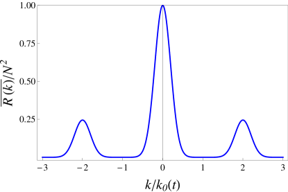
Figure 1: The average value of $R(k)$ in the large $N$ limit, for two expanding and overlapping Gaussian wave packets. The curve refers to $\alpha=5$ and $t=10\alpha$. The width $1/t$ and the distance $2\alpha/t$ among the three Gaussian functions decrease with time.

Typicality will consist in proving that this outcome is valid for the vast majority of wave functions of the condensate. In other words, in most experimental runs, each characterized by a given wave function of the condensate, one will observe an interference pattern with fringes $\sim\cos^{2}k_{0}(t)x$. Let us therefore check that the fluctuations of $R(k)$ around its average (56) are small even in the large $n$ regime. Observe that, for large times, the overlap between the functions $\mathcal{F}[\psi_{a}^{*}\psi_{b}]$, $\mathcal{F}[\psi_{b}^{*}\psi_{a}]$, and $\tilde{\rho}_{a,b}$ is very small, being $\text{O}(e^{-\alpha^{2}})$. Thus, the contributions arising from the products $\mathcal{F}[\psi_{a}^{*}\psi_{b}](k)\mathcal{F}[\psi_{b}^{*}\psi_{a}](k)$ and $\mathcal{F}[\psi_{a,b}^{*}\psi_{b,a}](k)\tilde{\rho}_{a,b}(\pm k)$ can be consistently neglected, being as small as the overlap between the two expanding Gaussian wave packets. This yields

$$(\delta R)^{2}(k,k^{\prime};t)\simeq\frac{n^{3}}{180}\left(e^{-\frac{t^{2}}{2}[k+2k_{0}(t)]^{2}}+e^{-\frac{t^{2}}{2}[k-2k_{0}(t)]^{2}}\right)\left(e^{-\frac{t^{2}}{2}[k^{\prime}+2k_{0}(t)]^{2}}+e^{-\frac{t^{2}}{2}[k^{\prime}-2k_{0}(t)]^{2}}\right)+\text{O}(N^{2}).$$ (57)

In the light of the previous observation, we can compute the $F_{i,j}$ functions in (33) and finally obtain the statistical average of quantum covariance

$$\overline{(\Delta R)^{2}}(k,k^{\prime};t)\simeq C_{3,0}(k,k^{\prime})N^{3}+C_{1,2}(k,k^{\prime})Nn^{2}+C_{0,4}(k,k^{\prime})n^{4}+C_{0,3}(k,k^{\prime})n^{3}+\text{O}(N^{2}),$$ (58)

with

$$C_{3,0}(k,k^{\prime}) = 8e^{-\frac{t^{2}}{2}(k^{2}+{k^{\prime}}^{2})}\sinh^{2}\!\left(\frac{t^{2}kk^{\prime}}{4}\right)$$ (59)

$${}-\frac{1}{4}\left(e^{-\frac{t^{2}}{2}[k+2k_{0}(t)]^{2}}+e^{-\frac{t^{2}}{2}[k-2k_{0}(t)]^{2}}\right)\left(e^{-\frac{t^{2}}{2}[k^{\prime}+2k_{0}(t)]^{2}}+e^{-\frac{t^{2}}{2}[k^{\prime}-2k_{0}(t)]^{2}}\right)$$

$${}+2e^{-\frac{t^{2}}{2}k^{2}}\left[e^{-\frac{t^{2}}{2}[k^{\prime}+2k_{0}(t)]^{2}}\sinh^{2}\!\left(\frac{t^{2}k[k^{\prime}+2k_{0}(t)]}{4}\right)+e^{-\frac{t^{2}}{2}[k^{\prime}-2k_{0}(t)]^{2}}\sinh^{2}\!\left(\frac{t^{2}k[k^{\prime}-2k_{0}(t)]}{4}\right)\right]$$

$${}+2e^{-\frac{t^{2}}{2}{k^{\prime}}^{2}}\left[e^{-\frac{t^{2}}{2}[k+2k_{0}(t)]^{2}}\sinh^{2}\!\left(\frac{t^{2}k^{\prime}[k+2k_{0}(t)]}{4}\right)+e^{-\frac{t^{2}}{2}[k-2k_{0}(t)]^{2}}\sinh^{2}\!\left(\frac{t^{2}k^{\prime}[k-2k_{0}(t)]}{4}\right)\right]$$

$${}+\frac{1}{2}e^{-\frac{t^{2}}{2}(k-k^{\prime})^{2}}\left(e^{-\frac{t^{2}}{2}[k+2k_{0}(t)][k^{\prime}+2k_{0}(t)]}+e^{-\frac{t^{2}}{2}[k-2k_{0}(t)][k^{\prime}-2k_{0}(t)]}\right)$$

$${}+\frac{1}{2}e^{-\frac{t^{2}}{2}(k+k^{\prime})^{2}}\left(e^{\frac{t^{2}}{2}[k-2k_{0}(t)][k^{\prime}+2k_{0}(t)]}+e^{\frac{t^{2}}{2}[k+2k_{0}(t)][k^{\prime}-2k_{0}(t)]}\right),$$

$$C_{1,2}(k,k^{\prime}) = \frac{1}{3}\left[8e^{-\frac{t^{2}}{2}(k^{2}+{k^{\prime}}^{2})}\sinh^{2}\!\left(\frac{t^{2}kk^{\prime}}{4}\right)-C_{3,0}(k,k^{\prime})\right],$$ (60)

$$C_{0,4}(k,k^{\prime}) = \frac{1}{180}\left(e^{-\frac{t^{2}}{2}[k+2k_{0}(t)]^{2}}+e^{-\frac{t^{2}}{2}[k-2k_{0}(t)]^{2}}\right)\left(e^{-\frac{t^{2}}{2}[k^{\prime}+2k_{0}(t)]^{2}}+e^{-\frac{t^{2}}{2}[k^{\prime}-2k_{0}(t)]^{2}}\right)=-C_{0,3}(k,k^{\prime}).$$ (61)

Also in this case, fluctuations are small when $n=\text{o}(N)$. This proves our thesis: interference is typical and occurs for the overwhelming majority of wave functions of the condensate. One can again distinguish two regimes, with threshold at $n=\text{O}(N^{3/4})$. Figure 2 displays the dominant contributions $C_{3,0}$ and $C_{0,4}$ in the two regimes.

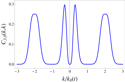
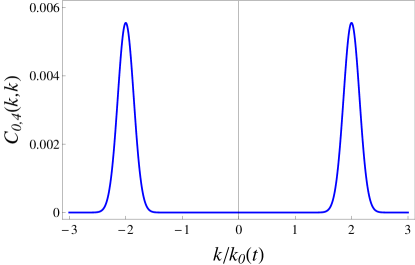
Figure 2: Dominant contributions to the variance of $R(k)$ in the asymptotic regime, when $n$ is (a) much smaller, and (b) much larger than $N^{3/4}$. Notice that the variances are in both cases peaked around $k=\pm 2k_{0}(t)$.

VI Conclusions

The search for a quantum mechanical explanation of statistical mechanics dates back to the founding fathers of quantum theory Schroedinger ; vonNeumann . In the last few years this subject has been revived and several successful new results have been obtained. For a review, see gogolin . In Refs. Lloyd ; Tasaki ; Gemmer ; Popescu1 ; Popescu2 ; Goldstein ; Sugita ; Reimann ; ref:Rigol-Nature ; Cho ; SugiuraShimizu a justification for the applicability of the canonical ensemble was given that does not rely on subjective additional randomness added by hand, or on ensemble averages. The statistical behavior is shown to be a direct consequence of a genuine quantum approach. In particular, in Refs. Lloyd ; Popescu1 ; Popescu2 it was shown that, under general assumptions on the Hamiltonian, typically random pure states of large quantum systems locally look as the microcanonical state. These works are based on typicality arguments and on the mathematical phenomenon of measure concentration Ledoux . Typicality has also been shown to be important in many emerging phenomena in physics and other sciences. An interesting application is e.g.  on the structure of entanglement and of local entropies in large quantum systems Winter ; mixmatrix ; matrix reloaded ; polarized .

In this article we have shown that typicality arguments also apply to one of the most basic quantum phenomena: interference. Two parts of a Bose-Einstein condensate, that are first separated and then let overlap, will (almost) always interfere, no matter what their wave function looks like, even if the splitting process divides the condensate in two unbalanced parts. No decoherence mechanism has been invoked. Different regimes have been identified, as a function of the scaling of $n$ with $N$. The threshold is at number fluctuations as large as $n\sim N^{\alpha}$ with $\alpha=3/4$, which for $N\simeq 5000$ atoms yields $n\simeq 600$ atoms. Interference remains observable even for such an uneven splitting process.

One of the objectives of our future research will be to analyze some recent experiments performed in Vienna Schmied ; Schmied2 ; Schmied3 ; Schmied4 ; Schmied5 ; Paraoanu that bring to light other interesting aspects of the interference of BECs, and in particular the onset to decoherence, viewed as the randomization of the relative phase as a function of the time elapsed after the splitting process.

Appendix A

In this Appendix we give closed and general forms for the $F_{i,j}$ functions appearing in (34). Let us first introduce some shorthand for the combinations of Fourier transforms that frequently appear in $F_{i,j}$:

$$I_{ab}(\bm{k}) = \tilde{\rho}_{a}(\bm{k})+\tilde{\rho}_{b}(\bm{k}),$$ (62)

$$F_{ab}(\bm{k}_{1},\bm{k}_{2}) = \mathcal{F}[\psi_{a}^{*}\psi_{b}](\bm{k}_{1})\mathcal{F}[\psi_{b}^{*}\psi_{a}](\bm{k}_{2})+\mathcal{F}[\psi_{b}^{*}\psi_{a}](\bm{k}_{1})\mathcal{F}[\psi_{a}^{*}\psi_{b}](\bm{k}_{2}),$$ (63)

$$G_{ab}(\bm{k}_{1},\bm{k}_{2}) = F_{ab}(\bm{k}_{1},\bm{k}_{2}-\bm{k}_{1})+F_{ab}(-\bm{k}_{1},\bm{k}_{2}+\bm{k}_{1}),$$ (64)

$$S_{ab}(\bm{k}_{1},\bm{k}_{2}) = \tilde{\rho}_{a}(\bm{k}_{1})\tilde{\rho}_{a}(\bm{k}_{2})+\tilde{\rho}_{b}(\bm{k}_{1})\tilde{\rho}_{b}(\bm{k}_{2}),$$ (65)

$$T_{ab}(\bm{k}_{1},\bm{k}_{2}) = \tilde{\rho}_{a}(\bm{k}_{1})\tilde{\rho}_{b}(\bm{k}_{2})+\tilde{\rho}_{b}(\bm{k}_{1})\tilde{\rho}_{a}(\bm{k}_{2}),$$ (66)

$$R_{ab}(\bm{k}) = T_{ab}(\bm{k},-\bm{k})+F_{ab}(\bm{k},-\bm{k}),$$ (67)

$$U_{ab}(\bm{k}_{1},\bm{k}_{2}) = \tilde{\rho}_{a}(\bm{k}_{1})\tilde{\rho}_{a}(\bm{k}_{2})\tilde{\rho}_{b}(\bm{k}_{1}+\bm{k}_{2})+\tilde{\rho}_{b}(\bm{k}_{1})\tilde{\rho}_{b}(\bm{k}_{2})\tilde{\rho}_{a}(\bm{k}_{1}+\bm{k}_{2}),$$ (68)

$$V_{ab}(\bm{k}_{1},\bm{k}_{2}) = \tilde{\rho}_{a}(\bm{k}_{1})\tilde{\rho}_{a}(\bm{k}_{2})\tilde{\rho}_{a}(\bm{k}_{1}+\bm{k}_{2})+\tilde{\rho}_{b}(\bm{k}_{1})\tilde{\rho}_{b}(\bm{k}_{2})\tilde{\rho}_{b}(\bm{k}_{1}+\bm{k}_{2}).$$ (69)

The functions which determine the fluctuations around the average value of $|\tilde{\rho}(\bm{k})|^{2}$ read

$$F_{4,0}(\bm{k},\bm{k}^{\prime}) = |\tilde{\rho}_{a}(\bm{k})\tilde{\rho}_{a}(\bm{k}^{\prime})|^{2}+|\tilde{\rho}_{b}(\bm{k})\tilde{\rho}_{b}(\bm{k}^{\prime})|^{2},$$ (70)

$$F_{3,1}(\bm{k},\bm{k}^{\prime}) = R_{ab}(\bm{k})S_{ab}(\bm{k}^{\prime},-\bm{k}^{\prime})+S_{ab}(\bm{k},-\bm{k})R_{ab}(\bm{k}^{\prime})+S_{ab}(\bm{k},\bm{k}^{\prime})F_{ab}(-\bm{k},-\bm{k}^{\prime})$$ (71)

$$+ S_{ab}(-\bm{k},\bm{k}^{\prime})F_{ab}(\bm{k},-\bm{k}^{\prime})+S_{ab}(\bm{k},-\bm{k}^{\prime})F_{ab}(-\bm{k},\bm{k}^{\prime})+S_{ab}(-\bm{k},-\bm{k}^{\prime})F_{ab}(\bm{k},\bm{k}^{\prime}),$$

$$F_{2,2}(\bm{k},\bm{k}^{\prime}) = |\tilde{\rho}_{a}(\bm{k})\tilde{\rho}_{b}(\bm{k}^{\prime})|^{2}+|\tilde{\rho}_{b}(\bm{k})\tilde{\rho}_{a}(\bm{k}^{\prime})|^{2}+R_{ab}(\bm{k})R_{ab}(\bm{k}^{\prime})+T_{ab}(\bm{k},\bm{k}^{\prime})F_{ab}(-\bm{k},-\bm{k}^{\prime})+T_{ab}(\bm{k},-\bm{k}^{\prime})F_{ab}(-\bm{k},\bm{k}^{\prime})$$ (72)

$$+ T_{ab}(-\bm{k},\bm{k}^{\prime})F_{ab}(\bm{k},-\bm{k}^{\prime})+T_{ab}(-\bm{k},-\bm{k}^{\prime})F_{ab}(\bm{k},\bm{k}^{\prime})+\mathcal{F}[\psi_{a}^{*}\psi_{b}](\bm{k})\mathcal{F}[\psi_{a}^{*}\psi_{b}](-\bm{k})\mathcal{F}[\psi_{b}^{*}\psi_{a}](\bm{k}^{\prime})\mathcal{F}[\psi_{b}^{*}\psi_{a}](-\bm{k}^{\prime})$$

$$+ \mathcal{F}[\psi_{b}^{*}\psi_{a}](\bm{k})\mathcal{F}[\psi_{b}^{*}\psi_{a}](-\bm{k})\mathcal{F}[\psi_{a}^{*}\psi_{b}](\bm{k}^{\prime})\mathcal{F}[\psi_{a}^{*}\psi_{b}](-\bm{k}^{\prime}),$$

$$F_{3,0}(\bm{k},\bm{k}^{\prime}) = V_{ab}(\bm{k},\bm{k}^{\prime})+V_{ab}(\bm{k},-\bm{k}^{\prime})+V_{ab}(-\bm{k},\bm{k}^{\prime})+V_{ab}(-\bm{k},-\bm{k}^{\prime}),$$ (73)

$$F_{2,1}(\bm{k},\bm{k}^{\prime}) = I_{ab}(\bm{k})G_{ab}(\bm{k}^{\prime},-\bm{k})+I_{ab}(-\bm{k})G_{ab}(\bm{k}^{\prime},\bm{k})+I_{ab}(\bm{k}^{\prime})G_{ab}(\bm{k},-\bm{k}^{\prime})+I_{ab}(-\bm{k}^{\prime})G_{ab}(\bm{k},\bm{k}^{\prime})$$ (74)

$$+ I_{ab}(\bm{k}+\bm{k}^{\prime})R_{ab}(-\bm{k},-\bm{k}^{\prime})+I_{ab}(\bm{k}-\bm{k}^{\prime})R_{ab}(\bm{k},-\bm{k}^{\prime})+I_{ab}(\bm{k}^{\prime}-\bm{k})R_{ab}(-\bm{k},\bm{k}^{\prime})+I_{ab}(-\bm{k}-\bm{k}^{\prime})R_{ab}(\bm{k},\bm{k}^{\prime})$$

$$+ U_{ab}(\bm{k},\bm{k}^{\prime})+U_{ab}(\bm{k},-\bm{k}^{\prime})+U_{ab}(-\bm{k},\bm{k}^{\prime})+U_{ab}(-\bm{k},-\bm{k}^{\prime}).$$

Notice that the $F_{i,j}$ functions with $i+j=4$ come from the eight-order term in the field operators appearing in (33), while the ones with $i+j=3$ come from the sixth-order terms under the integral in the same expression.

References

- (1) A. S. Parkins and D. F. Walls, Phys. Rep. 303, 1 (1998).
- (2) F. Dalfovo, S. Giorgini, L. P. Pitaevskii, and S. Stringari, Rev. Mod. Phys. 71, 463 (1999).
- (3) A. J. Leggett, Rev. Mod. Phys. 73, 307 (2001).
- (4) I. Bloch, J. Dalibard, and W. Zwerger, Rev. Mod. Phys. 80, 885 (2008).
- (5) L. Pitaevskii and S. Stringari, Bose-Einstein Condensation (Oxford University Press, Oxford, 2003).
- (6) C. J. Pethick and H. Smith, Bose-Einstein Condensation in Dilute Gases, 2nd ed. (Cambridge University Press, Cambridge, 2008).
- (7) A. J. Leggett, Quantum Liquids: Bose Condensation and Cooper Pairing in Condensed-Matter Systems (Oxford University Press, Oxford, 2006).
- (8) M. R. Andrews, C. G. Townsend, H.-J. Miesner, D. S. Durfee, D. M. Kurn, and W. Ketterle, Science 275, 637 (1997).
- (9) R. Hanbury Brown and R. Q. Twiss, Nature (London) 177, 27 (1956).
- (10) R. Hanbury Brown and R. Q. Twiss, Nature (London) 178, 1046 (1956).
- (11) R. Feynman, R. Leighton, and M. Sand, The Feynman Lectures on Physics (Addison Wesley Longman, Reading, MA, 1970), Vol. 3.
- (12) R. Loudon, The Quantum Theory of Light (Oxford University Press, Oxford, 2000).
- (13) L. Mandel and E. Wolf, Optical Coherence and Quantum Optics (Cambridge University Press, Cambridge, 1995).
- (14) J. Javanainen and S. M. Yoo, Phys. Rev. Lett. 76, 161 (1996).
- (15) J. I. Cirac, C. W. Gardiner, M. Naraschewski, and P. Zoller, Phys. Rev. A 54, 3714(R) (1996).
- (16) T. Wong, M. J. Collett, and D. F. Walls, Phys. Rev. A 54, 3718(R) (1996).
- (17) Y. Castin and J. Dalibard, Phys. Rev. A 55, 4330 (1997).
- (18) A. J. Leggett and F. Sols, Found. Phys. 21, 353 (1991).
- (19) E. Altman, E. Demler, and M. D. Lukin, Phys. Rev. A 70, 013603 (2004).
- (20) A. Polkovnikov, E. Altman, and E. Demler, Proc. Natl. Acad. Sci. USA 103, 6125 (2006).
- (21) V. Gritsev, E. Altman, E. Demler, and A. Polkovnikov, Nature Phys. 2, 705 (2006).
- (22) A. Polkovnikov, Europhys. Lett. 78, 10006 (2007).
- (23) A. Imambekov, V. Gritsev, and E. Demler, in Ultra-Cold Fermi Gases, Vol. 164 of International School of Physics “Enrico Fermi”, edited by M. Inguscio, W. Ketterle, and C. Salomon (IOS, Amsterdam, 2007), pp. 535–606.
- (24) V. Gritsev, E. Demler, and A. Polkovnikov, Phys. Rev. A 78, 063624 (2008).
- (25) Z. Hadzibabic, S. Stock, B. Battelier, V. Bretin, and J. Dalibard, Phys. Rev. Lett. 93, 180403 (2004).
- (26) S. Stock, Z. Hadzibabic, B. Battelier, M. Cheneau, and J. Dalibard, Phys. Rev. Lett. 95, 190403 (2005).
- (27) Z. Hadzibabic, P. Krüger, M. Cheneau, B. Battelier, and J. Dalibard, Nature (London) 441, 1118 (2006).
- (28) P. Krüger, Z. Hadzibabic, and J. Dalibard, Phys. Rev. Lett. 99, 040402 (2007).
- (29) K. Góral, M. Gajda, and K. Rza̧żewski, Phys. Rev. A 66, 051602 (R) (2002).
- (30) T. Schumm, S. Hofferberth, L. M. Andersson, S. Wildermuth, S. Groth, I. Bar-Joseph, J. Schmiedmayer, and P. Krüger, Nature Phys. 1, 57 (2005).
- (31) S. Hofferberth, I. Lesanovsky, B. Fischer, J. Verdu, and J. Schmiedmayer, Nature Phys. 2, 710 (2006).
- (32) S. Hofferberth, I. Lesanovsky, B. Fischer, T. Schumm, and J. Schmiedmayer, Nature (London) 449, 324 (2007).
- (33) S. Hofferberth, I. Lesanovsky, T. Schumm, A. Imambekov, V. Gritsev, E. Demler, and J. Schmiedmayer, Nature Phys. 4, 489 (2008).
- (34) T. Langen, R. Geiger, M. Kuhnert, B. Rauer, and J. Schmiedmayer, Nature Phys. 9, 640 (2013).
- (35) G. S. Paraoanu, J. Low. Temp. Phys. 153, 285 (2008); Phys. Rev. A 77, 041605 (R) (2008).
- (36) M. Iazzi and K. Yuasa, Phys. Rev. A 83, 033611 (2011).
- (37) K. Maussang, G. E. Marti, T. Schneider, P. Treutlein, Y. Li, A. Sinatra, R. Long, J. Estève, and J. Reichel, Phys. Rev. Lett. 105, 080403 (2010).
- (38) P. Facchi, G. Florio, U. Marzolino, G. Parisi, and S. Pascazio, J. Phys. A: Math. Theor. 43, 225303 (2010).
- (39) S. Ando, K. Yuasa, and M. Iazzi, Int. J. Quant. Inf. 9, 431 (2011).
- (40) E. Schroedinger, Statistical Thermodynamics (Dover Publications, New York 1989).
- (41) J. von Neumann, Mathematical Foundation of Quantum Mechanics (Princeton University Press, Princeton 1955).
- (42) C. Gogolin, Pure State Quantum Statistical Mechanics, Master Thesis, University of Würzburg, arXiv:1003.5058 [quant-ph] (2010).
- (43) S. Lloyd, Black Holes, Demons and the Loss of Coherence: How Complex Systems Get Information, and What They Do with It, PhD thesis, Rockefeller University (1991).
- (44) H. Tasaki, Phys. Rev. Lett. 80, 1373 (1998).
- (45) J. Gemmer and G. Mahler, Eur. Phys. J. B 31, 249 (2003).
- (46) S. Popescu, A. J. Short, and A. Winter, The foundations of Statistical Mechanics from Entanglement: Individual States vs. Averages, quant-ph/0511225 (2005).
- (47) S. Popescu, A. J. Short, and A. Winter, Nature Phys. 2, 754 (2006).
- (48) S. Goldstein, J. L. Lebowitz, R. Tumulka, and N. Zanghì, Phys. Rev. Lett. 96, 050403 (2006).
- (49) A. Sugita, Nonlinear Phenom. Complex Syst. 10, 192 (2007) [cond-mat/0602625 (2006)].
- (50) P. Reimann, Phys. Rev. Lett. 99, 160404 (2007); 101, 190403 (2008).
- (51) M. Rigol, V. Dunjko, and M. Olshanii, Nature (London) 452, 854 (2008).
- (52) J. Cho and M. S. Kim, arXiv:0911.2110 (2009).
- (53) S. Sugiura and A. Shimizu, Phys. Rev. Lett. 108, 240401 (2012); 111, 010401 (2013).
- (54) M. Ledoux, The Concentration of Measure Phenomenon, vol. 89 of Mathematical Surveys and Monographs (American Mathematical Society, 2001).
- (55) P. Hayden, D.W. Leung, and A. Winter, Commun. Math. Phys. 265, 95 (2006).
- (56) A. De Pasquale, P. Facchi, V. Giovannetti, G. Parisi, S. Pascazio, and A. Scardicchio, J. Phys. A: Math. Theor. 45, 015308 (2012).
- (57) P. Facchi, G. Florio, G. Parisi, S. Pascazio, and K. Yuasa, Phys. Rev. A 87, 052324 (2013).
- (58) F. D. Cunden, P. Facchi, and G. Florio, J. Phys. A: Math. Theor. 46, 315306 (2013).