Observational constraints on slow-roll inflation coupled to a Gauss-Bonnet term

Abstract

We study slow-roll inflation with a Gauss-Bonnet term that is coupled to an inflaton field nonminimally. We investigate the inflationary solutions for a specific type of the nonminimal coupling to the Gauss-Bonnet term and inflaton potential both analytically and numerically. We also calculate the observable quantities such as the power spectra of the scalar and tensor modes, the spectral indices, the tensor-to-scalar ratio and the running spectral indices. Finally, we constrain our result with the observational data by Planck and BICEP2 experiment.

I Introduction

Recent experiments and observations including Planck Ade:2013zuv , LHC Chatrchyan:2012ufa , and BICEP2 Ade:2014xna confirmed that the inflation paradigm is believed to be successful for explaining the evolution of our Universe and generation of large scale structure formation. The cosmic microwave background (CMB) observations by Planck and WMAP imply that our Universe is Gaussian, adiabatic, and nearly scale invariant. Although there are some debates Ijjas:2013vea , the Planck data seem to favor the inflationary model with the simple scalar field potential, especially the convex-type potential Ade:2013uln . But recent BICEP2 combined with Planck data seems to favor the concave-type potential, especially the $\phi^{2}$ potential.

While Planck and WMAP provide the upper bound on the tensor-to-scalar ratio ($r<0.12$), recent BICEP2 telescope Ade:2014xna at the South Pole reported the detection of B-mode polarization signal Michael:2014 ,Raphael:2014 which is generated by the tensor perturbation (gravitational wave modes) in an inflationary period. According to BICEP2, $r=0.20$ at $5.2\sigma$ with $r=0$ disfavored at $7.0\sigma$. This tensor-to-scalar ratio value is larger than the upper bound by Planck + WMAP. It has been widely studied how to reconcile this discrepancy between two data, and one simple resolution, which was suggested in Ref. Ade:2014xna , is to consider the running spectral index, $dn_{s}/d\ln k$.

Although inflation is believed to solve a lot of the outstanding problems of the standard big bang cosmology such as the horizon and flatness problem, there are still several unsolved problems in an inflation scenario, for example, the flat potential problem, initial singularity problem, and quantum gravity (trans-Planckian problem).

Especially, if we think over the very early Universe approaching the Planck scale, we could consider Einstein gravity with some corrections as the effective theory of the ultimate quantum gravity. For instance, the higher derivative terms of gravity with nontrivial gravitational self-interactions naturally appear in the low energy limits of string theories. The presence of curvature squared terms such as a Gauss-Bonnet (GB) combination does not have any ghost particles as well as any problem with the unitarity. Additionally, the order of the gravitational equation of motion, the second-order derivatives of the metric tensor, does not change if there is no nonminimal coupling to a Gauss-Bonnet term Callan:1985ia . Fortunately, the theory with a nonminimally coupled Gauss-Bonnet term could provide the possibility of avoiding the initial singularity of the Universe Antoniadis:1992rq . It may violate the energy condition thanks to the presence of the term in the singularity theorem Hawking:1969sw . In this perspective, one could introduce the Einstein theory of gravity having a scalar field with a nonminimally coupled Gauss-Bonnet term as the effective theory added a quantum correction.

Generally, the Gauss-Bonnet term in four dimensions is known as the topological term, so the dynamics is not influenced by the Gauss-Bonnet term. In order to consider the effect of the Gauss-Bonnet term on the spacetime as well as the field evolution, the Gauss-Bonnet term is required to be coupled to the matter field. Recently a number of papers with this motivation were studied Hwang:2000 ,Kawai:1999 and discussed phenomenology in detail in Satoh:2008 ,Satoh:2008a ,Satoh:2010 ,Guo:2010jr and Jiang:2013gza . In Refs. Guo:2010jr ,Jiang:2013gza , the authors studied the specific inflationary model with the Gauss-Bonnet term constrained by the WMAP data in Guo:2010jr and by the Planck data in Jiang:2013gza . They analytically derived the power spectra of the scalar and tensor perturbations. They employed a monomial potential and an inverse monomial Gauss-Bonnet coupling that satisfies $V(\phi)\xi(\phi)\sim\text{const}$. These choices of the potential and Gauss-Bonnet coupling provide the relatively large parameter values, $\alpha\equiv 4\kappa^{4}V_{0}\xi_{0}/3\sim\mathcal{O}(10^{-2})$, to be consistent with observations and showed that a positive (or negative) coupling leads to a reduction (or enhancement) of the tensor-to-scalar ratio.

In this work, we try to relax the condition $V(\phi)\xi(\phi)\sim\text{const}$ and then constrain from the recent observations by Planck and BICEP2. We also calculate the spectral indices of the scalar and tensor perturbations, the tensor-to-scalar ratio and the running spectral index.

The outline of this paper is as follows: In Sec. II, we set up the basic framework with the Gauss-Bonnet term for this work. The $e$-folding numbers are calculated and then give a constraint on the model parameter. In Sec. III, we briefly review the linear perturbations with the Gauss-Bonnet coupling term and then calculate the observable quantities such as the power spectra, the spectral indices, the tensor-to-scalar ratio and the running spectral indices. In Sec. IV, we examine the specific models consistent with our motivations. We compare our result with the observational data by the Planck data and recent BICEP2. Finally, we summarize our results in Sec. V.

II Slow-roll inflation with the GB term

We consider an action with the Gauss-Bonnet term that is coupled to a scalar field

$$S= \int_{\mathcal{M}}d^{4}x\sqrt{-g}\left[\frac{1}{2\kappa^{2}}R-\frac{1}{2}g^{\mu\nu}\partial_{\mu}\phi\partial_{\nu}\phi-V(\phi)-\frac{1}{2}\xi(\phi)R_{\rm GB}^{2}\right],$$ (1)

where $\phi$ is an inflaton field with a potential $V(\phi)$, $R$ is the Ricci scalar curvature of the spacetime $\mathcal{M}$, $R^{2}_{\rm GB}=R_{\mu\nu\rho\sigma}R^{\mu\nu\rho\sigma}-4R_{\mu\nu}R^{\mu\nu}+R^{2}$ is the Gauss-Bonnet term, and $\kappa^{2}=8\pi G$. The Gauss-Bonnet coupling $\xi(\phi)$ is required to be a function of a scalar field in order to give nontrivial effects on the background dynamics.

Varying the action (1) with respect to $g_{\mu\nu}$ and $\phi$ yields the Einstein and field equation

$$R_{\mu\nu}-\frac{1}{2}g_{\mu\nu}R=\kappa^{2}\left(\partial_{\mu}\phi\partial_{\nu}\phi-\frac{1}{2}g_{\mu\nu}(g^{\rho\sigma}\partial_{\rho}\phi\partial_{\sigma}\phi+2V)+T_{\mu\nu}^{GB}\right),$$ (2)

$$\square\phi-V_{\phi}-\frac{1}{2}T^{GB}=0,$$ (3)

where $\square\equiv\partial_{\mu}\partial^{\mu}$. $T_{\mu\nu}^{GB}$ and $T^{GB}$ are the energy-momentum tensor and its trace for the Gauss-Bonnet term, respectively, which are given by

$$T_{\mu\nu}^{GB}= 4(\partial^{\rho}\partial^{\sigma}\xi R_{\mu\rho\nu\sigma}-\square\xi R_{\mu\nu}+2\partial_{\rho}\partial_{(\mu}\xi{R^{\rho}}_{\nu)}-\frac{1}{2}\partial_{\mu}\partial_{\nu}\xi R)$$

$$-2(2\partial_{\rho}\partial_{\sigma}\xi R^{\rho\sigma}-\square\xi R)g_{\mu\nu},$$ (4)

$$T^{GB}= \xi_{\phi}R_{GB}^{2}.$$ (5)

In a spatially flat Friedmann-Robertson-Walker universe with a scale factor $a$,

$$ds^{2}=-dt^{2}+a(t)^{2}\delta_{ij}dx^{i}dx^{j},$$ (6)

the background Einstein and field equations yield

$$H^{2}=\frac{\kappa^{2}}{3}\left(\frac{1}{2}\dot{\phi}^{2}+V+12\dot{\xi}H^{3}\right),$$ (7)

$$\dot{H}=-\frac{\kappa^{2}}{2}\left(\dot{\phi}^{2}-4\ddot{\xi}H^{2}-4\dot{\xi}H(2\dot{H}-H^{2})\right),$$ (8)

$$\ddot{\phi}+3H\dot{\phi}+V_{,\phi}+12\xi_{,\phi}H^{2}\left(\dot{H}+H^{2}\right)=0,$$ (9)

where a dot represents a derivative with respect to the cosmic time $t$, $H\equiv\dot{a}/a$ denotes the Hubble parameter, and $V_{,\phi}=\partial V/\partial\phi,\,\,\xi_{,\phi}=\partial\xi/\partial\phi$. Since $\xi$ is a function of $\phi$, $\dot{\xi}$ implies $\dot{\xi}=\xi_{,\phi}\dot{\phi}$. If $\xi$ is a constant, then Eqs. (7)–(9) are reduced to those for standard inflation without the Gauss-Bonnet coupling.

In this work, we consider slow-roll inflation with the inflaton potential and Gauss-Bonnet coupling satisfying the slow-roll approximations

$$\dot{\phi}^{2}/2\ll V,\quad\ddot{\phi}\ll 3H\dot{\phi},\quad 4\dot{\xi}H\ll 1,\quad\ddot{\xi}\ll\dot{\xi}H.$$ (10)

In addition to the usual slow-roll approximations, we introduce two more conditions related to the Gauss-Bonnet coupling.

To reflect these approximations, we introduce the slow-roll parameters,

$$\epsilon =-\frac{\dot{H}}{H^{2}},\quad\eta=\frac{\ddot{H}}{H\dot{H}},\quad\zeta=\frac{\dddot{H}}{H^{2}\dot{H}},$$

$$\delta_{1} =4\kappa^{2}\dot{\xi}H,\quad\delta_{2}=\frac{\ddot{\xi}}{\dot{\xi}H},\quad\delta_{3}=\frac{\dddot{\xi}}{\dot{\xi}H^{2}}.$$ (11)

We have checked the validity of the new slow-roll parameters during an accelerating phase numerically in Fig. 1.

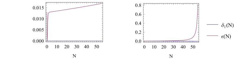
Figure 1: Left: evolution of the slow-roll parameters $\epsilon$ and $\delta_{1}$ for $\xi(\phi)=\xi_{0}e^{-\lambda\phi}$ with $\lambda=-0.1$.   Right: evolution of the slow-roll parameters $\epsilon$ and $\delta_{1}$ for $\xi(\phi)=\xi_{0}\phi^{2}$.

If the slow-roll approximations (10) are taken into account, the background equations, (7)-(9), reduce to

$$H^{2}\simeq\frac{\kappa^{2}}{3}V,$$ (12)

$$\dot{H}\simeq-\frac{\kappa^{2}}{2}(\dot{\phi}^{2}+4\dot{\xi}H^{3}),$$ (13)

$$3H\dot{\phi}+V_{,\phi}+12\xi_{,\phi}H^{4}\simeq 0,$$ (14)

which allows us to obtain the number of $e$-folds

$$N(\phi)=\int_{t}^{t_{e}}Hdt\simeq\int_{\phi_{e}}^{\phi}\frac{3\kappa^{2}V}{3V_{,\phi}+4\kappa^{4}\xi_{,\phi}V^{2}}d\phi\equiv\int^{\phi}_{\phi_{e}}\frac{\kappa^{2}}{Q}d\phi.$$ (15)

where a $\phi_{e}$ is determined from the condition $\epsilon(\phi_{e})=1$ and

$$Q\equiv\frac{V_{,\phi}}{V}+\frac{4}{3}\kappa^{4}\xi_{,\phi}V.$$ (16)

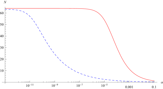
Figure 2: $e$-folding numbers with $\alpha\equiv\frac{4}{3}\kappa^{4}V_{0}\xi_{0}$ for $V=V_{0}\phi^{2},\,\,\xi=\xi_{0}\phi^{2}$ (solid line) and $V=V_{0}\phi^{4},\,\,\xi=\xi_{0}\phi^{4}$ (dashed line).

If we choose $V=V_{0}\phi^{n}$ and $\xi=\xi_{0}\phi^{n}$, the number of $e$-folds are calculated assuming $\phi_{e}$ is negligible compared to $\phi_{i}$ as

$$N=\int^{\phi_{i}}_{\phi_{e}}\frac{\kappa^{2}}{Q}\simeq\frac{\kappa^{2}\phi_{i}^{2}}{2n}{}_{2}F_{1}\left(1,\frac{1}{n},1+\frac{1}{n};-\alpha\phi_{i}^{2n}\right),$$ (17)

where ${}_{2}F_{1}$ is the hypergeometric function and $\alpha\equiv\frac{4}{3}\kappa^{4}V_{0}\xi_{0}$. We plot the number of $e$-folds $N$ with $\alpha$ for $n=2$ (solid line) and $n=4$ (dashed line) in Fig. 2. The condition of $N\gtrsim 60$ requires $\alpha\lesssim\alpha_{c}=10^{-6}\,\,M_{p}^{-4}$ for $n=2$ and $\alpha\lesssim\alpha_{c}=10^{-12}\,\,M_{p}^{-8}$ for $n=4$. Here, $\alpha_{c}$ is the value when $\alpha$ becomes nearly constant. We find that $N$ approaches $N_{max}$ as $\alpha$ decreases to $\alpha_{c}$. Because the hypergeometric function ${}_{2}F_{1}$ is constant for $\alpha\lesssim\alpha_{c}$, $N$ cannot become larger than $N_{max}$ unless $\phi_{i}$ increases. $\phi_{i}=15M_{p}\,\,(n=2)$ and $\phi_{i}=22M_{p}\,\,(n=4)$ are required to obtain $N\simeq 60$ in Fig. 2.

It is convenient to express the slow-roll parameters (11) in terms of the potential and Gauss-Bonnet coupling:

$$\epsilon= \frac{1}{2\kappa^{2}}\frac{V_{\phi}}{V}Q,$$ (18)

$$\eta= -\frac{V_{\phi\phi}Q}{\kappa^{2}V_{\phi}}-\frac{1}{\kappa^{2}}Q_{\phi},$$ (19)

$$\zeta= \frac{V_{\phi\phi\phi}Q^{2}}{\kappa^{4}V_{\phi}}+\frac{V_{\phi\phi}Q^{2}}{2\kappa^{4}V}+\frac{3V_{\phi\phi}Q_{\phi}Q}{\kappa^{4}V_{\phi}}+\frac{V_{\phi}Q_{\phi}Q}{2\kappa^{4}V}$$

$$+\frac{1}{\kappa^{4}}Q_{\phi}^{2}+\frac{1}{\kappa^{4}}Q_{\phi\phi}Q,$$ (20)

$$\delta_{1}= -\frac{4\kappa^{2}}{3}\xi_{\phi}VQ,$$ (21)

$$\delta_{2}= -\frac{\xi_{\phi\phi}Q}{\kappa^{2}\xi_{\phi}}-\frac{V_{\phi}Q}{2\kappa^{2}V}-\frac{1}{\kappa^{2}}Q_{\phi},$$ (22)

$$\delta_{3}= \frac{\xi_{\phi\phi\phi}Q^{2}}{\kappa^{4}\xi_{\phi}}+\frac{3\xi_{\phi\phi}V_{\phi}Q2}{2\kappa^{4}\xi_{\phi}V}+\frac{3\xi_{\phi\phi}Q_{\phi}Q}{\kappa^{4}\xi_{\phi}}+\frac{V_{\phi\phi}Q^{2}}{2\kappa^{4}V}$$

$$+\frac{2V_{\phi}Q_{\phi}Q}{\kappa^{4}V}+\frac{1}{\kappa^{4}}Q_{\phi}^{2}+\frac{1}{\kappa^{4}}QQ_{\phi\phi}.$$ (23)

Equation (14) becomes for $V=V_{0}\phi^{2}$ and $\xi=\xi_{0}\phi^{2}$

$$\dot{\phi}\approx-\sqrt{\frac{\alpha}{\xi_{0}\kappa^{6}}}(1+\alpha\phi^{4}),$$ (24)

and then we get the solution assuming $\alpha$-term is negligibly small from Fig. 2,

$$\phi(t)\sim-\sqrt{\frac{\alpha}{\xi_{0}\kappa^{6}}}t+\text{const}.$$ (25)

We find that this slow-roll trajectory is the attractor solution in Fig. 3. The slow-roll trajectories of Eqs.(12)–(14) were proved to be the attractor solutions generally when the Gauss-Bonnet term is coupled to the scalar field in Ref. Guo:2010jr . We compare the attractor behavior for three cases: standard chaotic inflation (upper), chaotic inflation with the monomial Gauss-Bonnet coupling (middle), and chaotic inflation with the inverse monomial Gauss-Bonnet coupling (below) (which was considered in Ref. Guo:2010jr ) in Fig. 3.

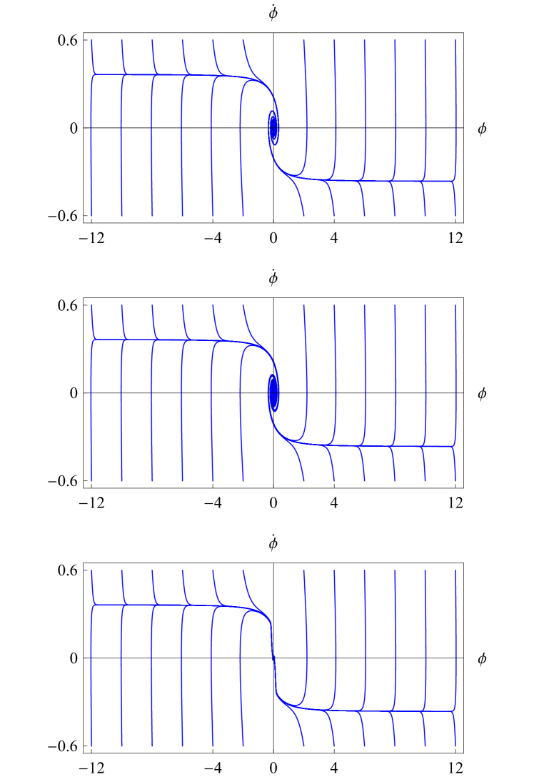
Figure 3: Attractor-type solutions of the background equations of motion for standard inflation without the Gauss-Bonnet term, chaotic inflation with the monomial Gauss-Bonnet coupling, and chaotic inflation with the inverse monomial Gauss-Bonnet coupling

III Linear Perturbations and Power Spectra

We briefly review the linear perturbations with the Gauss-Bonnet coupling in this section.

The linearized metric in the comoving gauge in which $\delta\phi=0$ takes the form

$$ds^{2}=a(\tau)^{2}[-d\tau^{2}+\{(1-2\mathcal{R})\delta_{ij}+h_{ij}\}dx^{i}dx^{j}],$$ (26)

where $\mathcal{R}$ represents the curvature perturbation on the uniform field hypersurfaces and $h_{ij}$ is the tensor perturbation that satisfies $h_{i}^{i}=0={h^{i}}_{j,i}$.

If we perform the Fourier transform of $\mathcal{R}$ and $h_{ij}$,

$$\mathcal{R}(\tau,{\bf x})= \frac{1}{z_{s}}\int\frac{d^{3}k}{(2\pi)^{3/2}}{v}_{s}(\tau,k)e^{i{\bf k}\cdot{\bf x}},$$ (27)

$$h_{ij}(\tau,{\bf x})= \frac{2}{z_{t}}\sum_{\lambda}\int\frac{d^{3}k}{(2\pi)^{3/2}}v^{\lambda}_{t}(\tau,k)\epsilon_{\lambda,ij}e^{i{\bf k}\cdot{\bf x}},$$ (28)

where $\epsilon_{ij}$ is a polarization tensor, Sasaki-Mukhanov equations for $v_{s}$ and $v_{t}$ are derived from linearizing Eqs. (2)–(3)

$$v_{s}^{\prime\prime}+\left(c_{s}^{2}k^{2}-\frac{z^{\prime\prime}_{s}}{z_{s}}\right)v_{s}=0,$$ (29)

$$v_{t}^{\prime\prime}+\left(c_{t}^{2}k^{2}-\frac{z_{t}^{\prime\prime}}{z_{t}}\right)v_{t}=0,$$ (30)

where Guo:2010jr Hwang:2005hb

$$z_{s} \equiv\sqrt{\frac{a^{2}(\dot{\phi}^{2}+6\dot{\xi}H^{3}\Delta)}{H^{2}(1-\frac{1}{2}\Delta)^{2}}},\quad\Delta=\frac{4\kappa^{2}\dot{\xi}H}{1-4\kappa^{2}\dot{\xi}H},$$ (31)

$$z_{t} \equiv\sqrt{\frac{a^{2}}{\kappa^{2}}(1-4\kappa^{2}\dot{\xi}H)},$$ (32)

and

$$c_{s}^{2}\equiv 1+\frac{2(\dot{H}-\kappa^{2}\dot{\xi}H(H^{2}+4\dot{H})+\kappa^{2}\ddot{\xi}H^{2})\Delta^{2}}{\kappa^{2}\dot{\phi}^{2}+6\kappa^{2}\dot{\xi}H^{3}\Delta},$$ (33)

$$c_{t}^{2}\equiv 1-\frac{4\kappa^{2}(\ddot{\xi}-\dot{\xi}H)}{1-4\kappa^{2}\dot{\xi}H}.$$ (34)

Here, a prime represents a derivative with respect to the conformal time $\tau=\int a^{-1}dt$.

$z_{A}$ and $c_{A}^{2}$, where $A=\{s,t\}$, can be written in terms of the slow-roll parameters Guo:2010jr Hwang:2005hb using the definitions of the slow-roll parameters (11):

$$z_{s}= \sqrt{\frac{a^{2}}{\kappa^{2}}\frac{2\epsilon-\delta_{1}(1+2\epsilon-\delta_{2})+\frac{3}{2}\delta_{1}\Delta}{(1-\frac{1}{2}\Delta)^{2}}},\quad\Delta=\frac{\delta_{1}}{1-\delta_{1}},$$ (35)

$$z_{t}= \sqrt{\frac{a^{2}}{\kappa^{2}}(1-\delta_{1})},$$ (36)

$$c_{s}^{2}= 1-\frac{(4\epsilon+\delta_{1}(1-4\epsilon-\delta_{2}))\Delta^{2}}{4\epsilon-2\delta_{1}-2\delta_{1}(2\epsilon-\delta_{2})+3\delta_{1}\Delta},$$ (37)

$$c_{t}^{2}= 1+\frac{\delta_{1}(1-\delta_{2})}{1-\delta_{1}},$$ (38)

where we have used the following relation from Eqs. (7)–(8):

$$\frac{\kappa^{2}\dot{\phi}^{2}}{H^{2}}=2\epsilon-\delta_{1}(1+2\epsilon-\delta_{2}).$$ (39)

If one keeps the leading order of the slow-roll parameters in $z_{A}^{\prime\prime}/z_{A}$ using (35)–(36), Eqs. (29)–(30) become

$$v_{A}^{\prime\prime}+\left(c_{A}^{2}k^{2}-\frac{\nu_{A}^{2}-1/4}{\tau^{2}}\right)v_{A}=0,$$ (40)

where the parameters are given by up to leading order in slow-roll parameters

$$\nu_{s} \simeq\frac{3}{2}+\epsilon+\frac{2\epsilon(2\epsilon+\eta)-\delta_{1}(\delta_{2}-\epsilon)}{4\epsilon-2\delta_{1}}$$ (41)

$$\nu_{t} \simeq\frac{3}{2}+\epsilon.$$ (42)

In deriving (40), we use the following relation:

$$\tau =-\frac{1}{aH}\frac{1}{1-\epsilon}.$$ (43)

One can obtain the exact solutions for (40) assuming that the slow-roll parameters are constants,

$$v_{A} =\frac{\sqrt{\pi|\tau|}}{2}[c^{A}_{1}(k)H_{\nu_{A}}^{(1)}(c_{A}k|\tau|)+c^{A}_{2}(k)H_{\nu_{A}}^{(2)}(c_{A}k|\tau|)],$$ (44)

where $H_{\nu}^{(i)}\,\,(i=1,2)$ are the first and second kind Hankel functions. $c^{A}_{i}\,\,(i=1,2)$ are the coefficients that are determined from the initial conditions and satisfy the normalization conditions

$$|c^{A}_{2}|^{2}-|c^{A}_{1}|^{2}=1.$$ (45)

If we adopt the Bunch-Davies vacuum for the initial fluctuation modes at $c_{A}k|\tau|\gg 1$ by taking the positive mode frequency, the initial modes are given by

$$v_{A}=\frac{1}{\sqrt{2c_{A}k}}e^{ic_{A}k|\tau|}.$$ (46)

These modes correspond to the choice of the coefficients

$$c_{1}^{A}=e^{i(\nu_{A}+\frac{1}{2})\frac{\pi}{2}},\quad c_{2}^{A}=0,$$ (47)

where we have used the asymptotic form of the Hankel functions in the limit $x\equiv c_{A}k|\tau|\gg 1$,

$$H_{\nu_{A}}^{(1,2)}(x)\sim\sqrt{\frac{2}{\pi x}}e^{\pm i(x-(\nu_{A}+\frac{1}{2})\frac{\pi}{2})}.$$ (48)

Then the exact solution (44) becomes

$$v_{A}=\frac{\sqrt{\pi|\tau|}}{2}e^{i(\nu_{A}+\frac{1}{2})\frac{\pi}{2}}H_{\nu_{A}}^{(1)}(c_{A}k|\tau|).$$ (49)

The power spectra of the scalar and tensor modes are calculated with (49) on the large scales. Since the first kind Hankel function is approximated in the large scale limit ($c_{A}k|\tau|\ll 1$) as

$$H_{\nu_{A}}^{(1)}\sim\frac{2}{1-e^{2i\nu_{A}\pi}}\biggl{\{}\frac{1}{\Gamma(1+\nu_{A})}\left(\frac{x}{2}\right)^{\nu_{A}}-\frac{e^{i\nu_{A}\pi}}{\Gamma(1-\nu_{A})}\left(\frac{x}{2}\right)^{-\nu_{A}}\biggr{\}},$$ (50)

where the second term is dominant, one can obtain the power spectra for the scalar and tensor modes on the large scales

$$\mathcal{P}_{s} =\frac{k^{3}}{2\pi^{2}}\left|\frac{v_{s}}{z_{s}}\right|^{2}$$

$$\simeq\frac{\csc^{2}\nu_{s}\pi}{\pi\mathcal{D}_{s}^{2}\Gamma^{2}(1-\nu_{s})}\frac{1}{c_{s}^{3}|\tau|^{2}a^{2}}\biggl{(}\frac{c_{s}k|\tau|}{2}\biggr{)}^{3-2\nu_{s}},$$ (51)

$$\mathcal{P}_{t} =2\frac{k^{3}}{2\pi^{2}}\left|\frac{2v_{t}}{z_{t}}\right|^{2}$$

$$\simeq 8\frac{\csc^{2}\nu_{t}\pi}{\pi\mathcal{D}_{t}^{2}\Gamma^{2}(1-\nu_{t})}\frac{1}{c_{t}^{3}|\tau|^{2}a^{2}}\biggl{(}\frac{c_{t}k|\tau|}{2}\biggr{)}^{3-2\nu_{t}},$$ (52)

where the factor 2 of the tensor power spectrum comes from the two polarization states and we define

$$z_{A} \equiv\mathcal{D}_{A}a^{2},$$

$$\mathcal{D}_{s}^{2} =\frac{2\epsilon-\delta_{1}(1+2\epsilon-\delta_{2})+\frac{3}{2}\delta_{1}\Delta}{\kappa^{2}(1-\frac{1}{2}\Delta)^{2}},$$

$$\mathcal{D}_{t}^{2} =\frac{1-\delta_{1}}{\kappa^{2}}.$$

The spectral indices of the scalar and tensor modes and the tensor-to-scalar ratio are given by

$$n_{s}-1 \equiv\frac{d\ln\mathcal{P}_{s}}{d\ln k}$$

$$=3-2\nu_{s}\approx-2\epsilon-\frac{2\epsilon(2\epsilon+\eta)-\delta_{1}(\delta_{2}-\epsilon)}{2\epsilon-\delta_{1}},$$ (53)

$$n_{t} \equiv\frac{d\ln\mathcal{P}_{t}}{d\ln k}=3-2\nu_{t}\approx-2\epsilon,$$ (54)

$$r \equiv\frac{\mathcal{P}_{t}}{\mathcal{P}_{s}}\approx 8(2\epsilon-\delta_{1}).$$ (55)

We can also calculate the running spectral indices of the scalar and tensor modes

$$\frac{dn_{s}}{d\ln k}\approx -2\epsilon(2\epsilon+\eta)+\frac{(2\epsilon(2\epsilon+\eta)-\delta_{1}(\delta_{2}-\epsilon))^{2}}{(2\epsilon-\delta_{1})^{2}}$$

$$-\frac{2\epsilon(8\epsilon^{2}+7\epsilon\eta+\zeta)+\delta_{1}(\epsilon^{2}+\epsilon\eta+\epsilon\delta_{2}-\delta_{3})}{2\epsilon-\delta_{1}}$$ (56)

$$\frac{dn_{t}}{d\ln k}\approx -2(2\epsilon^{2}+\epsilon\eta).$$ (57)

where we have used from (11)

$$\frac{d\epsilon}{d\ln k} =2\epsilon^{2}+\epsilon\eta,$$ (58)

$$\frac{d\eta}{d\ln k} =\epsilon\eta-\eta^{2}+\zeta,$$ (59)

$$\frac{d\delta_{1}}{d\ln k} =\delta_{1}(\delta_{2}-\epsilon),$$ (60)

$$\frac{d\delta_{2}}{d\ln k} =\epsilon\delta_{2}-\delta_{2}^{2}+\delta_{3}.$$ (61)

IV Models

In this section, we calculate the $n_{s},\,\,n_{t},\,\,r$, and $\frac{dn_{s}}{d\ln k}$ for the specific models using Eqs. (III)–(56) and then constrain our model predictions with the recent CMB observational data from Planck and BICEP2.

IV.1 Exponential potential with an exponential Gauss-Bonnet coupling

Let us start with the exponential potential and exponential coupling to the GB term

$$V(\phi)=V_{0}e^{-\lambda\phi},\quad\xi(\phi)=\xi_{0}e^{-\lambda\phi},$$ (62)

where $V_{0},\xi_{0}$ and $\lambda$ are constants. One can calculate the slow-roll parameters, (18)–(II), for the model given by (62)

$$\epsilon = \frac{1}{2}\lambda^{2}e^{-2\lambda\phi}\left(\alpha+e^{2\lambda\phi}\right),$$ (63)

$$\eta = -\lambda^{2}\left(3\alpha e^{-2\lambda\phi}+1\right),$$ (64)

$$\delta_{1} = -\alpha\lambda^{2}e^{-4\lambda\phi}\left(\alpha+e^{2\lambda\phi}\right),$$ (65)

$$\delta_{2} = -\frac{1}{2}\lambda^{2}\left(7\alpha e^{-2\lambda\phi}+3\right).$$ (66)

Inflation ends at $\epsilon(\phi_{e})=1$, although inflation does not stop naturally for this scenario, which gives the value of the field at the end of the inflation

$$\phi_{e}=-\frac{1}{2\lambda}\ln\left(\frac{2-\lambda^{2}}{\alpha\lambda^{2}}\right),$$ (67)

where $\lambda\neq 0$. In this section we consider that the value of the field at the end of inflation is much smaller than that of the beginning, which means $\phi_{e}\ll\phi$. Therefore, the number of $e$-folds before the end of inflation is

$$N\simeq\int_{\phi_{e}}^{\phi}\frac{\kappa^{2}}{Q}d\phi=-\frac{1}{2\lambda^{2}}\ln\left(\alpha+e^{2\lambda\phi}\right).$$ (68)

From (68), we obtain

$$\phi=\frac{1}{2\lambda}\ln\left(e^{-2\lambda^{2}N}-\alpha\right).$$ (69)

After substituting the last result (69) into (III) and (55), the spectral index of the scalar modes $n_{s}$ and tensor-to-scalar ratio $r$ can be written as

$$n_{s}-1 = \lambda^{2}\left(\frac{3\alpha}{e^{-2\lambda^{2}N}-\alpha}-1\right),\quad r=\frac{8\lambda^{2}e^{-4\lambda^{2}N}}{\left(e^{-2\lambda^{2}N}-\alpha\right)^{2}}.$$ (70)

One, then, can write the relation between $r$ and $n_{S}$ as follows:

$$r=-\frac{8}{4\alpha^{2}e^{4\lambda^{2}N}-5\alpha e^{2\lambda^{2}N}+1}(n_{s}-1).$$ (71)

Before we compare our theoretical predictions with the observational data by Planck, one last thing that we need to check is the valid model parameter ranges for inflation to happen.

From (67)–(69) , we find that

$$\frac{2-\lambda^{2}}{\alpha\lambda^{2}}>0,\quad 0<\alpha+e^{2\lambda\phi}<1,\quad\mbox{and}\quad e^{-2\lambda^{2}N}>\alpha.$$ (72)

Since $\lambda^{2}$ is always positive ($\lambda^{2}>0$) and $\alpha$ can be negative or positive, we can reach to the following results: if $\alpha>0$, $0<\alpha<e^{-2\lambda^{2}N}$, then $-\sqrt{2}<\lambda<\sqrt{2}$. Or if $\alpha<0$, then $\lambda<-\sqrt{2}\,\,\text{or}\,\,\lambda>\sqrt{2}$. With these parameter ranges, we can freely choose the model parameters $\alpha$ and $\lambda$ that are valid for inflation to occur. Unfortunately, these parameter ranges of $\alpha$ and $\lambda$ are not favored by observational data.

IV.2 Power-law potential and power-law Gauss-Bonnet coupling

We consider an inflationary model with the power-law potential and power-law coupling to the Gauss-Bonnet term characterized as follows:

$$V(\phi)=V_{0}\phi^{n},\quad\xi(\phi)=\xi_{0}\phi^{n}.$$ (73)

This class of potential has been widely studied as a simplest inflationary model and includes the simplest chaotic models, in which inflation starts from the large values of an inflaton field, $\phi>M_{p}$.

For the model with the choice of (73), the slow-roll parameters can be calculated using (18)–(II) as

$$\epsilon\simeq \frac{n^{2}}{2\kappa^{2}}(1+\alpha\phi^{2n})\phi^{-2},$$ (74)

$$\eta\simeq -\frac{n}{\kappa^{2}}\left[n-2+(3n-2)\alpha\phi^{2n}\right]\phi^{-2},$$ (75)

$$\zeta\simeq \frac{n^{2}}{2\kappa^{4}}\biggl{[}16-14n+3n^{2}+4(n-1)(7n-8)\alpha\phi^{2n}$$

$$+(3n-2)(11n-8)\alpha^{2}\phi^{4n}\biggr{]}\phi^{-4},$$ (76)

$$\delta_{1}\simeq -\frac{n^{2}}{\kappa^{2}}\alpha\phi^{2n}(1+\alpha\phi^{2n})\phi^{-2},$$ (77)

$$\delta_{2}\simeq -\frac{n}{2\kappa^{2}}\left(3n-4+(7n-4)\alpha\phi^{2n}\right)\phi^{-2},$$ (78)

$$\delta_{3}\simeq \frac{n^{2}}{\kappa^{4}}\biggl{[}8-10n+3n^{2}+4(n-1)(5n-4)\alpha\phi^{2n}$$

$$+(3n-2)(7n-4)\alpha^{2}\phi^{4n}\biggr{]}\phi^{-4}.$$ (79)

The number of $e$-folds before the end of inflation for the choices of (73) is given in (17) by

$$N\simeq\frac{\kappa^{2}\phi^{2}}{2n}\,_{2}F_{1}\left(1;\frac{1}{n};1+\frac{1}{n};-\alpha\phi^{2n}\right).$$

It turns out that ${}_{2}F_{1}\left(1;\frac{1}{n};1+\frac{1}{n};0\right)=1$ for $\alpha=0$; then we can reproduce the standard chaotic inflation results, $\kappa^{2}\phi^{2}=2nN$. Here, we assume the term of $-\alpha\phi^{2n}$ to be much smaller than 1, so that we could expand the hypergeometric function up to the leading order in $\alpha$,

$${}_{2}F_{1}\left(1;\frac{1}{n};1+\frac{1}{n};-\alpha\phi^{2n}\right)\approx 1-\frac{\alpha\phi^{2n}}{n+1}+\mathcal{O}(\alpha^{2}).$$ (80)

Then the number of $e$-folds becomes

$$N\simeq\frac{\kappa^{2}\phi^{2}}{2n}\left(1-\frac{\alpha\phi^{2n}}{n+1}\right)+\mathcal{O}(\alpha^{2}).$$ (81)

As we described in Sec. II, $\alpha\lesssim 10^{-6}\,\,M_{p}^{-4}$ for $n=2$ and $\alpha\lesssim 10^{-12}\,\,M_{p}^{-8}$ for $n=4$ to have enough $e$-folding, $N\gtrsim 60$. This implies that $\alpha$ can be treated as a small parameter.

We also expand $\phi$ to the leading order in $\tilde{\alpha}$, which is a dimensionless parameter, $\tilde{\alpha}=\alpha M_{p}^{2n}$,

$$\phi=\phi^{(0)}+\tilde{\alpha}\phi^{(1)}+\mathcal{O}(\tilde{\alpha^{2}}).$$ (82)

Substituting (82) into (81), we obtain

$$\phi\simeq\sqrt{\frac{2nN}{\kappa^{2}}}\left[1+\frac{\alpha(2nN)^{n}}{2(n+1)\kappa^{2n}}\right].$$ (83)

With (83), one can rewrite (74)–(78) as follows:

$$\epsilon\simeq \frac{n}{4N}+\frac{n^{2}(2nN)^{n}\alpha}{4(1+n)N\kappa^{2n}},$$ (84)

$$\eta\simeq \frac{2-n}{2N}-\frac{3n^{2}(2nN)^{n}\alpha}{2(1+n)N\kappa^{2n}},$$ (85)

$$\zeta\simeq \frac{(n-2)(3n-8)}{8N^{2}}+\frac{n^{2}(14n-19)(2nN)^{n}\alpha}{4(1+n)N^{2}\kappa^{2n}},$$ (86)

$$\delta_{1}\simeq -\frac{n(2nN)^{n}\alpha}{2N\kappa^{2n}},$$ (87)

$$\delta_{2}\simeq \frac{4-3n}{4N}-\frac{7n^{2}(2nN)^{n}\alpha}{4(1+n)N\kappa^{2n}},$$ (88)

$$\delta_{3}\simeq \frac{(n-2)(3n-4)}{4N^{2}}+\frac{n^{2}(10n-11)(2nN)^{n}\alpha}{2(1+n)N^{2}\kappa^{2n}}.$$ (89)

Substituting (84)–(89) into (III)–(57), we obtain $n_{s},\,\,r,\,\,n_{t},\,\,\frac{dn_{s}}{d\ln k}$, and $\frac{dn_{t}}{d\ln k}$, respectively, as follows:

$$n_{s}-1\simeq -\frac{n+2}{2N}+\frac{n(3n+2)(2nN)^{n}\alpha}{2(1+n)N\kappa^{2n}},$$ (90)

$$n_{t}\simeq -\frac{n}{2N}-\frac{n^{2}(2nN)^{n}\alpha}{2(1+n)N\kappa^{2n}},$$ (91)

$$r\simeq \frac{4n}{N}+\frac{4n(2n+1)(2nN)^{n}\alpha}{(1+n)N\kappa^{2n}},$$ (92)

$$\frac{dn_{s}}{d\ln k}\simeq -\frac{n+2}{2N^{2}}-\frac{n(n-1)(3n+2)(2nN)^{n}\alpha}{2(1+n)N^{2}\kappa^{2n}},$$ (93)

$$\frac{dn_{t}}{d\ln k}\simeq -\frac{n}{2N^{2}}+\frac{n^{2}(n-1)(2nN)^{n}\alpha}{2(1+n)N^{2}\kappa^{2n}}.$$ (94)

Figures 4–6 show the $n_{s}$-$r$ contour plot of the models that are given by (73) with $n=1$, $n=2$, and $n=4$ for the different values of $N$ and $\alpha$ in comparison with the observational data. The red contour comes from the Planck data and the BICEP2 data set are included in the blue contour. The Planck and WMAP data constrain on $r$ as $r<0.12$, but BICEP2 claims that $r\simeq 0.2$. There seems to be some discrepancy between Planck and BICEP2. One way out of this discrepancy might be to take into account the running spectral index of the scalar modes Ade:2014xna .

Black, brown, and gray dashed lines represent the theoretical predictions for $\alpha=0$ (black), $\alpha>0$ (brown), and $\alpha<0$ (gray), respectively, and the pairs of red and blue dots represent $N=50$ and $N=60$, respectively, in Figs. 4–6.

Without the Gauss-Bonnet term $(\alpha=0$), Planck data say that the $\phi^{4}$ model lies well outside of the joint 99.7% CL (confidence level) region in the $n_{s}-r$ plane (Fig. 6) and the $\phi^{2}$ model lie outside of the 95% CL region for $N\lesssim 50$ (Fig. 5). On the contrary, the inflationary models with $n=1$ lies within the $95\%$ CL regions (Fig. 4). If we consider the combination of BICEP2 and Planck, even $N=60$ for $\phi^{4}$ reside within the $95\%$ CL regions, but $n=1$ model might be ruled out.

Both $n_{s}$ and $r$ are suppressed if $\alpha\neq 0$ and has negative values, but, for $\alpha>0$, those are enhanced. These results are completely opposite compared to Ref. Guo:2010jr , in which $r$ is enhanced for negative $\alpha$ and reduced for positive $\alpha$ for $V=V_{0}\phi^{n}$ with $\xi=\xi_{0}\phi^{-n}$. Because $r$ becomes suppressed as $n$ decreases, Planck data alone favor the $n=1$ model, but the BICEP2 + Planck favors $n=2$. Even for $\alpha\neq 0$, BICEP2 with Planck seems to rule out $n=1$ at $95\%$ CL (Fig. 4). For $n=2$ with $\alpha\neq 0$ (Fig. 5), negative $\alpha$ with $N=60$ lies within the contour of $95\%$ CL according to Planck data, but positive $\alpha$ is located outside of the contour. We find that Planck alone favors $\alpha<0$ model with $N>50$. However, Planck combining with BICEP2 allows both the positive and negative $\alpha$ models with $N=50$ and $N=60$ at $95\%$ CL and favors $N\lesssim 60$. Although the $n=4$ model seems to be ruled out by Planck at $99.7\%$ CL Ade:2013uln , it can be survived according to Planck combining by BICEP2 (Fig. 6) for $N>50$ at $95\%$ CL.

To note, data do not constrain on $n_{t}$; therefore, in our analysis, $n_{t}$ is varied independent of the tensor-to-scalar ratio Guo:2010jr .

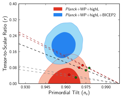
Figure 4: Marginalized joint $68\%$ and $95\%$ CL regions for ($n_{s}$, $r$), using observational data sets with and without a running spectral index, compared to the theoretical prediction of the model (73) with $n=1$. The black dashed line is for the case where model parameter $\alpha=0$ while gray and brown are for the case where $\alpha=-0.003$ and $\alpha=0.001$, respectively. The pairs of red and green dots represent the number of $e$-folds, $N=50$ and $N=60$, respectively.

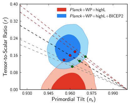
Figure 5: Marginalized joint $68\%$ and $95\%$ CL regions for ($n_{s}$, $r$), using observational data sets with and without a running spectral index, compared to the theoretical prediction of the model (73) with $n=2$. The black dashed line is for the case where model parameter $\alpha=0$ while gray and brown are for the case where $\alpha=-2\times 10^{-6}$ and $\alpha=1.5\times 10^{-6}$, respectively. The pairs of red and green dots represent the number of $e$-folds, $N=50$ and $N=60$, respectively.

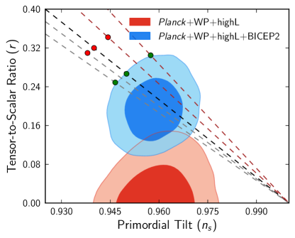
Figure 6: Marginalized joint $68\%$ and $95\%$ CL regions for ($n_{s}$, $r$), using observational data sets with and without a running spectral index, compared to the theoretical prediction of the model (73) with $n=4$. The black dashed line is for the case where model parameter $\alpha=0$ while gray and brown are for the case where $\alpha=-0.7\times 10^{-12}$ and $\alpha=1.5\times 10^{-12}$, respectively. The pairs of red and green dots represent the number of $e$-folds, $N=50$ and $N=60$, respectively.

In Table 1, we list the range of the model parameter $\alpha$ in which the predicted value of $n_{s}$ and $r$ is consistent with Planck + BICEP2.

Table 1: Observationally favored range of model parameters $\alpha$ for different values of $n$ and $N$ from the observational data set.

Model	Parameter range	Parameter range
$n$	for N=50	for N=60
n=1	$-6.6\times 10^{-3}\leq\alpha\leq 2\times 10^{-3}$	$-5.5\times 10^{-3}\leq\alpha\leq 4\times 10^{-4}$
n=2	$-5.2\times 10^{-6}\leq\alpha\leq 6\times 10^{-6}$	$-3.2\times 10^{-6}\leq\alpha\leq 1.5\times 10^{-6}$
n=4	${\small\mbox{lies outside of }2\sigma\mbox{ boundary}}$	$-0.7\times 10^{-12}\leq\alpha\leq 1.5\times 10^{-12}$

We plot the $dn_{s}/d\ln k$ with $n_{s}$ in Figs. 7–9. The theoretical prediction from (93) is $|\frac{dn_{s}}{d\ln k}|\sim 10^{-4}$, but Planck combined with the BICEP2 data provides $|\frac{dn_{s}}{d\ln k}|\sim 10^{-2}$, which is larger than the theoretical predictions. Therefore, the predictions of our model lie outside of $95\%$ regions. Meanwhile, the model predictions are consistent with Planck alone with or without the running spectral index at $95\%$ CL. We may understand this as follows: As we explained in Sec. I, we consider the running spectral index of the scalar modes as a simple resolution to reconcile BICEP2 with Planck, which was considered in Ref. Ade:2014xna . Either our theoretical model is not consistent with the observations under the assumption that the BICEP2 data is correct or considerations of the running spectral index may not be the right resolution to reconcile both data.

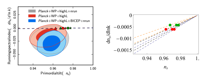
Figure 7: $n_{s}$ vs $dn_{s}/d\ln k$ plot, with observational data sets (left) and without observational data sets (right), compared to the theoretical prediction of the model (73) with $n=1$. The black dashed line is for the case where model parameter $\alpha=0$ while orange and blue are for the case where $\alpha=-0.003$ and $\alpha=0.001$, respectively. The pairs of red and green markers represent the number of $e$-folds, $N=50$ and $N=60$, respectively.

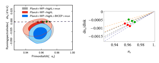
Figure 8: $n_{s}$ vs $dn_{s}/d\ln k$ plot, with observational data sets (left) and without observational data sets (right), compared to the theoretical prediction of the model (73) with $n=2$. The black dashed line is for the case where model parameter $\alpha=0$ while orange and blue are for the case where $\alpha=-2\times 10^{-6}$ and $\alpha=1.5\times 10^{-6}$, respectively. The pairs of red and green markers represent the number of $e$-folds, $N=50$ and $N=60$, respectively.

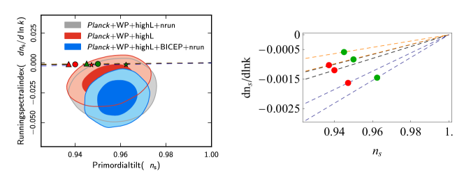
Figure 9: $n_{s}$ vs $dn_{s}/d\ln k$ plot, with observational data sets (left) and without observational data sets (right), compared to the theoretical prediction of the model (73) with $n=4$. The black dashed line is for the case where model parameter $\alpha=0$ while orange and blue are for the case where $\alpha=-10^{-12}$ and $\alpha=2.5\times 10^{-12}$, respectively. The pairs of red and green markers represent the number of $e$-folds, $N=50$ and $N=60$, respectively.

Therefore, we need to find another way to resolve the inconsistency with BICEP2 data since our predictions are not consistent with the $dn_{s}/d\ln k$-$n_{s}$ data. We will leave it for a future work because these considerations are beyond the scope of this work.

V Conclusions and discussions

We have investigated the slow-roll inflation with the Gauss-Bonnet term that is coupled to the inflaton field nonminimally. We have considered the potential and coupling function as $V(\phi)=V_{0}e^{\lambda\phi},\,\,\xi(\phi)=\xi_{0}e^{\lambda\phi}$ (Sec. IV.1) and $V(\phi)=V_{0}\phi^{n},\,\,\xi(\phi)=\xi_{0}\phi^{n}$ (Sec. IV.2), respectively, to relax the condition $V(\phi)\xi(\phi)={\rm const.}$, which was widely studied in Refs. Guo:2010jr –Jiang:2013gza . $N\simeq 60$ condition requires that $\alpha\simeq 10^{-6}$ for $V\sim\phi^{2}$ and $\alpha\simeq 10^{-12}$ for $V\sim\phi^{4}$ (see Fig. 2) where $\alpha=\frac{4}{3}\kappa^{4}V_{0}\xi_{0}$.

The power spectra of the scalar and tensor perturbations were analytically derived in (51) and (52), respectively, with the slow-roll approximation. Observational quantities such as the spectral indices of the scalar and tensor modes, the tensor-to-scalar ratio, and the running spectral indices of the scalar and tensor modes are calculated using these power spectra to compare with the recent CMB observation data, Planck, and BICEP2.

Regarding the tensor-to-scalar ratio, $r$, the Planck+WMAP data provide the upper bound on $r<0.12$, but the BICEP2 observation that detected the B-mode polarization gives $r=0.2$. It seems at first sight that there is some mismatch between two observations. In Ref.Ade:2014xna , they suggested considering the running spectral index to reconcile BICEP2 with Planck. Although there has been wide study to explain this discrepancy, we consider in this work the running spectral index of the scalar perturbation by accepting the simple resolution of the discrepancy between two data.

First, we have applied our general formalism to the large-field inflationary model with the exponential potential with exponential Gauss-Bonnet coupling (62). In the presence of the Gauss-Bonnet term, we could find the valid model parameter ranges for inflation to happen, unfortunately, these parameter ranges are not favored by the data. Second, we have studied the large-field inflationary model with the monomial potential with monomial Gauss-Bonnet coupling (73). In this scenario, $r$ is enhanced for $\alpha>0$ while it is suppressed for $\alpha<0$. This result is completely opposite compared to Refs. Guo:2010jr –Jiang:2013gza , in which $r$ is enhanced for $\alpha<0$ and reduced for $\alpha>0$ for the model with potential, $V=V_{0}\phi^{n}$, and Gauss-Bonnet coupling, $\xi=\xi_{0}\phi^{-n}$.

As shown in Figs. 4–6, the model parameter $\alpha$ can shift the predicted $r$ value vertically for the fixed number of $e$-folds in $n_{s}$-$r$ plane. For $n=1$, the theoretical predictions can be made to better fit to Planck data. However, this type of model is not favored by the recent Planck+BICEP2 data. For $n=2$, the model with the quadratic potential can be made a better fit to the recent Planck+BICEP2 data within a certain parameter range given in Table 1. In the model with $n=4$ for $\alpha=0$, it is well known that this scenario of inflation is excluded by the Planck data. However, the predictions with $\alpha\neq 0$ for $n=4$ lie inside of the $2\sigma$ contour for $N\gtrsim 60$.

However, among the model predictions in this work, $dn_{s}/d\ln k$ turns out to be inconsistent with BICEP2 combining with the Planck data that lie outside of $2\sigma$ contour of the BICEP2+Planck data. It would be interesting to search for the alternatives to reconcile Planck data with BICEP2 besides consideration of the running spectral index. We will leave it as a future work whether there are any solutions for our model to satisfy both the BICEP2 and Planck data without considering $dn_{s}/d\ln k$.

- (1) P. A. R. Ade et al. (Planck Collaboration), Astron. Astrophys. 566, A54 (2014).
- (2) S. Chatrchyan et al. (CMS Collaboration), Phys. Lett. B 716, 30 (2012); G. Aad et al. (ATLAS Collaboration), Phys. Lett. B 716, 1 (2012)
- (3) P. A. R. Ade et al. (BICEP2 Collaboration), Phys. Rev. Lett. 112, 241101 (2014)
- (4) A. Ijjas, P. J. Steinhardt, and A. Loeb, Phys. Lett. B 723, 261 (2013); A. H. Guth, D. I. Kaiser, and Y. Nomura, Phys. Lett. B 733, 112 (2014); A. Ijjas, P. J. Steinhardt, and A. Loeb, Phys. Lett. 07B, 12 (2014)
- (5) P. A. R. Ade et al. (Planck Collaboration), arXiv:1303.5082.
- (6) M. -J. Motonson and U. Seljak, arXiv:1405.5857v1.
- (7) R. -Flauger, J. C. Hill, and D. N. Spergel, arXiv:1405.5857v1.
- (8) C. G. Callan, Jr., E. J. Martinec, M. J. Perry, and D. Friedan, Nucl. Phys. B262, 593 (1985); D. J. Gross and J. H. Sloan, Nucl. Phys. B291, 41 (1987); B. Zwiebach, Phys. Lett. B156, 315 (1985).
- (9) I. Antoniadis, E. Gava, and K. S. Narain, Nucl. Phys. B383, 93 (1992); I. Antoniadis, J. Rizos, and K. Tamvakis, Nucl. Phys. B415, 497 (1994); S. Kawai, M. -a. Sakagami, and J. Soda, Phys. Lett. B 437, 284 (1998)
- (10) S. W. Hawking and R. Penrose, Proc. R. Soc. Lond. A 314, 529 (1970).
- (11) J. -C. Hwang and H. Noh, Phys. Rev. D 61, 043511 (2000).
- (12) S. Kawai and J. Soda, Phys. Lett. B 460, 41 (1999).
- (13) M. Satoh, S. Kanno, and J. Soda, Phys. Rev. D 77, 023526 (2008).
- (14) M. Satoh and J. Soda, J. Cosmol. Astropart. Phys. 09, (2008) 019.
- (15) M. Satoh, J. Cosmol. Astropart. Phys. 11, (2010) 024.
- (16) Z. -K. Guo and D. J. Schwarz, Phys. Rev. D 81, 123520 (2010).
- (17) P. -X. Jiang, J. -W. Hu and Z. -K. Guo, Phys. Rev. D 88, 123508 (2013).
- (18) J. -C. Hwang and H. Noh, Phys. Rev. D 71, 063536 (2005).