An analytical approach to the external force-free motion of pendulums on surfaces of constant curvature

Abstract

The dynamics of force free motion of pendulums on surfaces of constant Gaussian curvature is addressed when the pivot moves along a geodesic obtaining the Lagragian of the system. As a application it is possible the study of elastic and quantum pendulums.

AMS classification scheme numbers: 70H03, 53A35, 53B20.

Keywords: Dynamical systems, Lagrangian and Hamiltonian mechanics, Semi-Riemannian geometry, constant curvature, pendulum.

1 Introduction

The classical theory of force-free motions of rigid particle systems has a long history in connection with investigation in Mathematics and Mechanics. From the Differential Calculus, in the case of translational particle motions in Euclidean space (Newton axioms of Mechanics), to the Riemann Geometry. Hence, the definition of geodesics has immediately concerned with force-free particle motions on surfaces. The introduction of Riemannian manifolds and the geometry of their geodesics were motivated by the mechanics of constrained particle systems. In the last few years, the study of force-free motion systems on Riemannian manifolds of constant sectional curvature has attracted the interest of several authors [1], [2], [3], [6], [7] and [8].

In particular, in [2] the authors define the notion of a pendulum on a surface of constant Gaussian curvature $K$ and they study the motion of a mass at a fixed distance from a pivot. So, a pendulum problem on a surface of constant curvature is defined as a pivot point and a mass connected to that point by a rigid massless rod of fixed length $\rho$. It is assumed that the pivot is constrained to move along some fixed curve with prescribed motion. The rod provides the only force on the mass in order to keep the mass at the fixed distance from the pivot. No torque is applied to the rod, (fig. 1). In [2] it is studied the pendulum problem when the pivot moves along a geodesic path, and the space is a surface of constant (not zero) curvature. It is considered the surface immersed in $\mathds{R}^{3}$ or $\mathds{L}^{3}$ and it is obtained the differential motion equation by Newtonian procedure doing a laborious calculation. Moreover, the cases $K>0$ and $K<0$ are necessary to come from different forms.

In this work, we deal with the pendulum problem from an analytic point of view. This procedure allows approach simultaneously the cases of positive and negative curvature and also of zero curvature (as a limit case), with very simple computations. The key of our study is a lagragian approach, which has a 1-dimensional configuration space. As adirect consequence the internal curvature force is conservative and its potential function is easily calculated. Moreover, this method can be used to another related problems, as the elastic pendulum, or the quantum pendulum.

Mainly, this work concerns the case in which the pivot moves along a geodesic. Let $\zeta$ be the angle between the rod and the motion direction of the pivot. We will assume the following convention:

If the constant curvature of the space is $K>0$,

$$\cos_{K}(z)=\cos(z\sqrt{K}),\quad\sin_{K}(z)=\sin(z\sqrt{K}),\quad\tan_{K}(z)=\tan(z\sqrt{K})\,.$$

If the constant curvature of the space is $K<0$,

$$\cos_{K}(z)=\cosh(z\sqrt{-K}),\quad\sin_{K}(z)=\sinh(z\sqrt{-K}),\quad\tan_{K}(z)=\tanh(z\sqrt{-K})$$

The main result is the following:

Suppose that the pivot of pendulum moves with constant speed $v$ along a geodesic on a surface with constant curvature $K$. Let $\zeta(t)$ the angle at the time $t$ between the rigid rod and the direction of pivot motion. Then the Lagrangian of the system is

$${\cal L}(\zeta,\dot{\zeta})=\frac{1}{2}m\dot{\zeta}^{2}\sin_{K}^{2}(\rho)\frac{1}{\mid K\mid}-\frac{1}{2}mv^{2}{\rm sgn}(K)\sin_{K}^{2}(\rho)\sin^{2}(\zeta).$$

Therefore, the motion equation is

$$\frac{d^{2}\zeta}{dt^{2}}=-v^{2}K\sin_{K}(\zeta)\cos_{K}(\zeta).$$ (1)

Using the previous result and geometric arguments, we obtain the motion equation of the system when the pivot accelerates along a geodesic (see Section 4). Further developements are discussed in Section 5.

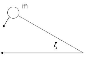
Figure 1: Pendulum motion

2 Preliminaries

It is well known that a complete, simply-connected Riemannian $n$-manifold with constant sectional curvature is isometric to one of model spaces $\mathds{R}^{n}$, $\mathds{S}^{n}(R)$ or $\mathds{H}^{n}(R)$ (see [5]).

Let $(\mathds{S}^{2}(R),\langle\,,\,\rangle_{1})$ be the 2-dimensional sphere of radius $R$, endowed with the metric induced from $(\mathds{R}^{3},\langle\,,\,\rangle)$, where

$$\langle\,,\,\rangle=dx^{2}+dy^{2}+dz^{2}.$$

Consider the coordinate system $\{U_{1},\Phi=(\varphi,\theta)\}$ in $S^{2}(R)$ with $U_{1}=\Phi^{-1}((0,\pi)\times(0,2\pi))$ and $\Phi^{-1}(\varphi,\theta)=(x,y,z)$, being

$$\left.\begin{array}[]{l}x=R\sin{\varphi}\cos{\theta}\\ y=R\sin\varphi\sin\theta\\ z=R\cos\varphi\end{array}\right\}$$

In this coordinate system the metric is given by

$$\langle\,,\,\rangle_{1}=R^{2}\,d\varphi\otimes d\varphi+R^{2}\sin^{2}\varphi\,d\theta\otimes d\theta,$$

and the non-zero Christoffel symbols are $\Gamma_{\varphi\theta}^{\theta}=\cot\varphi$ and $\Gamma_{\theta\theta}^{\varphi}=-\sin\varphi\cos\varphi$.

Let’s consider also the hyperbolic plane $(\mathds{H}^{2}(R),\langle\,,\,\rangle_{2})$, where

$$\mathds{H}^{2}(R)=\{(x,y,z)\in\mathds{R}^{3}/x^{2}+y^{2}-z^{2}=-R^{2}\}$$

and $\langle\,,\,\rangle_{2}$ is the induced metric from the Lorentz-Minkowski spacetime $\mathds{L}^{3}$.

Let $\{U_{2},\Psi=(\alpha,\beta)\}$ be the coordinate system in $\mathds{H}^{2}(R)$ with $U_{2}=\Psi^{-1}((-\infty,\infty)\times(-\infty,\infty))$ and $\Psi^{-1}(\alpha,\beta)=(x,y,z)$, where

$$\left.\begin{array}[]{l}x=R\cosh{\alpha}\sinh{\beta}\\ y=R\sinh\alpha\\ z=R\cosh\alpha\cosh\beta\end{array}\right\}$$

The metric is given by

$$\langle\,,\,\rangle_{2}=R^{2}d\alpha\otimes d\alpha+R^{2}\sinh^{2}\alpha\,d\beta\otimes d\beta$$

and the non-zero Christoffel symbols are $\Gamma_{\alpha\beta}^{\beta}=\coth\alpha$ and $\Gamma_{\beta\beta}^{\alpha}=-\sinh\alpha\cosh\beta$.

3 Rigid pendulum

Firstly, we deal with the rigid pendulum problem in the case that the pivot moves along a geodesic of its space, with constant speed. We will do analogously the study for $K>0$ and $K<0$.

3.1 Spherical case, kinetic energy

Note that in the case $K>0$ we must require that $\rho<\pi R$ to guarantee that the mass and the rod are on the same side of the geodesic line.

Suppose that the pivot moves along the geodesic $\varphi=\frac{\pi}{2}$ with constant speed. Let’s take a reference associated to the pivot. Denote by $\zeta$ the angle between the rigid rod and the direction of pivot motion.

The Lagrangian of the system has two components, on the one hand, the kinetic energy of the mass ${\bf T}$, and on the other hand, the potential energy ${\bf V}$, which is due to the curvature of space, i.e., ${\bf V}=0$ if the space is flat.

Consider the isosceles geodesic triangle formed in an infinitesimal temporal interval, by the rod and the arc $dl$ traced by the mass (fig. 2).

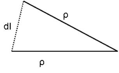
Figure 2: Infinitesimal triangle

The Sine Theorem for Spherical Geometry allows us to write

$$dl=R\,\sin(\rho/R)\,d\zeta=\frac{1}{\sqrt{\mid K\mid}}\sin(\rho\sqrt{\mid K\mid})\,d\zeta,$$

thus

$$\tilde{v}=\frac{dl}{dt}=\dot{\zeta}\sin(\rho\sqrt{\mid K\mid})\frac{1}{\sqrt{\mid K\mid}}.$$

Therefore, if the particle has mass $m$, the kinetic energy is given by

$${\bf T}=\frac{1}{2}m\dot{\zeta}^{2}\sin^{2}(\rho\sqrt{\mid K\mid})\frac{1}{{\mid K\mid}}.$$

3.2 Spherical case, potential energy

Consider the coordinate system $\{U_{1},\Phi=(\varphi,\theta)\}$ with the metric $\langle\,,\,\rangle_{1}=R^{2}\,d\varphi\otimes d\varphi+R^{2}\sin^{2}\varphi\,d\theta\otimes d\theta,$ and suppose that the pivot moves along the geodesic $\varphi=\frac{\pi}{2}$ with constant speed $v$. Obtain us the mass acceleration due to the curvature, so suppose that the mass moves along the curve

$$\left.\begin{array}[]{l}\varphi=\varphi_{0}\\ \theta=\frac{v}{R}t\end{array}\right\}$$

Its acceleration is given by

$$a=\frac{v^{2}}{R^{2}}\Gamma_{\theta\theta}^{\varphi}\frac{\partial}{\partial\varphi}=-\frac{v^{2}}{R^{2}}\sin(\varphi)\cos(\varphi)\frac{\partial}{\partial\varphi}.$$

As consequence, the external force that we must be to apply on the rod will be ${\bf F}_{e}=ma$ and the curvature potential energy ${\bf V}$ satisfies ${\bf F}=-{\rm grad}\,({\bf V})$, where ${\bf F}=-{\bf F}_{e}$. Hence,

$${\bf V}=\int_{\pi/2}^{\varphi}R^{2}(-m\sin(\varphi)\cos(\varphi))\frac{v^{2}}{R^{2}}\,d\varphi=\frac{m}{2}v^{2}\cos^{2}\varphi$$

where we have taken $\pi/2$ as origin energy. Again, using the Sine Theorem (fig. 3) we obtain

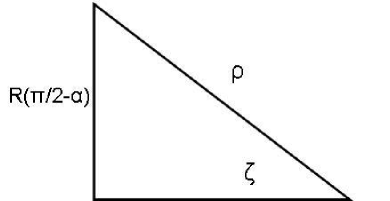
Figure 3: Geodesic triangle

$$\cos(\varphi)=\sin(\zeta)\sin(\rho/R).$$

Thus

$${\bf V}(\zeta)=-\frac{m}{2}v^{2}\sin^{2}(\rho/R)\sin^{2}(\zeta).$$

Now, we can enunciate the following Theorem,

Theorem 3.1

Suppose that the pivot of pendulum moves with constant speed $v$ along a geodesic on a surface with constant curvature $K>0$. Let $\zeta(t)$ the angle at the time $t$ between the rigid rod and the direction of pivot motion. Then the Lagrangian of the system is

$${\cal L}(\zeta,\dot{\zeta})=\frac{1}{2}m\dot{\zeta}^{2}\sin^{2}(\rho/R)\frac{1}{K}-\frac{1}{2}mv^{2}\sin^{2}(\rho/R)\sin^{2}(\zeta)$$ (2)

Therefore, the motion differential equation is given by

$$\frac{d^{2}\zeta}{dt^{2}}=-v^{2}K\sin(\zeta)\cos(\zeta)$$ (3)

If we do $K\rightarrow 0$,

$$\sin(\rho)\simeq\rho\sqrt{\mid K\mid}$$

and

$$\lim_{K\rightarrow 0}{\cal L}=\frac{1}{2}m\dot{\zeta}^{2}\rho^{2},$$

obtaining the Lagrangian function of the pendulum moving in the Euclidean plane, when the pivot moves along a straigh line with constant speed.

3.3 Hyperbolic case, kinetic energy

Consider us now, the pivot moving along the geodesic $\alpha=0$, with constant speed $v$. Analogously to the spherical case, we take a reference joint with the pivot and we denote $\zeta$ the angle between the rigid rod and the direction of pivot motion.

If we consider the isosceles hyperbolic differential triangle (fig. 2), and making use of the corresponding theorems of the Hyperbolic Geometry, we can to conclude that the kinetic energy of the system is given by

$${\bf T}=\frac{m}{2}\dot{\zeta}^{2}\sinh(\rho/R)\,\frac{1}{\mid K\mid}.$$

3.4 Hyperbolic case, potential energy

Reasoning as the in spherical case, we consider that the pivot moves along the geodesic $\alpha=0$. If the mass moves along the curve

$$\left.\begin{array}[]{l}\alpha=\alpha_{0}\\ \beta=\frac{v}{R}t\end{array}\right\},$$

we can to calculate the curvature potential function,

$${\bf V}=\int_{0}^{\alpha}R^{2}(-m\sinh(\alpha)\cosh(\alpha))\frac{v^{2}}{RÂ\texttwosuperior}=-\frac{m}{2}v^{2}\sinh(\alpha)\,,$$

where we have taken $0$ as origin energy. Again, using the Sine Theorem in the hyperbolic case, we obtain

$$\sinh(\alpha)=\sin(\zeta)\sinh(\rho/R).$$

Thus,

$${\bf V}=-\frac{m}{2}v^{2}\sinh^{2}(\rho/R)\sin^{2}(\zeta).$$

Theorem 3.2

Suppose that the pivot of the pendulum moves with constant speed $v$ along a geodesic on a surface with constant curvature $K<0$. Let $\zeta(t)$ the angle at the time $t$ between the rigid rod and the direction of pivot motion. Then the Lagrangian of the system is given by

$${\cal L}(\zeta,\dot{\zeta})=\frac{1}{2}m\dot{\zeta}^{2}\sinh^{2}(\rho/R)\frac{1}{\mid K\mid}+\frac{1}{2}mv^{2}\sinh^{2}(\rho/R)\sin^{2}(\zeta).$$ (4)

Therefore, the motion differential equation is

$$\frac{d^{2}\zeta}{dt^{2}}=v^{2}\mid K\mid\sinh(\zeta)\cosh(\zeta).$$ (5)

With our convention, we can to enunciate (compare with [2], Theorem A):

Theorem 3.3

Suppose that the pivot of pendulum moves with constant speed $v$ along a geodesic on a surface with constant curvature $K$. Let $\zeta(t)$ the angle at the time $t$ between the rigid rod and the direction of pivot motion. Then the Lagrangian of the system is given by

$${\cal L}(\zeta,\dot{\zeta})=\frac{1}{2}m\dot{\zeta}^{2}\sin_{K}^{2}(\rho)\frac{1}{\mid K\mid}-\frac{1}{2}mv^{2}{\rm sgn}(K)\sin_{K}^{2}(\rho)\sin^{2}(\zeta).$$

Therefore, the motion differential equation is

$$\frac{d^{2}\zeta}{dt^{2}}=-v^{2}K\sin_{K}(\zeta)\cos_{K}(\zeta).$$

Remark 3.4

Suppose $K>0$ and consider the motion equation (3). Making the change $u=2\zeta$, we obtain the differential equation

$$\frac{d^{2}u}{dt^{2}}=-v^{2}K\sin(u),$$ (6)

which is the equation of planar pendulum of length $1$ in Euclidean space subject to a constant gravitational field of magnitude $g=v^{2}K$. Its stable and unstable equilibria at $u=0$ and $u=\pi$, correspond to the stable $\zeta=0$ and unstable $\zeta=\pi/2$ equilibria of the pendulum on the spherical surface.

On the other hand, if $K<0$, making $u=\pi-2\zeta$ in the motion equation (5), we obtain, in similar form, that $\zeta=\pi/2$ is stable equilibria and $\zeta=0$ is unstable equilibria.

Moreover, it is well known that the equation (6) can be exactly solved in term of a elliptic integral of first kind (see [9], for instance), which cannot be evaluated in a closed form.

A first approximation to this problem in arbitrary constant curvature is given for small oscillations around the stable equilibria points of this physical system. That is, for small $u$, $\sin_{K}u\simeq u$, and the equation of motion is approximated by

$$\frac{d^{2}u}{dt^{2}}=-v^{2}\mid K\mid u.$$

Observe that the previous equation represents a simple harmonic oscillator of frequence $\omega=v\sqrt{\mid K\mid}$.

3.5 A first integral

Since the Hamiltonian function ${\cal H}$ is time independent, it is an integral on phase space and it represents the system energy. Using the standard notation $(q_{\zeta},p_{\zeta})$ in the phase space, we can write

$$p_{\zeta}=\frac{\partial{\cal L}}{\partial\dot{\zeta}}=m\dot{\zeta}\sin^{2}_{K}(\rho)\frac{1}{\mid K\mid}.$$

The Legendre transformations allow us to give

$${\cal H}(\zeta,\dot{\zeta})=\frac{1}{2}m\dot{\zeta}^{2}\sin_{K}^{2}(\rho)\frac{1}{\mid K\mid}+\frac{1}{2}mv^{2}{\rm sgn}(K)\sin_{K}^{2}(\rho)\sin^{2}(\zeta).$$ (7)

Moreover, it is easy to see that ${\cal H}$ is constant if and only if

$$2\Big{(}\frac{d\zeta}{dt}\Big{)}^{2}-Kv^{2}\cos(2\zeta)$$

is constant (compare with [2, Prop. 1]).

4 Accelerated pivot

Suppose now that the pivot moves along a geodesic path with lineal acceleration $a(t)$. We come to compute the acceleration induced by the accelerated pivot at the mass making use of a geometric argument. We follow the following steps:

a) Translate to the mass the pivot acceleration $a(t)$ .

b) Transform this acceleration in angular acceleration between the rod and the geodesic path traced by the pivot.

c) Project on the orthogonal direction to the rod.

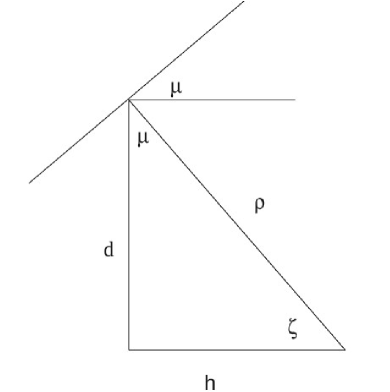
Figure 4: Triangle

Indeed, consider the geodesic triangle of the figure 4. The translated acceleration to the mass is given by

$$a(t)\cos_{K}(d),$$

and the angular acceleration by

$$\frac{a(t)\cos_{K}(d)}{R\sin_{K}(\rho)}.$$

Finally, in order to project, it is enough to multiply by $\cos(\mu)$

$$\frac{a(t)\cos_{K}(d)\cos(\mu)}{R\sin_{K}(\rho)}.$$

On another hand, taking into account the previous triangle, from the Pythagoras and Cosine Theorem in non-Euclidean geometries, we have

$$\cos_{K}(\mu)=\sin_{K}(\zeta)\cos_{K}(h)\ \ {\rm and}\ \ \cos_{K}(\rho)=\cos_{K}(d)\cos_{K}(h),$$

thus $\cos_{K}(d)\cos_{K}(\mu)=\cos_{K}(\rho)\sin_{K}(\zeta)$. As a consequence, the searched acceleration is

$$\sqrt{\mid K\mid}a(t)\cot_{K}(\rho)\sin_{K}(\zeta(t)).$$

So, we prove in a different approach the result ([2, Theorem D])

Theorem 4.1

Assume that the pivot moves with speed $v(t)$ along a geodesic on a surface with constant curvature $K$. Let $\zeta(t)$ the angle that the rigid rod makes with the direction of the motion of the pivot. Then the pendulum satisfies the differential equation

$$\frac{d^{2}\zeta}{dt^{2}}=-v(t)^{2}K\sin(\zeta(t))\cos(\zeta(t))+\sqrt{\mid K\mid}\,a(t)\,{\rm cotan}_{K}(\rho)\,\sin(\zeta(t)),$$

where $a(t)=\frac{dv}{dt}.$

5 Some further physical applications

As a first application, consider us the case of a pendulum whose pivot moves along a geodesic on a surface of constant curvature with constant speed $v$ and whose rod is elastic. Let $k$ be the elastic constant of the rod, let $\rho$ be the length of the rod and let $l(t)$ be the elongation of the rod at the time $t$. Our analytical approach allows us to initiate the study of dynamical system in similar form as the rigid case. So, it is not difficult to see that its Lagrangian function is given by

$${\cal L}(\zeta,l,\dot{\zeta},\dot{l})=\frac{1}{2}m\dot{\zeta}\sin_{K}^{2}(\rho+l)\frac{1}{|K|}-\frac{1}{2}mv^{2}{\rm sgn}(K)\sin^{2}_{K}(\rho+l)\sin_{K}^{2}(\zeta)+\frac{1}{2}m\dot{l}^{2}-\frac{1}{2}kl^{2}$$

Secondly, we will make an approximation to the quantum system. Denote $\overline{m}:=m\sin_{K}^{2}(\rho)/\mid K\mid$. Then, (7) can be written, for $K>0$, in terms of $\zeta$ and $p_{\zeta}$ as

$${\cal H}(\zeta,p_{\zeta})=\frac{p_{\zeta}^{2}}{2\overline{m}}+\frac{1}{2}\overline{m}v^{2}K\sin^{2}(\zeta).$$

Observe that the same expression, up an additive term, is obtained for $K<0$. Therefore, a suitable time independient Schrodinger equation for this system can be described as

$$-\frac{\hbar^{2}}{2\overline{m}}\frac{d^{2}\psi}{d\zeta^{2}}+\frac{1}{2}\overline{m}v^{2}K\sin^{2}(\zeta)\psi=E\psi,$$

where $\psi(\zeta)$ is a complex function representing the wave function of the mass particle in this physical system. Observe that it is expected that the energy should take quantized values. In fact, if it is assumed that $\psi$ is confined in a region where $\zeta$ is close to $0$, the previous equation, in this first approximation, corresponds to the quantum harmonic oscillator, whose energy is found to be

$$E_{n}=\hbar v\sqrt{|K|}\left(n+\frac{1}{2}\right),\ \ {\rm for\ \ all}\ \ n\in\mathbb{N}.$$

Observe that, within this simplification, in the quantum of energy, $\hbar v\sqrt{|K|}$, appears the speed of the rod and the curvature of the ambient space.

References

- [1] Cariñera J. F., Rañada M. F. and Santander M. The harmonic oscillator on Riemannian and Lorentzian configuration spaces of constant curvature J. Math. Phys. 49 (2008), 032703, 27 pp.
- [2] Coulton P., Foote R. and Galpering The dynamics of pendulums on surfaces of constant curvature Math. Phys. Anal. Geom. 12 (2009 ), 97–107.
- [3] Coulton P., Foote R. and Galpering Forces along equidistant particle paths Math. Phys. Anal. Geom. 7 (2004), 187–192.
- [4] Kozlov V. V. and Harin A. O. Kepler’s problem in constant curvature spaces Celestial Mechanics and Dynamical Astronomy 54 (1992), 393–399
- [5] Lee J. M: Riemannian Manifolds. An introduction to Curvature, (1997) Springer.
- [6] Lazarte M.M., Salvai M. and Will A., Force free projective motions of the sphere, J. Geom. Phys. 57 (2007), 2431–2436.
- [7] Nagy P.T., Dynamical invariants of rigid motions on the hyperbolic plane, Geom. Dedicata 37 (1991), 125–139.
- [8] Salvai M., Force free conformal motions of the sphere, Differential Geometry and its Applications 16 (2002), 285–292.
- [9] Sankara K. Classical Mechanics (2005), Prentice Hall of India.