A mass-dependent density profile for dark matter haloes including the influence of galaxy formation

Abstract

We introduce a mass dependent density profile to describe the distribution of dark matter within galaxies, which takes into account the stellar-to-halo mass dependence of the response of dark matter to baryonic processes. The study is based on the analysis of hydrodynamically simulated galaxies from dwarf to Milky Way mass, drawn from the MaGICC project, which have been shown to match a wide range of disk scaling relationships. We find that the best fit parameters of a generic double power-law density profile vary in a systematic manner that depends on the stellar-to-halo mass ratio of each galaxy. Thus, the quantity ${{M_{\star}}}/{{M_{\rm halo}}}$ constrains the inner ($\gamma$) and outer ($\beta$) slopes of dark matter density, and the sharpness of transition between the slopes ($\alpha$), reducing the number of free parameters of the model to two. Due to the tight relation between stellar mass and halo mass, either of these quantities is sufficient to describe the dark matter halo profile including the effects of baryons. The concentration of the haloes in the hydrodynamical simulations is consistent with N-body expectations up to Milky Way mass galaxies, at which mass the haloes become twice as concentrated as compared with pure dark matter runs.

This mass dependent density profile can be directly applied to rotation curve data of observed galaxies and to semi analytic galaxy formation models as a significant improvement over the commonly used NFW profile.

1 Introduction

Over several orders of magnitude in radius, dark matter (DM) halo density profiles arising from N-body simulations are well described by the so-called ’NFW’ model (Navarro et al., 1996; Springel et al., 2008; Navarro et al., 2010), albeit with well known systematic deviations (e.g., Navarro et al., 2004; Springel et al., 2008; Gao et al., 2008; Navarro et al., 2010; Dutton & Macciò, 2014). The NFW function consists of two power laws, the inner region where the density is behaving as $\rho\propto r^{-1}$ and the outer part as $\rho\propto r^{-3}$.

The central $\rho\propto r^{-1}$ “cusps” of such model disagree with observations of real galaxies where mass modeling based on rotation curves finds much shallower inner density slopes, known as “cored” profiles (e.g., Moore, 1994; Salucci & Burkert, 2000; de Blok et al., 2001; Simon et al., 2005; de Blok et al., 2008; Kuzio de Naray et al., 2008; Kuzio de Naray et al., 2009; Oh et al., 2011). Cored galaxies are also found within the fainter, dark matter dominated dwarfs spheroidal galaxies surrounding the Milky Way (Walker & Peñarrubia, 2011). This cusp/core discrepancy is usually seen as one of the major problems of the $\Lambda$CDM paradigm at small scales.

The NFW profile is, however, derived from pure DM simulations in which particles only interact through gravity. These simulations neglect hydrodynamical processes that may be relevant in determining the inner halo profile. Many studies have shown how baryons can affect the dark matter. Gas cooling to the center of a galaxy causes adiabatic contraction (e.g. Blumenthal et al., 1986; Gnedin et al., 2004), whose effect strengthens cusps and exacerbates the mismatch between theoretical profiles and observations. Rather, expanded haloes are required to reconcile observed galaxy scaling relations of both early and late-type galaxies (Dutton et al., 2007, 2013).

Baryons can expand haloes through two main mechanisms (see Pontzen & Governato (2014) for a recent review): outflows driven by stellar or AGN feedback (Navarro et al., 1996; Mo & Mao, 2004; Read & Gilmore, 2005; Mashchenko et al., 2006; Duffy et al., 2010; Pontzen & Governato, 2012; Martizzi et al., 2013) and dynamical friction (El-Zant et al., 2001; Tonini et al., 2006; Romano-Díaz et al., 2008; Del Popolo, 2009, 2010; Goerdt et al., 2010; Cole et al., 2011).

While dynamical friction is effective at expanding high mass haloes hosting galaxy clusters, stellar feedback is most effective at expanding low mass haloes (Governato et al., 2010). Gas cools into the galaxy centre where it forms stars that drive repeated energetic outflows. Such outflows move enough gas mass to create a core in an originally cuspy dark halo, due to the DM response to the adjusted gravitational potential. Peñarrubia et al. (2012) calculated the energy required to flatten a density profile as a function of halo mass. The cusp/core change can be made permanent if the outflows are sufficiently rapid (Pontzen & Governato, 2012).

Simulations from dwarf galaxies (Governato et al., 2010; Zolotov et al., 2012; Teyssier et al., 2013) to Milky Way mass (Macciò et al., 2012) have produced dark matter halo expansion depending on the implementation of stellar feedback. Governato et al. (2012) showed that only simulated galaxies with stellar masses higher than $\sim 10^{7}M_{\odot}$ expand their haloes. They also showed that the inner DM profile slope, $\gamma$ in $\rho\propto r^{-\gamma}$, flattens with increasing stellar mass, resulting from the increase of available energy from supernovae. An increase in stellar mass may, however, also deepen the potential well in the central region of the halo: indeed, Di Cintio et al. (2014) showed that above a certain halo mass such a deepened potential well opposes the flattening process.

Di Cintio et al. (2014) propose that $\gamma$ depends on the stellar-to-halo mass ratio of galaxies. At ${{M_{\star}}}/{{M_{\rm halo}}}\mathrel{\hbox{\hbox to0.0pt{\hbox{\lower 4.0pt\hbox{$\sim$}}\hss}\hbox{$<$}}}10^{-4}$ there is not enough supernova energy to efficiently change the DM distribution, and the halo retains the original NFW profile, $\gamma\sim-1$. At higher ${{M_{\star}}}/{{M_{\rm halo}}}$, $\gamma$ increases, with the maximum $\gamma$ (most cored galaxies) found when ${{M_{\star}}}/{{M_{\rm halo}}}$$\sim$$3-5\times 10^{-3}$. The empirical relation between the stellar and halo mass of galaxies (Moster et al., 2010; Guo et al., 2010) implies that this corresponds to ${{M_{\star}}}$$\approx$$10^{8.5}M_{\odot}$ and ${{M_{\rm halo}}}$$\approx$$10^{11}M_{\odot}$. In higher mass haloes, the outflow process becomes ineffective at flattening the inner DM density and the haloes have increasingly cuspy profiles.

In this paper, we take the next step to provide a mass-dependent parametrization of the entire dark matter density profile within galaxies. Using high resolution numerical simulations of galaxies, performed with the smoothed-particle hydrodynamics (SPH) technique, we are able to study the response of DM haloes to baryonic processes. As with the central density slope $\gamma$ in Di Cintio et al. (2014), we find that the density profile parameters depend on ${{M_{\star}}}/{{M_{\rm halo}}}$.

This study is based on a suite of hydrodynamically simulated galaxies, drawn from the Making Galaxies In a Cosmological Context (MaGICC) project. The galaxies cover a broad mass range and include stellar feedback from supernovae, stellar winds and the energy from young, massive stars. The galaxies that use the fiducial parameters from Stinson et al. (2013) match the stellar-halo mass relation at $z=0$ (Moster et al., 2010; Guo et al., 2010) and at higher redshift (Kannan et al., 2014) as well as a range of present observed galaxy properties and scaling relations (Brook et al., 2012; Stinson et al., 2013). Unlike previous generations of simulations, there is no catastrophic overcooling, no loss of angular momentum (Brook et al., 2011, 2012), and the rotation curves do not have an inner peak, meaning that the mass profiles are appropriate for comparing to real galaxies.

We present a profile that efficiently describes the distribution of dark matter within the SPH simulated galaxies, from dwarfs to Milky Way mass. The profile is fully constrained by the integrated star formation efficiency within each galaxy, ${{M_{\star}}}/{{M_{\rm halo}}}$, and the standard two additional free parameters, the scale radius ${{r_{\rm s}}}$ and the scale density ${{\rho_{\rm s}}}$ that depend on individual halo formation histories. After converting ${{r_{\rm s}}}$ into $r_{-2}$, i.e. the point where the logarithmic slope of the profile equals $-2$, we derive the concentration parameter for this new profile, defined as $c={{R_{\rm vir}}}/r_{-2}$, and show that for high mass galaxies it substantially differs from expectation based on N-body simulations.

This paper is organized as follows: the hydrodynamical simulations and feedback model are presented in Section 2, the main results, including the derivation of profile parameters and galaxies rotation curves, together with a comparison with N-body simulations in Section 3 and the conclusions in Section 4.

2 Simulations

The SPH simulated galaxies we analyze here make up the Making Galaxies in a Cosmological Context (MaGICC) project (Stinson et al., 2013; Brook et al., 2012). The initial conditions for the galaxies are taken from the McMaster Unbiased Galaxy Simulations (mugs), which is described in Stinson et al. 2010. Briefly, mugs is a sample of 16 zoomed-in regions where $\sim$L^⋆ galaxies form in a cosmological volume 68 Mpc on a side. mugs used a $\Lambda$CDM cosmology with $H_{0}$= 73 ${\rm km\,s^{-1}}$ Mpc^-1, $\Omega_{\rm{m}}=0.24$, $\Omega_{\Lambda}=0.76$, $\Omega_{\rm{bary}}=0.04$ and $\sigma_{8}=0.76$ (WMAP3, Spergel et al., 2007). Each hydrodynamical simulation has a corresponding dark matter-only simulation.

The hydrodynamical simulations used gasoline (Wadsley et al., 2004), a fully parallel, gravitational N-body+SPH code. Cooling via hydrogen, helium, and various metal-lines in a uniform ultraviolet ionizing background is included as described in Shen et al. (2010).

Standard formulations of SPH are known to suffer from some weaknesses (Agertz et al., 2007), such as condensation of cold blobs which becomes particularly prominent in galaxies of virial masses $\sim 10^{12}M\sun$. We thus checked our results using a new version of gasoline which has a significantly different solver of hydrodynamics than the previous one (Keller et al. in prep). Within two simulated galaxies, which represent extreme cases (the cored most case and the highest mass case), we find that the dark matter density profiles are essentially identical to the ones found with the standard version of gasoline. As this new hydrodynamical code is not yet published, we have not included any figures here, but these preliminary tests give us confidence that our results are not predicated on the specific of the hydrodynamics solver. Indeed, it has been shown already that similar expansion processes are observed in galaxies simulated with grid-based codes (Teyssier et al., 2013).

The galaxies properties are summarized in Table 1: the sample comprises ten galaxies with five different initial conditions, spanning a wide range in halo mass. The initial conditions of the medium and low mass galaxies are scaled down variants of the high mass ones, so that rather than residing in a 68 Mpc cube, they lie within a cube with 34 Mpc sides (medium) or 17 Mpc sides (low mass). This rescaling allows us to compare galaxies with exactly the same merger histories at three different masses. Differences in the underlying power spectrum that result from this rescaling are minor (Springel et al., 2008; Macciò et al., 2008; Kannan et al., 2012). This assures us than any result derived from such sample, and presented in Section 3, will not be driven by the specific merger history. It would be desirable, of course, to have a larger statistical sample of simulated galaxies and initial conditions, an issue that we hope to address in the near future.

The main haloes in our simulations were identified using the MPI+OpenMP hybrid halo finder AHF (Knollmann & Knebe, 2009; Gill et al., 2004). AHF locates local over-densities in an adaptively smoothed density field as prospective halo centers. The virial masses of the haloes are defined as the masses within a sphere containing $\Delta=92.8$ times the cosmic critical matter density at $z=0$.

2.1 Star Formation and Feedback

Table 1: Properties of the SPH simulated galaxies used. ${{M_{\rm halo}}}$ is the dark matter mass within the virial radius. The increasing symbol size indicates the membership of each galaxy to the low, medium or high mass group.

Mass	ID	soft	${{M_{\rm halo}}}$	${{R_{\rm vir}}}$	${{M_{\star}}}$	sym
range		[pc]	[M⊙]	[kpc]	[M⊙]
Low	g1536	78.1	$9.4$$\times$109	60	$7.2$$\times$105	$\color[rgb]{0,0,0}\bullet$
	g15784	78.1	$1.9$$\times$1010	77	$8.9$$\times$106	$\color[rgb]{0,0,0}\blacktriangle$
	g15807	78.1	$3.0$$\times$1010	89	$1.6$$\times$107	$\color[rgb]{0,0,0}\blacksquare$
Medium	g7124	156.2	$5.3$$\times$1010	107	$1.3$$\times$108	$\color[rgb]{0,0,0}\ast$
	g5664	156.2	$6.3$$\times$1010	114	$2.4$$\times$108	$\color[rgb]{0,0,0}\blacklozenge$
	g1536	156.2	$8.3$$\times$1010	125	$4.5$$\times$108	$\color[rgb]{0,0,0}\bullet$
	g15784	156.2	$1.8$$\times$1011	161	$4.3$$\times$109	$\color[rgb]{0,0,0}\blacktriangle$
High	g7124	312.5	$4.5$$\times$1011	219	$6.3$$\times$109	$\color[rgb]{0,0,0}\ast$
	g5664	312.5	$5.6$$\times$1011	236	$2.7$$\times$1010	$\color[rgb]{0,0,0}\blacklozenge$
	g1536	312.5	$7.2$$\times$1011	257	$2.4$$\times$1010	$\color[rgb]{0,0,0}\bullet$

The hydrodynamical simulations use the stochastic star formation recipe described in Stinson et al. (2006) in such a way that, on average, they reproduce the empirical Kennicut-Schmidt Law (Schmidt, 1959; Kennicutt, 1998).

Gas is eligible to form stars when it reaches temperatures below T=15000 K and it is denser than 9.3 cm^-3, where the density threshold is set to the maximum density at which gravitational instabilities can be resolved.

The stars feed energy back into the interstellar medium (ISM) gas through blast-wave supernova feedback (Stinson et al., 2006) and ionizing feedback from massive stars prior to their explosion as supernovae, referred to as “early stellar feedback” (Stinson et al., 2013).

The implemented blastwave model for supernova feedback deposits $10^{51}$ erg into the surrounding ISM at the end of the lifetime of stars more massive than 8 M_⊙. Since stars form from dense gas, this energy would be quickly radiated away due to the efficient cooling. For this reason, cooling is delayed for particles inside the blast region. Metals are ejected from Type II supernovae (SNeII), Type Ia supernovae (SNeIa), and the stellar winds driven from asymptotic giant branch (AGB) stars, and distributed to the nearest gas particles using the smoothing kernel (Stinson et al., 2006). The metals can diffuse between gas particles as described in (Shen et al., 2010).

Early stellar feedback is implemented using 10% of the luminosity emitted by massive stars prior to their explosion as supernovae.

These photons do not couple efficiently with the surrounding ISM (Freyer et al., 2006). To mimic this inefficient energy coupling, we inject $\epsilon_{\rm esf}$ of the energy as thermal energy in the surrounding gas, and cooling is not turned off, a procedure that is highly inefficient at the spatial and temporal resolution of cosmological simulations (Katz, 1992; Kay et al., 2002). Thus, the effective coupling of the energy to the surrounding gas is only $\sim$ 1%.

We analyze simulated galaxies that are part of the fiducial run of the MaGICC project, which uses early stellar feedback with $\epsilon_{\rm esf}=0.1$ and a Chabrier (2003) initial mass function. These simulations match the abundance matching relation at $z=0$ (Moster et al., 2010; Guo et al., 2010), many present observed galaxy properties (Brook et al., 2012; Stinson et al., 2013) as well as properties at high redshift (Kannan et al., 2014; Obreja et al., 2014).

3 Results

We analyze the dark matter density profiles of our SPH simulated galaxies using a five-free parameter $\alpha,\beta,\gamma$ profile function. We show how to express $\alpha,\beta$ and $\gamma$ as functions of the integrated star formation efficiency ${{M_{\star}}}/{{M_{\rm halo}}}$ at z=0.

3.1 $\alpha,\beta,\gamma$ profile

The NFW profile is a specific form of the so-called $(\alpha,\beta,\gamma)$ double power-law model (Merritt et al., 2006; Hernquist, 1990; Jaffe, 1983):

$$\rho(r)=\frac{\rho_{s}}{\left(\frac{r}{{{r_{\rm s}}}}\right)^{\gamma}\left[1+\left(\frac{r}{{{r_{\rm s}}}}\right)^{\alpha}\right]^{(\beta-\gamma)/\alpha}}$$ (1)

where ${{r_{\rm s}}}$ is the scale radius and $\rho_{s}$ the scale density. ${{r_{\rm s}}}$ and $\rho_{s}$ are characteristics of each halo, related to their mass and formation time (e.g. Prada et al., 2012; Muñoz-Cuartas et al., 2011; Macciò et al., 2007; Bullock et al., 2001). The inner and outer regions have logarithmic slopes $-\gamma$ and $-\beta$, respectively, while $\alpha$ regulates how sharp the transition is from the inner to the outer region. The NFW profile has $(\alpha,\beta,\gamma)=(1,3,1)$. In this case, the scale radius equals the radius where the logarithmic slope of the density profile is $-$2, ${{r_{\rm s}}}=r_{-2}$. In the generic five-parameter model,

$$r_{-2}=\left({\frac{2-\gamma}{\beta-2}}\right)^{1/\alpha}{{r_{\rm s}}}$$ (2)

3.2 Constraining the halo profile via M_⋆/M_halo

The dark matter halo profiles of each SPH simulated galaxy are computed in spherically averaged radial bins, logarithmically spaced in radius. The number of bins $N_{\rm bin}$ in each halo is proportional to the number of particles within the virial radius, so that the best resolved haloes (with $\sim 9$x$10^{6}$ particles) will have an higher $N_{\rm bin}$ with respect to the least resolved ones (with $3.5$x$10^{5}$ particles).

We only considered bins within $0.01R_{\rm vir}<r<R_{\rm vir}$, as this region fulfills the convergence criterion of Power et al. (2003) in the least resolved simulation. We perform a fitting procedure of the density profile using Eq. (1), assigning errors to the density bins depending on the Poisson noise given by the number of particles within each shell, and using a Levenberg-Marquardt technique.

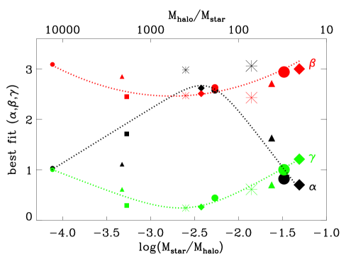
Figure 1: Best fit parameters for the inner slope, $\gamma$ (green), outer slope $\beta$ (red), and transition $\alpha$ (black) plotted as a function of integrated star formation efficiency, $M_{\star}$/$M_{\rm halo}$. The upper x-axis shows the corresponding $M_{\rm halo}$/$M_{\star}$ as a reference to the mass to light ratio. The parameters are for the double power law model of the dark matter density profile in Eq. (1). Each SPH simulated galaxy is represented by a symbol of a different size and shape as described in Table 1. The dotted lines represent the dependence of $\alpha$, $\beta$ and $\gamma$ on $M_{\star}$/$M_{\rm halo}$. Their functional forms are given in Eq. (3).

Fig. 1 shows how the inner slope $\gamma$ (green), the outer slope $\beta$ (red) and the transition parameter $\alpha$ (black) vary as a function of the $M_{\star}$/$M_{\rm halo}$ ratio. The symbols, as explained in Table 1, correspond to different initial conditions, while their sizes indicate the mass of the halo. The dotted lines show the best fit for each parameter, which we explain below in Eq. (3).

At very low integrated star formation efficiency, we expect to find the same profile as a dark matter only simulation since star formation is too sporadic to flatten the profile. Indeed, at $\log_{10}({{M_{\star}}}/{{M_{\rm halo}}})$$=$$-4.11$ the best fit values are $\alpha$=1, $\beta$=3, and $\gamma$=1, exactly an NFW halo.

At higher integrated star formation efficiencies, both the inner ($\gamma$) and outer ($\beta$) profile slopes decline to lower values than an NFW model, indicating halo expansion. At the same mass, the transition between inner and outer region becomes sharper: $\alpha$ increases as high as 3. Thus, while baryonic processes affect the profiles mainly in the inner region of slope $\gamma$, we must take their effects into account when deriving the other parameters $\alpha$ and $\beta$.

The star formation efficiency at which the cusp/core transition happens in our simulations is in agreement with the analytic calculation of Peñarrubia et al. (2012), who compared the energy needed to remove a cusp with the energy liberated by SNeII explosions.

The value of the inner slope ($\gamma$) varies with integrated star formation efficiency as found in Di Cintio et al. (2014). The minimum inner slope is at $-2.6$$<$$\log_{10}({{M_{\star}}}/{{M_{\rm halo}}})$$<$$-2.4$. So, as in Di Cintio et al. (2014), the dark matter cusps are most efficiently flattened when ${{M_{\star}}}/{{M_{\rm halo}}}\sim 3-5\times 10^{-3}$. Above $\log_{10}({{M_{\star}}}/{{M_{\rm halo}}})$$=$$-2.4$ (M/L$\sim$$250$), the parameters turn back towards the NFW values since more mass collapses to the centre than the energy from gas can pull around.

We fit the correlation between $\alpha$, $\beta$, $\gamma$ and the integrated star formation efficiency using two simple functions. The outer slope, $\beta$, is fit with a parabola as a function of $M_{\star}$/$M_{\rm halo}$. The inner slope, $\gamma$, and the transition parameter, $\alpha$, are both fit using a double power law model as a function of $M_{\star}$/$M_{\rm halo}$ as in Di Cintio et al. (2014). The best fit are shown as dotted lines in Figure 1. Their functional forms are:

$$\alpha=2.94-\log_{10}[(10^{X+2.33})^{-1.08}+(10^{X+2.33})^{2.29}]$$ (3)

$$\beta=4.23+1.34X+0.26X^{2}$$

$$\gamma=-0.06+\log_{10}[(10^{X+2.56})^{-0.68}+(10^{X+2.56})]$$

where $X=\log_{10}({{M_{\star}}}/{{M_{\rm halo}}})$.

Eq. (3) allows us to compute the entire dark matter profiles based solely on the stellar-to-halo mass ratio of a galaxy. We stress that the mass range of validity of Eq. (3) is $-4.1<\log_{10}({{M_{\star}}}/{{M_{\rm halo}}})<-1.3$: at lower masses the ($\alpha,\beta,\gamma$) value returns to the usual (1,3,1), NFW prediction, while at masses higher than $10^{12}M_{\odot}$, i.e. the Milky Way, other effects such as AGN feedback can concur to modify the profile in a way not currently testable with our set of simulations. In the future, having a larger statistical sample of simulated galaxies would certainly be desirable in order to compute the scatter in the relations defined by Eq. (3).

3.3 Checking the $\alpha,\beta,\gamma$ constraints

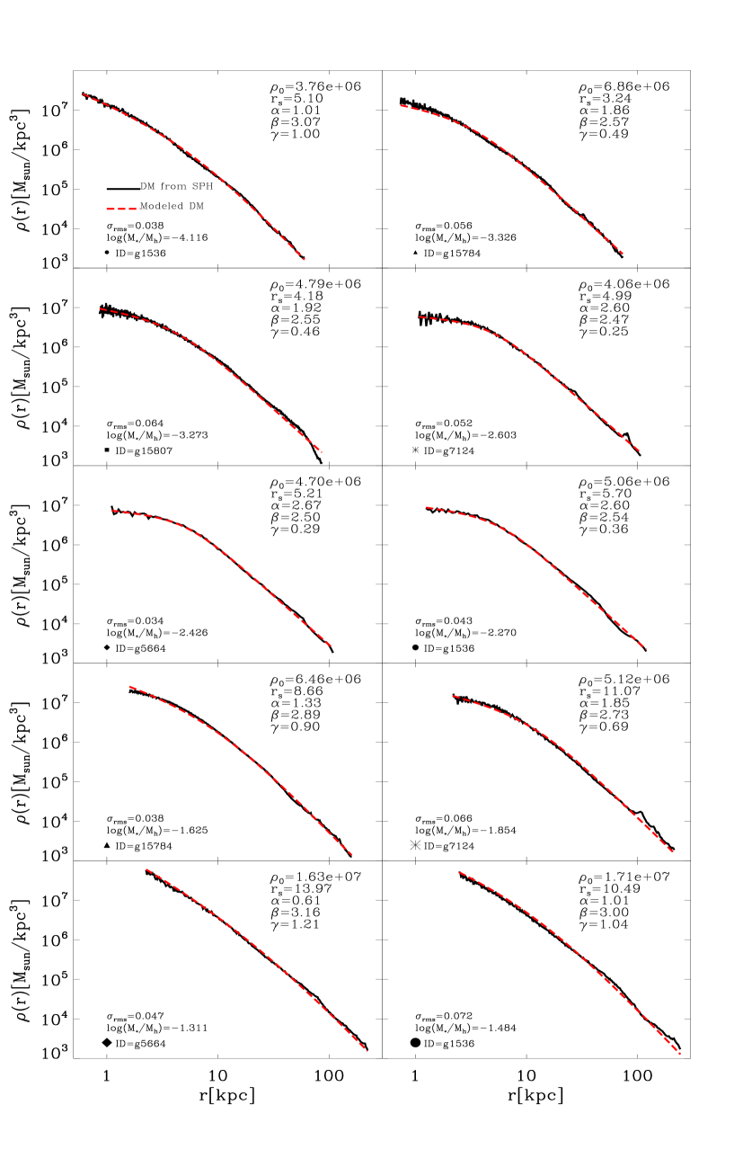
Figure 2: Halo dark matter density profiles (black line) and best fit model (dashed red line) for the hydrodynamically simulated galaxies. The profiles start at $0.01{{R_{\rm vir}}}$ to ensure convergence and the galaxies are shown in increasing halo mass order, same as in Table 1. The constrained $\alpha$, $\beta$ and $\gamma$ values, from Eq. (3), are shown together with the corresponding efficiency $M_{\star}$/$M_{\rm halo}$. The two free parameters of the fit, ${{r_{\rm s}}}$ and ${{\rho_{\rm s}}}$, are also listed as well as the r.m.s value of the fit $\sigma_{rms}$.

Using the constrained values for ($\alpha$, $\beta$, $\gamma$) from Eq. (3), we re-fit the dark matter density profiles of our haloes with the only standard two-free parameters, ${{r_{\rm s}}}$ and ${{\rho_{\rm s}}}$. The fit results are shown as dashed red lines in Fig. 2, superimposed on the dark matter density profiles of each hydrodynamically simulated galaxy (black lines). The galaxies are ordered according to their mass from top left to bottom right. The best fit values obtained for the scale radius ${{r_{\rm s}}}$ and scale density ${{\rho_{\rm s}}}$ are shown in the upper-right corner, along with the constrained values used for ($\alpha$, $\beta$, $\gamma$). The r.m.s. value of fit, defined as

$$\sigma_{rms}=\sqrt{\frac{1}{N_{\rm bins}}\sum_{k=1}^{N_{\rm bins}}(\rm log_{10}\rho_{sim,k}-log_{10}\rho_{fit,k})^{2}},$$ (4)

are shown in the lower-left corner. The average value of $\sigma_{rms}$ is 0.051 and shows that Eq. (3) can accurately describe the structure of simulated dark matter density profiles.

Since we started our analysis using a five-free parameters model, it is possible that some degeneracies may exist, and other combinations of ($\alpha,\beta,\gamma,{{r_{\rm s}}},\rho_{s}$) might be equally precise in describing dark matter haloes. We do not claim that our model is unique, but rather that provides a prescription that successfully describes very different dark matter profiles, both cored and cusp ones, in galaxies. Our model, reduced to a two-free parameters profile using the value of $M_{\star}$/$M_{\rm halo}$ (or simply $M_{\star}$) of each galaxy, shows very good precision in reproducing halo density profiles of cosmological hydrodynamically simulated galaxies of any halo mass.

3.4 Modeling rotation curves

It is may be easier to compare observations with the dark matter rotation curves, rather than with the density profile. We proceed by deriving the quantity $V_{\rm c}(r)=\sqrt{GM(r)/r}$ for the dark matter component within hydrodynamical simulations, where

$$M(r)=4\pi\rho_{s}\mathop{\text{\LARGE$\int_{\text{\normalsize$\scriptstyle\kern-1.75pt0$}}^{\text{\normalsize$\scriptstyle r$}}$}}\nolimits\frac{r^{\prime 2}}{\left(\frac{r^{\prime}}{{{r_{\rm s}}}}\right)^{\gamma}\left[1+\left(\frac{r^{\prime}}{{{r_{\rm s}}}}\right)^{\alpha}\right]^{(\beta-\gamma)/\alpha}}dr^{\prime}$$ (5)

The values ($\alpha,\beta,\gamma$) are constrained through Eq. (3) for each galaxy, while $\rho_{s}$ and ${{r_{\rm s}}}$ are the best-fit results as listed in Fig. 2, such that at the virial radius $M({{R_{\rm vir}}})$ equals $M_{\rm halo}$.

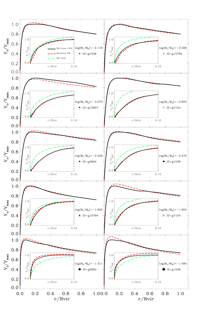
Figure 3: Circular velocity curves of dark matter within the galaxies used in this work, $V_{\rm c}(r)=\sqrt{GM(r)/r}$. The dark matter rotation curve from the SPH run is shown as solid black line, while our parametrized model for describing it is shown as red dashed line. The small insert within each plot shows a zoom-in of the region within $0.1{{R_{\rm vir}}}$, with the addition of the rotation curve from dark matter only run as dotted-dashed green line. The $V_{\rm c}$ of each galaxy is normalized to its maximum values $V_{\rm max}$, and plotted in units of ${{R_{\rm vir}}}$. From left to right, and top to bottom, galaxies are ordered as in Table 1.

The derived rotation curves for our model are shown as dashed red lines in Fig. 3, with galaxies again ordered by mass as in Fig. 2. The rotation curves taken directly from simulations, namely using the dark matter component within each hydrodynamically simulated galaxy, are shown as solid black lines. Each velocity curve is normalized to its maximum value $V_{max}$, and plotted in units of the virial radius.

The smaller panels within each plot show a zoom-in of $V_{c}(r)$ within $0.1{{R_{\rm vir}}}$, in order to better appreciate any difference between the actual simulations (solid black) and our parametrization (dashed red). Within this inner panel we also show as a green dotted-dashed line the rotation curve as derived from the dark matter only runs for each galaxy, scaled by the baryon fraction value. There is a very good agreement between our parametrized dark matter rotation curves and simulated ones, with differences that are below 10 per cent at any radii and for any galaxy. Further, when the contribution from the baryonic component is added to the rotation curves, the difference between the simulations and our parametrization will become even smaller, particularly at the high mass end of galaxy range where baryons dominate. By contrast, large differences can be seen between the rotation curves from dark matter only simulations (green dotted-dashed) and the rotation curves from the baryonic run (solid black) with the largest differences, as much as 50 per cent, being in intermediate mass galaxies. Such differences highlighting the error one would commit by modeling rotation curves of real galaxies using prediction from N-body simulations, with a NFW profile unmodified by baryonic processes. As opposite, our halo model introduces an error in the evaluation of galaxies’ rotation curves which is well within observational errors, and can therefore safely be applied to model dark matter haloes within real galaxies.

3.5 Constraining the concentration parameter

Now that we have demonstrated the precision of our density profile based on the stellar-to-halo mass ratio as in Eq. (3), we examine how one of the free parameters, the scale radius ${{r_{\rm s}}}$, varies as a function of integrated star forming efficiency, so that it could be implemented in semi-analytic models of galaxy formation. The concentration parameter of our hydrodynamically simulated galaxies does not always behave the same as in a corresponding dark matter only run.

First, as $\alpha$, $\beta$ and $\gamma$ vary, the definition of ${{r_{\rm s}}}$ changes. For consistency, Eq. (2) defines a conversion from ${{r_{\rm s}}}$ to $r_{-2}$, the radius at which the logarithmic slope of the profile equals $-2$. We define ${{c_{\rm SPH}}}\equiv{{R_{\rm vir}}}/r_{-2}$ as the concentration from the hydrodynamical simulation, and compare it with ${{c_{\rm DM}}}$, the NFW concentration from the dark matter only simulation.

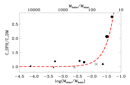
Figure 4: Ratio between concentration parameter $c={{R_{\rm vir}}}/r_{-2}$ in the SPH run and dark matter only run for our set of galaxies, as a function of $M_{\star}$/$M_{\rm halo}$. The upper x-axis shows the corresponding $M_{\rm halo}$/$M_{\star}$ as a reference to the mass to light ratio. ${{c_{\rm DM}}}$ has been derived fitting a NFW profile to the dark matter only version of each galaxy, while ${{c_{\rm SPH}}}$ has been computed applying our model profile to the dark matter halo of the galaxies in the hydrodynamical run, and converting the corresponding ${{r_{\rm s}}}$ into $r_{-2}$. The dashed red line represent the best model for the ${{c_{\rm SPH}}}/{{c_{\rm DM}}}$ values.

Fig. 4 shows the ratio between the concentration parameter in the hydrodynamical simulation and the dark matter only one, and how this ratio varies as a function of $M_{\star}$/$M_{\rm halo}$. Each simulation is represented by its symbol and size as described in Table 1. The dependence of ${{c_{\rm SPH}}}/{{c_{\rm DM}}}$ on $M_{\star}$/$M_{\rm halo}$ is nearly exponential. The best fit is:

$${{c_{\rm SPH}}}/{{c_{\rm DM}}}=1.0+0.00003e^{3.4X}$$ (6)

where $X=\log_{10}({{M_{\star}}}/{{M_{\rm halo}}})+4.5$.

Up to a mass ratio of $\log_{10}({{M_{\star}}}/{{M_{\rm halo}}})\sim-1.5$ (which corresponds to a halo mass of $10^{12}{{{\rm M}_{\odot}}}$), ${{c_{\rm SPH}}}$ is essentially the same as ${{c_{\rm DM}}}$. Thus, despite of the variation of the inner slope, the transition to the outer slope happens at the same radius $r_{-2}$ as in the dark matter only simulation.

Above $\log_{10}({{M_{\star}}}/{{M_{\rm halo}}})\sim-1.5$, instead, the difference is striking and the haloes become much more concentrated in the SPH case than the corresponding DM only run. In galaxies about the mass of the Milky Way, the inner region of the dark matter halo becomes smaller in our model, a signature of adiabatic contraction. Indeed, as shown already in Di Cintio et al. (2014), the increasing amount of stars at the centre of high mass spirals opposes the flattening effect of gas outflows generating instead a profile which is increasingly cuspy and more concentrated. Collisionless simulations in a WMAP3 cosmology find that the typical concentration of a $10^{12}$ M_⊙ halo [$\log_{10}({{M_{\star}}}/{{M_{\rm halo}}})=-1.5$] is $c\approx 8.5$ (Macciò et al., 2008); in our model with effective stellar feedback, the inner region of the halo shrinks by a factor of $\sim 2$, giving a concentration parameter ${{c_{\rm SPH}}}$ that can be $2.0-2.5$ times higher than the original N-body prediction.

Observations of the Milky Way are best fit with an NFW halo with high concentration parameter $c\approx 18-20$ (Battaglia et al., 2005; Catena & Ullio, 2010; Deason et al., 2012; Nesti & Salucci, 2013). The data include halo tracers like globular clusters, satellite galaxies, and dynamical observables like blue horizontal branch stars, red giant stars and maser star forming regions used to constrain the Galactic potential. While such a high value of the concentration $c$ is at odds with respect to N-body predictions, our study suggests that the mismatch could be related to the effect of infalling baryons, and that a value of $c$ compatible with the above mentioned works it is indeed expected once such effect is properly taken into account in simulations. Finally, a high concentration could arise possible tensions with the Tully-Fisher relation (Dutton et al., 2011) and the Fundamental Plane (Dutton et al., 2013) for high mass spirals, but this issue has to be explored in more detail once other effects relevant at L^∗ scales, such as feedback from AGN, will be included in the simulations.

4 Conclusions

It is well established that baryons affect dark matter density profiles of haloes in galaxies (e.g. Blumenthal et al., 1986; Navarro et al., 1996; El-Zant et al., 2001; Gnedin et al., 2004; Read & Gilmore, 2005; Goerdt et al., 2006; Read et al., 2006; Mashchenko et al., 2006; Tonini et al., 2006; Romano-Díaz et al., 2008; Del Popolo, 2009; Governato et al., 2010; Goerdt et al., 2010; Di Cintio et al., 2011; Zolotov et al., 2012; Governato et al., 2012; Macciò et al., 2012; Martizzi et al., 2013; Teyssier et al., 2013). Simple arguments compare the energy available from star formation with the depth of a galactic potential to estimate the degree of the change in the initial dark matter distribution (Peñarrubia et al., 2012; Pontzen & Governato, 2012, 2014).

This study describes the dark matter profiles of haloes from a suite of hydrodynamical cosmological galaxy formation simulations that include the effects of stellar feedback. The profiles are modeled using a generic double power law function. We find that the slope parameters of such model ($\alpha,\beta,\gamma$) vary in a systematic manner as a function of the ratio between $M_{\star}$/$M_{\rm halo}$, which we call integrated star formation efficiency. Using these fits allows us to propose a star formation efficiency dependent density profile for dark matter haloes that can be used for modeling observed galaxies and in semi-analytic models of galaxy formation.

The star formation efficiency dependent density profile has the form of a double power-law, with inner slope ($\gamma$), outer slope ($\beta$) and sharpness of transition ($\alpha$) fully determined by the stellar to halo mass ratio as given in Eq. 3. Thus, the five free parameters of the generic model reduce to two, the scale radius ${{r_{\rm s}}}$ and scale density ${{\rho_{\rm s}}}$, the same free parameters of the commonly used NFW model.

To examine how the scale radii varies as a function of integrated star formation efficiency, we compare the concentration parameter, $c={{R_{\rm vir}}}/r_{-2}$, of the dark matter haloes from galaxies simulated with hydrodynamics prescriptions to those from the corresponding dark matter only simulations. For masses below roughly the Milky Way’s the concentrations are similar, indicating that while the profiles may be significantly different from NFW, particularly in terms of inner slope, the radius at which the logarithmic slope of the profile equals -2 is the same as in the NFW model, indicating no net halo response at scales near the scale radius.

However, for Milky Way mass galaxies the haloes from the hydro runs become as much as two times more concentrated than in the pure dark matter runs. Such high concentrations are consistent to what has been derived from observations of Milky Way’s dynamical tracers (Battaglia et al., 2005; Catena & Ullio, 2010; Deason et al., 2012; Nesti & Salucci, 2013).

Thus, specifying the halo or stellar mass for a galaxy is sufficient to completely describe the shape of dark matter profiles for galaxies ranging in mass from dwarfs to L^∗, based on the influence of stellar feedback. Importantly, the simulations we utilize in determining these profiles match a wide range of scaling relations Brook et al. (2012), meaning that their radial mass distributions are well constrained.

The main features of the mass dependent dark matter profile are:

• Baryons affect the profile shape parameters. For galaxies with flat inner profiles $\gamma$ the sharpness of transition parameter, $\alpha$, increases from 1 to 3 and corresponds to a small decrease in the slope of the outer profile $\beta$.

• At low integrated star formation efficiencies, ${{M_{\star}}}/{{M_{\rm halo}}}\lower 2.15277pt\hbox{$\;\buildrel<\over{\sim}\;$}10^{-4}$ (galaxies with ${{M_{\star}}}\lower 2.15277pt\hbox{$\;\buildrel<\over{\sim}\;$}5$x$10^{6}{{{\rm M}_{\odot}}}$), dark matter haloes maintain the usual NFW profile as in dark matter only simulations.

• At higher efficiencies the profile becomes progressively flatter. The most cored galaxies are found at ${{M_{\star}}}/{{M_{\rm halo}}}\approx 3-5\times 10^{-3}$ or $M_{\star}$ $\sim$$10^{8.5}$${\rm M}_{\odot}$.

• Galaxies with ${{M_{\star}}}/{{M_{\rm halo}}}\mathrel{\hbox{\hbox to0.0pt{\hbox{\lower 4.0pt\hbox{$\sim$}}\hss}\hbox{$>$}}}5\times 10^{-3}$ (${{M_{\star}}}\mathrel{\hbox{\hbox to0.0pt{\hbox{\lower 4.0pt\hbox{$\sim$}}\hss}\hbox{$>$}}}10^{8.5}{{{\rm M}_{\odot}}}$), become progressively steeper in the inner region as their mass increases.

• The parameters ($\alpha,\beta,\gamma$) returns to the NFW values of (1,3,1) for L^∗ galaxies.

• However such L^∗ galaxies, and more in general galaxies with ${{M_{\star}}}/{{M_{\rm halo}}}\mathrel{\hbox{\hbox to0.0pt{\hbox{\lower 4.0pt\hbox{$\sim$}}\hss}\hbox{$>$}}}0.03$, are up to a factor of 2.5 more concentrated than the corresponding dark matter only simulations.

In an Appendix we show step-by-step how to derive the dark matter profile for any galaxy mass.

Our results show that baryonic effects substantially change the structure of cold dark matter haloes from those predicted from dissipationless simulations, and therefore must be taken into account in any model of galaxy formation.

Of course, our model uses a particular feedback implementation, namely thermal feedback in the form of blast-wave formalism. Yet Teyssier et al. (2013) finds a similar degree of core creation, at least in low mass galaxies, using a different feedback scheme. Both studies are based on the same mechanisms for core creation, i.e. rapid and repeated outflows of gas which result in changes in the potential. Indeed, the simulations closely follow the analytic model of core creation presented in Pontzen & Governato (2012), indicating that the precise details of the feedback implementation are not central to our results, at least not in a qualitative manner. Galaxy formation models which do not include impulsive supernova explosions driving outflows from the central regions will not form cores in this manner.

In a forthcoming paper we will present a comprehensive comparison of our predicted density profile with the inferred mass distribution of observed galaxies, with particular emphasis on Local Group members.

Appendix A Recipe to derive a mass dependent density profile

We summarize here the steps necessary to derive, for a given halo mass, the corresponding dark matter profile which takes into account the effects of baryons:

• Input the halo mass $M_{\rm halo}$ and the stellar mass $M_{\star}$ of a galaxy. In case that only one of these two quantities is known, use the abundance matching relation (Brook et al., 2014; Moster et al., 2013; Guo et al., 2011) to derive the second one.

• Specify an overdensity criterion, such that the halo mass is defined as the mass contained within a sphere of radius $R_{\rm vir}$ containing $\Delta$ times the critical density of the Universe $\rho_{\rm crit}=3H^{2}/8\pi G$:

  $${{M_{\rm halo}}}=\frac{4}{3}\pi R_{vir}^{3}\Delta\rho_{crit}$$ (7)

  Common choices of $\Delta$ are $\Delta_{\rm 200}=200$ or $\Delta_{\rm vir}=18\pi^{2}+82x-39x^{2}$ with $x=\Omega_{m}-1$ at $z=0$ (Bryan & Norman, 1998). In a WMAP3 cosmology $\Delta_{\rm vir}=92.8$.

• Compute the halo profile parameters $(\alpha,\beta,\gamma)$ as a function of integrated star formation efficiency $M_{\star}$/$M_{\rm halo}$ using Eq. (3). Recall that the range of validity of Eq. (3) is $-4.1<\log_{10}({{M_{\star}}}/{{M_{\rm halo}}})<-1.3$: at lower efficiencies the ($\alpha,\beta,\gamma$) value returns to the usual (1,3,1), NFW prediction.

• Obtain the concentration parameter ${{c_{\rm SPH}}}={{R_{\rm vir}}}/r_{-2}$ via Eq. (6), where the quantity $c_{\rm DM}$ is the typical concentration of a halo of mass $M_{\rm halo}$ coming from N-body simulations (Dutton & Macciò, 2014; Macciò et al., 2008). In this way we have derived the $r_{-2}$ at which the logarithmic slope of the profile equals -2.

• Convert such $r_{-2}$ into the corresponding scale radius $r_{\rm s}$  using Eq. (2). This is the scale radius that enters into Eq. (1).

• Find the scale density $\rho_{\rm s}$ by imposing the normalization $M(<R_{vir})={{M_{\rm halo}}}$:

  $$\rho_{s}={{M_{\rm halo}}}/4\pi\mathop{\text{\LARGE$\int_{\text{\normalsize$\scriptstyle\kern-1.75pt0$}}^{\text{\normalsize$\scriptstyle R_{vir}$}}$}}\nolimits\frac{r^{2}}{\left(\frac{r}{{{r_{\rm s}}}}\right)^{\gamma}\left[1+\left(\frac{r}{{{r_{\rm s}}}}\right)^{\alpha}\right]^{(\beta-\gamma)/\alpha}}dr$$ (8)

• The mass dependent density profile can now be obtained through Eq. (1) and the corresponding circular velocity via $V_{\rm c}(r)=\sqrt{GM(r)/r}$.

• In case of fitting observed rotation curves of galaxies the scale radius $r_{\rm s}$ and scale density $\rho_{\rm s}$ should be left as the two free parameters of the model.

References

- Agertz et al. (2007) Agertz O., Moore B., Stadel J., Potter D., Miniati F., Read J., Mayer L., Gawryszczak A., Kravtsov A., Nordlund Å., Pearce F., Quilis V., Rudd D., Springel V., Stone J., Tasker E., Teyssier R., Wadsley J., Walder R., 2007, MNRAS, 380, 963
- Battaglia et al. (2005) Battaglia G., Helmi A., Morrison H., Harding P., Olszewski E. W., Mateo M., Freeman K. C., Norris J., Shectman S. A., 2005, MNRAS, 364, 433
- Blumenthal et al. (1986) Blumenthal G. R., Faber S. M., Flores R., Primack J. R., 1986, ApJ, 301, 27
- Brook et al. (2014) Brook C. B., Di Cintio A., Knebe A., Gottlöber S., Hoffman Y., Yepes G., Garrison-Kimmel S., 2014, ApJ, 784, L14
- Brook et al. (2011) Brook C. B., Governato F., Roškar R., Stinson G., Brooks A. M., Wadsley J., Quinn T., Gibson B. K., Snaith O., Pilkington K., House E., Pontzen A., 2011, MNRAS, pp 595–+
- Brook et al. (2012) Brook C. B., Stinson G., Gibson B. K., Roškar R., Wadsley J., Quinn T., 2012, MNRAS, 419, 771
- Brook et al. (2012) Brook C. B., Stinson G., Gibson B. K., Wadsley J., Quinn T., 2012, MNRAS, 424, 1275
- Bryan & Norman (1998) Bryan G. L., Norman M. L., 1998, ApJ, 495, 80
- Bullock et al. (2001) Bullock J. S., Kolatt T. S., Sigad Y., Somerville R. S., Kravtsov A. V., Klypin A. A., Primack J. R., Dekel A., 2001, MNRAS, 321, 559
- Catena & Ullio (2010) Catena R., Ullio P., 2010, Journal of Cosmology and Astro-Particle Physics, 8, 4
- Chabrier (2003) Chabrier G., 2003, ApJL, 586, L133
- Cole et al. (2011) Cole D. R., Dehnen W., Wilkinson M. I., 2011, MNRAS, 416, 1118
- de Blok et al. (2001) de Blok W. J. G., McGaugh S. S., Bosma A., Rubin V. C., 2001, ApJ, 552, L23
- de Blok et al. (2008) de Blok W. J. G., Walter F., Brinks E., Trachternach C., Oh S.-H., Kennicutt Jr. R. C., 2008, AJ, 136, 2648
- Deason et al. (2012) Deason A. J., Belokurov V., Evans N. W., An J., 2012, MNRAS, 424, L44
- Del Popolo (2009) Del Popolo A., 2009, ApJ, 698, 2093
- Del Popolo (2010) Del Popolo A., 2010, MNRAS, 408, 1808
- Di Cintio et al. (2014) Di Cintio A., Brook C. B., Macciò A. V., Stinson G. S., Knebe A., Dutton A. A., Wadsley J., 2014, MNRAS, 437, 415
- Di Cintio et al. (2011) Di Cintio A., Knebe A., Libeskind N. I., Yepes G., Gottlöber S., Hoffman Y., 2011, MNRAS, 417, L74
- Duffy et al. (2010) Duffy A. R., Schaye J., Kay S. T., Dalla Vecchia C., Battye R. A., Booth C. M., 2010, MNRAS, 405, 2161
- Dutton et al. (2011) Dutton A. A., Conroy C., van den Bosch F. C., Simard L., Mendel J. T., Courteau S., Dekel A., More S., Prada F., 2011, MNRAS, 416, 322
- Dutton & Macciò (2014) Dutton A. A., Macciò A. V., 2014, ArXiv e-prints,1402.7073
- Dutton et al. (2013) Dutton A. A., Macciò A. V., Mendel J. T., Simard L., 2013, MNRAS, 432, 2496
- Dutton et al. (2007) Dutton A. A., van den Bosch F. C., Dekel A., Courteau S., 2007, ApJ, 654, 27
- El-Zant et al. (2001) El-Zant A., Shlosman I., Hoffman Y., 2001, ApJ, 560, 636
- Freyer et al. (2006) Freyer T., Hensler G., Yorke H. W., 2006, ApJ, 638, 262
- Gao et al. (2008) Gao L., Navarro J. F., Cole S., Frenk C. S., White S. D. M., Springel V., Jenkins A., Neto A. F., 2008, MNRAS, 387, 536
- Gill et al. (2004) Gill S. P. D., Knebe A., Gibson B. K., 2004, MNRAS, 351, 399
- Gnedin et al. (2004) Gnedin O. Y., Kravtsov A. V., Klypin A. A., Nagai D., 2004, ApJ, 616, 16
- Goerdt et al. (2010) Goerdt T., Moore B., Read J. I., Stadel J., 2010, ApJ, 725, 1707
- Goerdt et al. (2006) Goerdt T., Moore B., Read J. I., Stadel J., Zemp M., 2006, MNRAS, 368, 1073
- Governato et al. (2010) Governato F., Brook C., Mayer L., Brooks A., Rhee G., Wadsley J., Jonsson P., Willman B., Stinson G., Quinn T., Madau P., 2010, Nature, 463, 203
- Governato et al. (2012) Governato F., Zolotov A., Pontzen A., Christensen C., Oh S. H., Brooks A. M., Quinn T., Shen S., Wadsley J., 2012, MNRAS, 422, 1231
- Guo et al. (2011) Guo Q., Cole S., Eke V., Frenk C., 2011, MNRAS, 417, 370
- Guo et al. (2010) Guo Q., White S., Li C., Boylan-Kolchin M., 2010, MNRAS, 404, 1111
- Hernquist (1990) Hernquist L., 1990, ApJ, 356, 359
- Jaffe (1983) Jaffe W., 1983, MNRAS, 202, 995
- Kannan et al. (2012) Kannan R., Macciò A. V., Pasquali A., Moster B. P., Walter F., 2012, ApJ, 746, 10
- Kannan et al. (2014) Kannan R., Stinson G. S., Macciò A. V., Brook C., Weinmann S. M., Wadsley J., Couchman H. M. P., 2014, MNRAS, 437, 3529
- Katz (1992) Katz N., 1992, ApJ, 391, 502
- Kay et al. (2002) Kay S. T., Pearce F. R., Frenk C. S., Jenkins A., 2002, MNRAS, 330, 113
- Kennicutt (1998) Kennicutt R. C., 1998, ApJ, 498, 541
- Knollmann & Knebe (2009) Knollmann S. R., Knebe A., 2009, ApJS, 182, 608
- Kuzio de Naray et al. (2008) Kuzio de Naray R., McGaugh S. S., de Blok W. J. G., 2008, ApJ, 676, 920
- Kuzio de Naray et al. (2009) Kuzio de Naray R., McGaugh S. S., Mihos J. C., 2009, ApJ, 692, 1321
- Macciò et al. (2008) Macciò A. V., Dutton A. A., van den Bosch F. C., 2008, MNRAS, 391, 1940
- Macciò et al. (2007) Macciò A. V., Dutton A. A., van den Bosch F. C., Moore B., Potter D., Stadel J., 2007, MNRAS, 378, 55
- Macciò et al. (2012) Macciò A. V., Stinson G., Brook C. B., Wadsley J., Couchman H. M. P., Shen S., Gibson B. K., Quinn T., 2012, ApJL, 744, L9
- Martizzi et al. (2013) Martizzi D., Teyssier R., Moore B., 2013, MNRAS, 432, 1947
- Mashchenko et al. (2006) Mashchenko S., Couchman H. M. P., Wadsley J., 2006, Nature, 442, 539
- Merritt et al. (2006) Merritt D., Graham A. W., Moore B., Diemand J., Terzić B., 2006, AJ, 132, 2685
- Mo & Mao (2004) Mo H. J., Mao S., 2004, MNRAS, 353, 829
- Moore (1994) Moore B., 1994, Nature, 370, 629
- Moster et al. (2013) Moster B. P., Naab T., White S. D. M., 2013, MNRAS, 428, 3121
- Moster et al. (2010) Moster B. P., Somerville R. S., Maulbetsch C., van den Bosch F. C., Macciò A. V., Naab T., Oser L., 2010, ApJ, 710, 903
- Muñoz-Cuartas et al. (2011) Muñoz-Cuartas J. C., Macciò A. V., Gottlöber S., Dutton A. A., 2011, MNRAS, 411, 584
- Navarro et al. (1996) Navarro J. F., Eke V. R., Frenk C. S., 1996, MNRAS, 283, L72
- Navarro et al. (1996) Navarro J. F., Frenk C. S., White S. D. M., 1996, ApJ, 462, 563
- Navarro et al. (2004) Navarro J. F., Hayashi E., Power C., Jenkins A. . R., Frenk C. S., White S. D. M., Springel V., Stadel J., Quinn T. R., 2004, MNRAS, 349, 1039
- Navarro et al. (2010) Navarro J. F., Ludlow A., Springel V., Wang J., Vogelsberger M., White S. D. M., Jenkins A., Frenk C. S., Helmi A., 2010, MNRAS, 402, 21
- Nesti & Salucci (2013) Nesti F., Salucci P., 2013, Journal of Cosmology and Astro-Particle Physics, 7, 16
- Obreja et al. (2014) Obreja A., Brook C. B., Stinson G., Domínguez-Tenreiro R., Gibson B. K., Silva L., Granato G. L., 2014, ArXiv e-prints,1404.0043
- Oh et al. (2011) Oh S.-H., de Blok W. J. G., Brinks E., Walter F., Kennicutt Jr. R. C., 2011, AJ, 141, 193
- Peñarrubia et al. (2012) Peñarrubia J., Pontzen A., Walker M. G., Koposov S. E., 2012, ApJ, 759, L42
- Pontzen & Governato (2012) Pontzen A., Governato F., 2012, MNRAS, 421, 3464
- Pontzen & Governato (2014) Pontzen A., Governato F., 2014, Nature, 506, 171
- Power et al. (2003) Power C., Navarro J. F., Jenkins A., Frenk C. S., White S. D. M., Springel V., Stadel J., Quinn T., 2003, MNRAS, 338, 14
- Prada et al. (2012) Prada F., Klypin A. A., Cuesta A. J., Betancort-Rijo J. E., Primack J., 2012, MNRAS, 423, 3018
- Read & Gilmore (2005) Read J. I., Gilmore G., 2005, MNRAS, 356, 107
- Read et al. (2006) Read J. I., Goerdt T., Moore B., Pontzen A. P., Stadel J., Lake G., 2006, MNRAS, 373, 1451
- Romano-Díaz et al. (2008) Romano-Díaz E., Shlosman I., Hoffman Y., Heller C., 2008, ApJ, 685, L105
- Salucci & Burkert (2000) Salucci P., Burkert A., 2000, ApJ, 537, L9
- Schmidt (1959) Schmidt M., 1959, ApJ, 129, 243
- Shen et al. (2010) Shen S., Wadsley J., Stinson G., 2010, MNRAS, 407, 1581
- Simon et al. (2005) Simon J. D., Bolatto A. D., Leroy A., Blitz L., Gates E. L., 2005, ApJ, 621, 757
- Spergel et al. (2007) Spergel et al. D. N., 2007, ApJS, 170, 377
- Springel et al. (2008) Springel V., Wang J., Vogelsberger M., Ludlow A., Jenkins A., Helmi A., Navarro J. F., Frenk C. S., White S. D. M., 2008, MNRAS, 391, 1685
- Stinson et al. (2006) Stinson G., Seth A., Katz N., Wadsley J., Governato F., Quinn T., 2006, MNRAS, 373, 1074
- Stinson et al. (2010) Stinson G. S., Bailin J., Couchman H., Wadsley J., Shen S., Nickerson S., Brook C., Quinn T., 2010, MNRAS, 408, 812
- Stinson et al. (2013) Stinson G. S., Brook C., Macciò A. V., Wadsley J., Quinn T. R., Couchman H. M. P., 2013, MNRAS, 428, 129
- Teyssier et al. (2013) Teyssier R., Pontzen A., Dubois Y., Read J. I., 2013, MNRAS, 429, 3068
- Tonini et al. (2006) Tonini C., Lapi A., Salucci P., 2006, ApJ, 649, 591
- Wadsley et al. (2004) Wadsley J. W., Stadel J., Quinn T., 2004, New Astronomy, 9, 137
- Walker & Peñarrubia (2011) Walker M. G., Peñarrubia J., 2011, ApJ, 742, 20
- Zolotov et al. (2012) Zolotov A., Brooks A. M., Willman B., Governato F., Pontzen A., Christensen C., Dekel A., Quinn T., Shen S., Wadsley J., 2012, ApJ, 761, 71