A Semi-Lagrangian scheme for a degenerate second order Mean Field Game system

Abstract

In this paper we study a fully discrete Semi-Lagrangian approximation of a second order Mean Field Game system, which can be degenerate. We prove that the resulting scheme is well posed and, if the state dimension is equals to one, we prove a convergence result. Some numerical simulations are provided, evidencing the convergence of the approximation and also the difference between the numerical results for the degenerate and non-degenerate cases.

Keywords: Mean field games, Degenerate second order system, Semi-Lagrangian schemes, Nu-merical methods.

MSC 2000: Primary: 65M12, 91A13; Secondary: 65M25, 91A23, 49J15, 35F21, 35Q84 .

1 Introduction

Mean Field Games (MFG) systems were introduced independently by [22, 23] and [25, 26, 27] in order to model dynamic games with a large number of indistinguishable small players. In the model proposed in [26, 27] the asymptotic equilibrium is described by means of a system of two Partial Differential Equations (PDEs). The first equation, together with a final condition, is a Hamilton-Jacobi-Bellman (HJB) equation describing the value function of an average player whose cost function depends on the distribution $m$ of the entire population. The second equation is a Fokker-Planck equation which, together with an initial distribution $m_{0}$, describes the fact that $m$ evolves following the optimal dynamics of the average player. We refer the reader to the original papers [22, 23, 25, 26, 27] and the surveys [10, 19] for a detailed description of the problem and to [21] for some interesting applications.

Numerical methods to solve MFGs problems have been addressed by several authors. Let us mention the papers [3, 24, 20, 2, 11] where the second order system (i.e. when the underlying dynamics is stochastic) is treated and to [9, 12] for the first order case (i.e. when the underlying dynamics is deterministic).

In this article we consider the following second order possibly degenerated MFG system

$$\begin{array}[]{rcl}-\partial_{t}v-\mbox{$\frac{1}{2}$}\mbox{tr}\left(\sigma(t)\sigma(t)^{\top}D^{2}v\right)+\mbox{$\frac{1}{2}$}|Dv|^{2}&=&F(x,m(t))\;\;\hbox{in }\mathbb{R}^{d}\times]0,T[,\\[6.0pt] \partial_{t}m-\mbox{$\frac{1}{2}$}\mbox{tr}\left(\sigma(t)\sigma(t)^{\top}D^{2}v\right)-\mbox{div}\big{(}Dvm\big{)}&=&0\;\;\;\hbox{in }\mathbb{R}^{d}\times]0,T[,\\[6.0pt] v(x,T)=G(x,m(T))\;\;\mbox{for }x\in\mathbb{R}^{d},&&\;\;m(\cdot,0)=m_{0}(\cdot)~\in\mathcal{P}_{1}(\mathbb{R}^{d}),\end{array}$$ (1.1)

where $\mathcal{P}_{1}(\mathbb{R}^{d})$ is the set of probability measures over $\mathbb{R}^{d}$ having finite first order moment, $\sigma:[0,T]\to\mathbb{R}^{d\times r}$ and $F$, $G:\mathbb{R}^{d}\times\mathcal{P}_{1}\to\mathbb{R}$ are two functions satisfying some assumptions described in Section 2. Up to the best of our knowledge, for this system, existence and uniqueness results have not been established yet (except for the case $r=d$, $\sigma:=\hat{\sigma}\mathbb{I}_{d\times d}$, $\hat{\sigma}\in\mathbb{R}$).

The aim of this work is to provide a fully-discrete Semi-Lagrangian discretization of (1.1), to study the main properties of the scheme and to establish a convergence result for the solutions of the discrete system. The line of argument is similar to the one analyzed in [12]. Given a continuous measure-valued application $\mu(\cdot)$ and a space-time step $(\rho,h)$ we discretize the HJB

$$\begin{array}[]{rcl}-\partial_{t}v-\mbox{$\frac{1}{2}$}\mbox{tr}\left(\sigma(t)\sigma(t)^{\top}D^{2}v\right)+\mbox{$\frac{1}{2}$}|Dv|^{2}&=&F(x,\mu(t))\;\;\hbox{in }Q,\\[6.0pt] v(x,T)&=&G(x,\mu(T))\;\;\mbox{for }x\in\mathbb{R}^{d},\end{array}$$ (1.2)

using a fully-discrete Semi-Lagrangian scheme in the spirit of [8, 16]. We then regularize the solution of the scheme by convolution with a mollifier $\phi_{\varepsilon}$ ($\varepsilon>0$). The resulting function is called $v^{\varepsilon}_{\rho,h}[\mu]$. In order to discretize the second equation we propose a natural extension to the second order case of the scheme in [12] designed for the first order equation (i.e. with $\sigma=0$). The solution of the scheme is denoted by $m^{\varepsilon}_{\rho,h}[\mu](\cdot)$. The fully-discretization of problem (1.1) is thus to find $\mu(\cdot)$ such that $m^{\varepsilon}_{\rho,h}[\mu](\cdot)=\mu(\cdot)$. The existence of a solution of the discrete problem is established in Theorem 5.1 by standard arguments based on the Brouwer fixed point Theorem. The convergence of the solutions of the discrete system to a solution of (1.1) is much more delicate. As a matter of fact, as in [12] we establish in Theorem 5.2 the convergence result only when the state dimension $d$ is equals to one. Under suitable conditions over the discretization parameters, the proof is based on three crucial results. The first one is a relative compactness property for $m^{\varepsilon}_{\rho,h}[\mu](\cdot)$, which can be obtained as a consequence of a Markov chain interpretation of the scheme. The second result is the discrete semiconcavity of $v^{\varepsilon}_{\rho,h}[\mu]$ (see e.g. [1]), which implies a.e. convergence of $Dv^{\varepsilon}_{\rho,h}[\mu]$ to $Dv[\mu]$ (where $v[\mu]$ is the unique viscosity solution of (1.2)). The third result are $L^{\infty}$-bounds for the density of $m^{\varepsilon}_{\rho,h}[\mu](\cdot)$, where the one dimensional assumption plays an important role. We remark that our convergence result proves the existence of a solution of (1.1) when $d=1$. Moreover, our results are valid for more general Hamiltionians, as the ones considered in [1] (see Remark 5.1(ii)). However, since the proofs are already rather technical, as in [12], we preferred to present the details for the quadratic Hamiltonian case.

The paper is organized as follows. In Section 2 we fix some notations and we state our main assumptions. In Section 3 we provide the natural Semi-Lagrangian discretization for the HJB equation and we prove its main properties. In Section 4 we propose a scheme for the Fokker-Planck equation and we prove that the associated solutions, as functions of the discretization parameters, form a relatively compact set. In Section 5 we prove our main results, the existence of a solution of the discrete system and, if $d=r=1$, the convergence to a solution of (1.1). Finally, in Section 6 we present some numerical simulations showing the difference between the numerical approximation between degenerate and non-degenerate systems.

2 Preliminaries

Let us first fix some notations. For $x\in~\mathbb{R}^{d}$ we will denote by $|x|=\sqrt{x^{\top}x}$ for the usual Euclidean norm. In the entire article $c>0$ will be a generic constant, which can change from line to line. For $u\in\mathbb{R}^{d}\times[0,T]\to\mathbb{R}$ we will denote by $\partial_{t}u$ for the partial derivative of $u$ (if it exists) w.r.t. the time variable and by $Du$, $D^{2}u$ the gradient and Hessian of $u$ (if they exist) w.r.t. the space variables. We denote by $\mathcal{P}(\mathbb{R}^{d})$ the set of Borel probability measures $\mu$ over $\mathbb{R}^{d}$ and, for $p\in[1,\infty[$, we say that $\mu\in\mathcal{P}_{p}(\mathbb{R}^{d})$ if

$$\int_{\mathbb{R}^{d}}|x|^{p}{\rm d}\mu(x)<+\infty.$$

The distance $d_{p}~:\mathcal{P}_{p}(\mathbb{R}^{d})\times\mathcal{P}_{p}(\mathbb{R}^{d})\to\mathbb{R}$ is defined as

$$d_{p}(\mu_{1},\mu_{2}):=\inf_{\gamma\in\mathcal{P}(\mathbb{R}^{d}\times\mathbb{R}^{d})}\left\{\left[\int_{\mathbb{R}^{d}\times\mathbb{R}^{d}}|x-y|^{p}{\rm d}\gamma(x,y)\right]^{\frac{1}{p}}\;;\;\gamma(A\times\mathbb{R}^{d})=\mu_{1}(A),\;\;\gamma(\mathbb{R}^{d}\times B)=\mu_{2}(B)\;\;\forall\;A,B\in\mathcal{B}(\mathbb{R}^{d})\right\}.$$

It is well-known (see e.g. [29, Theorem 1.14]) that $d_{1}$, can be expressed in the following dual form

$$d_{1}(\mu_{1},\mu_{2})=\sup_{\phi}\left\{\int_{\mathbb{R}^{d}}\phi(x){\rm d}[\mu_{1}-\mu_{2}](x)\ ;\ \phi\;\mbox{is 1-Lipschitz}\right\}.$$ (2.1)

Let us recall the following useful result (see e.g. [4, Chapter 7] and [10, Lemma 5.7]):

Lemma 2.1

Let $q>p>0$ and $\mathcal{K}\subseteq\mathcal{P}_{p}(\mathbb{R}^{d})$ be such that

$$\sup_{\mu\in\mathcal{K}}\int_{\mathbb{R}^{d}}|x|^{q}{\rm d}\mu(x)<\infty.$$

Then $\mathcal{K}$ is a relatively compact set in $\mathcal{P}_{p}(\mathbb{R}^{d})$.

We assume now the following assumptions on the data of (1.1):
(A1) We suppose that:
(i) $F$ and $G$ are uniformly bounded over $\mathbb{R}^{d}\times\mathcal{P}_{1}$ and for every $m\in\mathcal{P}_{1}(\mathbb{R}^{d})$, the functions $F(\cdot,m)$, $G(\cdot,m)$ are $C^{2}$ and their first and second derivatives are bounded in $\mathbb{R}^{d}$, uniformly with respect to $m$, i.e. $\exists\;c>0$ such that

$$\|F(\cdot,m)\|_{C^{2}}+\|G(\cdot,m)\|_{C^{2}}\leq c\hskip 14.22636pt\forall\;m\in\mathcal{P}_{1}(\mathbb{R}^{d}),$$

where for $\phi:\mathbb{R}^{d}\to\mathbb{R}$ we set $\|\phi\|_{C^{2}}:=\sup_{x\in\mathbb{R}^{d},\;|\alpha|\leq 2}\left|D^{\alpha}\phi(x)\right|$.
(ii) Denoting by $\sigma_{\ell}:[0,T]\to\mathbb{R}^{d}$ ($\ell=1,\ldots,r$) the $\ell$ column vector of the matrix $\sigma$, we assume that $\sigma_{\ell}$ is continuous.
(iii) The measure $m_{0}$ is absolutely continuous, with density still denoted as $m_{0}$. Moreover, we suppose that $m_{0}$ is essentially bounded and has compact support, i.e. there exists $c>0$ such that $\mbox{supp}(m_{0})\subseteq B(0,c)$, where $B(0,c):=\{x\in\mathbb{R}^{d}\;;\;|x|<c\}$.

We say that $(v,m)$ is a solution of (1.1) if the first equation is satisfied in the viscosity sense (see e.g. [14, 18]), while the second one is satisfied in the distributional sense (see e.g [17]), i.e. for every $\phi\in\mathcal{C}_{c}^{\infty}\left(\mathbb{R}^{d}\right)$ and $t\in[0,T]$

$$\int_{\mathbb{R}}\phi(x){\rm d}m(t)(x)=\int_{\mathbb{R}}\phi(x){\rm d}m_{0}(x)+\int_{0}^{t}\int_{\mathbb{R}^{d}}\left[\mbox{$\frac{1}{2}$}\mbox{Tr}(\sigma\sigma^{\top}(s)D^{2}\phi(x))-\langle D\phi(x),Dv(x,s)\rangle\right]{\rm d}m(s)(x){\rm d}s.$$

Our aim in this work is to provide a discretization scheme for (1.1). Given $h,\rho>0$, let us define a space grid $\mathcal{G}_{\rho}$ and a time-space grid $\mathcal{G}_{\rho,h}$ as

$$\mathcal{G}_{\rho}:=\{x_{i}=i\rho,\;i\in\mathbb{Z}^{d}\},\hskip 22.76228pt\mathcal{G}_{\rho,h}:=\mathcal{G}_{\rho}\times\{t_{k}\}_{k=0}^{N},$$

where $t_{k}=kh$ ($k=0,\ldots,N$) and $t_{N}=Nh=T$. We call $B(\mathcal{G}_{\rho})$ and $B(\mathcal{G}_{\rho,h})$ the spaces of bounded functions defined respectively on $\mathcal{G}_{\rho}$ and $\mathcal{G}_{\rho,h}$. For $f\in B(\mathcal{G}_{\rho})$ and $g\in B(\mathcal{G}_{\rho,h})$ we set $f_{i}:=f(x_{i}),\,g_{i,k}:=g(x_{i},t_{k})$. Given a regular triangulation of $\mathbb{R}^{d}$ with vertices belonging to $\mathcal{G}_{\rho}$, we set $\beta_{i}(x)$ for the barycentric coordinate of $x$ relative to $x_{i}$ in the triangulation. Clearly $\beta_{i}(x)$ is a piecewise affine function with compact support, satisfying $0\leq\beta_{i}\leq 1$, $\beta_{i}(x_{j})=\delta_{ij}$ for all $x_{j}\in\mathcal{G}_{\rho}$ (the Kronecker symbol) and $\sum_{i\in\mathbb{Z}^{d}}\beta_{i}(x)=1$ for all $x\in\mathbb{R}^{d}$. We consider the following linear interpolation operator

$$I[f](\cdot):=\sum_{i\in\mathbb{Z}^{d}}f_{i}\beta_{i}(\cdot)\hskip 5.69046pt\mbox{for }f\in B(\mathcal{G}_{\rho}).$$ (2.2)

We recall two basic results about the interpolation operator $I$ (see e.g. [13, 28]). Given $\phi\in C_{b}(\mathbb{R}^{d})$ (the space of bounded continuous functions on $\mathbb{R}^{d}$), let us define $\hat{\phi}\in B(\mathcal{G}_{\rho})$ by $\hat{\phi}_{i}:=\phi(x_{i})$ for all $i\in\mathbb{Z}^{d}$. Suppose that $\phi:\mathbb{R}^{d}\to\mathbb{R}$ is Lipschitz with constant $L$. Then,

$$I[\hat{\phi}]\;\;~\;\mbox{is Lipschitz with constant $\sqrt{d}L$}.$$ (2.3)

On the other hand, if $\phi\in\mathcal{C}^{2}(\mathbb{R}^{d})$, with bounded second derivatives, then there exists $c>0$ such that

$$\sup_{x\in\mathbb{R}^{d}}|I[\hat{\phi}](x)-\phi(x)|=c\rho^{2}.$$ (2.4)

3 A fully discrete semi-Lagrangian scheme for the Hamilton-Jacobi Bellman equation

Given $\mu\in C([0,T];~\mathcal{P}_{1}(\mathbb{R}^{d}))$, let us consider the equation

$$\begin{array}[]{rcl}-\partial_{t}v-\mbox{$\frac{1}{2}$}\mbox{tr}\left(\sigma(t)\sigma(t)^{\top}D^{2}v\right)+\mbox{$\frac{1}{2}$}|Dv|^{2}&=&F(x,\mu(t))\;\;\hbox{in }\mathbb{R}^{d}\times]0,T[,\\[6.0pt] v(x,T)&=&G(x,\mu(T))\;\;\mbox{for }x\in\mathbb{R}^{d}.\end{array}$$ (3.1)

We discuss now a probabilistic interpretation of (3.1). Consider a probability space $(\Omega,\mathcal{F},\mathbb{P})$, a filtration $\{\mathcal{F}_{t}\;;\;t\in[0,T]\}$ and a Brownian motion $W(\cdot)$ adapted to $\mathbb{F}:=\{\mathcal{F}_{s}^{t}\}_{s\in[t,T]}$. Define the space

$$L^{2,2}_{\mathbb{F}}:=\{v\in L^{2}(\Omega\times[0,T];\mathbb{P}\otimes{\rm d}t);\;\;v\;\;\mbox{is progressively measurable w.r.t. $\mathbb{F}$}\},$$

where ${\rm d}t$ is the Lebesgue measure in $[0,T]$. For every $\alpha\in L^{2,2}_{\mathbb{F}}$, set

$$X^{x,t}[\alpha](s)=x-\int_{t}^{s}\alpha(r){\rm d}r+\int_{t}^{s}\sigma(r){\rm d}W(r)\hskip 14.22636pt\forall\;s\in[t,T].$$

Then, setting

$$v[\mu](x,t):=\inf_{\alpha\in L^{2,2}_{\mathbb{F}}}\mathbb{E}\left(\int_{t}^{T}\left[\mbox{$\frac{1}{2}$}|\alpha(s)|^{2}+F(X^{x,t}[\alpha](s),\mu(s))\right]{\rm d}s+G(X^{x,t}[\alpha](T),\mu(T))\right),$$ (3.2)

under (A1), classical arguments (see [30, Proposition 3.1 and Proposition 4.5]) imply the existence of $c>0$ such that

$$\left|v[\mu](x,t)-v[\mu](x^{\prime},t^{\prime})\right|\leq c\left[|x-x^{\prime}|+(1+|x|\vee|x^{\prime}|)\sqrt{|t^{\prime}-t|}\right]\hskip 14.22636pt\forall\;x,x^{\prime}\in\mathbb{R}^{d},\;\;t,t^{\prime}\in[0,T],$$ (3.3)

$$v[\mu](x+x^{\prime},t)-2v[\mu](x,t)+v[\mu](x-x^{\prime},t)\leq c|x^{\prime}|^{2}\hskip 14.22636pt\forall\;x,x^{\prime}\in\mathbb{R}^{d},\;0\leq t\leq T.$$ (3.4)

Moreover, by the continuity property implied by (3.3), we can write directly the following dynamic programing principle for $v[\mu](\cdot,\cdot)$ (see e.g. [6]):

$$v[\mu](x,t)=\inf_{\alpha\in L^{2,2}_{\mathbb{F}}}\mathbb{E}\left(\int_{t}^{t+h}\left[\mbox{$\frac{1}{2}$}|\alpha(s)|^{2}+F(X^{x,t}[\alpha](s),\mu(s))\right]{\rm d}s+v(X^{x,t}[\alpha](t+h),t+h)\right),$$ (3.5)

for all $h\in[0,T-t]$. Using (3.5) it is shown (see e.g. [15, Theorem 3.1]) that $v[\mu](x,t)$ is the unique viscosity solution of (3.1).

Given $\rho$, $h>0$ and $N$ such that $Nh=T$, expression (3.5) naturally induces the following scheme to solve (3.1)

$$\begin{cases}v_{i,k}=\hat{S}_{\rho,h}[\mu](v_{\cdot,k+1},i,k)&\mbox{for all }i\in\mathcal{G}_{\rho},\;k=0,\ldots,N-1,\\ v_{i,N}=G(x_{i},\mu(t_{N})),&\mbox{for all }i\in\mathcal{G}_{\rho},\end{cases}$$ (3.6)

where $\hat{S}_{\rho,h}[\mu]:B(\mathcal{G}_{\rho})\times\mathbb{Z}^{d}\times\{0,\ldots,N-1\}\to\mathbb{R}$ is defined as

$$\footnotesize\begin{array}[]{ll}\hat{S}_{\rho,h}[\mu](f,i,k):=&\inf_{\alpha\in\mathbb{R}^{d}}\left[\frac{1}{2r}\sum_{\ell=1}^{r}\left(I[f](x_{i}-h\alpha+\sqrt{hr}\sigma_{\ell}(t_{k}))+I[f](x_{i}-h\alpha-\sqrt{hr}\sigma_{\ell}(t_{k}))\right)\right.\\[6.0pt] &\hskip 34.14322pt\left.+\mbox{$\frac{1}{2}$}h|\alpha|^{2}+hF(x_{i},\mu(t_{k}))\right].\end{array}$$ (3.7)

This scheme has been proposed in [8] for a stationary second order possibly degenerate Hamilton-Jacobi-Bellman equation, corresponding to an infinite horizon stochastic optimal control problem. We now prove, in our evolutive framework, some basic properties of $\hat{S}_{\rho,h}[\mu]$.

Proposition 3.1

The following assertions hold true:
(i) Suppose that $I[f]$ is Lipchitz with constant $L>0$. Then, there exists a compact set $K_{L}\subseteq\mathbb{R}^{d}$ (whose diameter depends only on $L$) such that the infima in the r.h.s. of (3.7) is attained in the interior of $K_{L}$.
(ii) For all $v,w\in B(\mathcal{G}_{\rho})$ with $v\leq w$, we have that

$$\hat{S}_{\rho,h}[\mu](v,i,k)\leq\hat{S}_{\rho,h}[\mu](w,i,k)\;\;\mbox{for all }i\in\mathcal{G}_{\rho},\;k=0,\ldots,N-1.$$

(iii) For every $c\in\mathbb{R}$ and $w\in B(\mathcal{G}_{\rho})$ we have

$$\hat{S}_{\rho,h}[\mu](w+c,i,k)=\hat{S}_{\rho,h}[\mu](w,i,k)+c,\;\;\mbox{for all }i\in\mathcal{G}_{\rho},\;k=0,\ldots,N-1.$$

(iv) Let $(\rho_{n},h_{n})\to 0$ (as $n\uparrow\infty$) with $\rho_{n}^{2}=o({h_{n}})$ and consider a sequence of grid points $(x_{i_{n}},t_{k_{n}})\to(x,t)$ and a sequence $\mu_{n}\in C([0,T];\mathcal{P}_{1}(\mathbb{R}^{d}))$ such that $\mu_{n}\to\mu$. Then, for every $\phi\in C_{c}^{\infty}\left(\mathbb{R}^{d}\times[0,T)\right)$, we have

$$\lim_{n\to\infty}\frac{1}{h_{n}}\left[\phi(x_{i_{n}},t_{k_{n}})-\hat{S}_{\rho_{n},h_{n}}[\mu_{n}](\phi_{k_{n+1}},i_{n},k_{n})\right]=-\partial_{t}\phi(x,t)-\mbox{$\frac{1}{2}$}{\mbox{{\rm tr}}}\left(\sigma(t)\sigma(t)^{\top}D^{2}\phi(x,t)\right)+\mbox{$\frac{1}{2}$}|Dv|^{2}-F(x,\mu(t)),$$

where $\phi_{k}=\{\phi(x_{i},t_{k})\}_{i\in\mathbb{Z}^{d}}$.

Proof. Properties (ii) and (iii) follows directly from (3.7). Now, since $I[f]$ is bounded and continuous we directly obtain the existence of a minimizer $\bar{\alpha}$ of the r.h.s. of (3.7). Letting

$$g(\alpha):=\frac{1}{2r}\sum_{\ell=1}^{r}\left(I[f](x_{i}-h\alpha+\sqrt{hr}\sigma_{\ell}(t_{k}))+I[f](x_{i}-h\alpha-\sqrt{hr}\sigma_{\ell}(t_{k}))\right)$$

we have that $g$ is Lipschitz with constant $h\sqrt{d}L$ and

$$\mbox{$\frac{1}{2}$}h|\bar{\alpha}|^{2}\leq g(0)-g(\bar{\alpha})\leq h\sqrt{d}L|\bar{\alpha}|.$$

The above expression implies that $|\bar{\alpha}|\leq 2\sqrt{d}L$, which proves (i). Now, in order to prove (iv) let $\phi\in C_{c}^{\infty}(\mathbb{R}^{d})$ and notice that since $I[\phi(\cdot,t)]$ is Lipschitz with a constant depending only on $\|D\phi(\cdot,t)\|_{\infty}$ (and thus independent of $(\mu,\rho,h)$), we obtain by (i) a fixed compact $K_{\phi}\subseteq\mathbb{R}^{d}$ (depending only on $\phi$) such that the infima in the r.h.s. of (3.7) are attained in $K_{\phi}$. Using this fact, for every $\ell=1,\ldots,r$ and $\alpha\in K_{\phi}$ a Taylor expansion yields to

$$\begin{array}[]{ll}\phi(x_{i_{n}}-h_{n}\alpha+\sqrt{h_{n}r}\sigma_{\ell}(t_{k_{n}}),t_{k_{n}+1})=&\phi(x_{i_{n}},t_{k_{n}+1})+D\phi(x_{i_{n}},t_{k_{n}+1})^{\top}\left(-h_{n}\alpha+\sqrt{h_{n}r}\sigma_{\ell}(t_{k_{n}})\right)\\[4.0pt] &+\frac{h_{n}r}{2}\sigma_{\ell}(t_{k_{n}})^{\top}D^{2}\phi(x_{i_{n}},t_{k_{n}+1})\sigma_{\ell}(t_{k_{n}})+o(h_{n}),\\[4.0pt] \phi(x_{i_{n}}-h_{n}\alpha-\sqrt{h_{n}r}\sigma_{\ell}(t_{k_{n}}),t_{k_{n}+1})=&\phi(x_{i_{n}},t_{k_{n}+1})+D\phi(x_{i_{n}},t_{k_{n}+1})^{\top}\left(-h_{n}\alpha-\sqrt{h_{n}r}\sigma_{\ell}(t_{k_{n}})\right)\\[4.0pt] &+\frac{h_{n}r}{2}\sigma_{\ell}(t_{k_{n}})^{\top}D^{2}\phi(x_{i_{n}},t_{k_{n}+1})\sigma_{\ell}(t_{k_{n}})+o(h_{n}).\end{array}$$ (3.8)

Using the interpolation error estimate (2.4) and adding the equations in (3.8), we get

$$\begin{array}[]{ll}\phi(x_{i_{n}},t_{k_{n}})-\hat{S}_{\rho_{n},h_{n}}[\mu_{n}](\phi_{k_{n+1}},i_{n},k_{n})=&\phi(x_{i_{n}},t_{k_{n}})-\phi(x_{i_{n}},t_{k_{n}+1})-h_{n}F(x_{i_{n}},\mu_{n}(t_{k_{n}}))\\[4.0pt] &-\frac{h_{n}}{2}\mbox{tr}(\sigma(t_{k_{n}})\sigma(t_{k_{n}})^{\top}D^{2}\phi(x_{i_{n}},t_{k_{n}+1}))\\[4.0pt] &-h_{n}\inf_{\alpha\in\mbox{int}(K_{\phi})}\left[-D\phi(x_{i_{n}},t_{k_{n}+1})^{\top}\alpha+\mbox{$\frac{1}{2}$}h_{n}|\alpha|^{2}\right]\\[4.0pt] &+O(\rho_{n}^{2})+o(h_{n}).\end{array}$$ (3.9)

If we choose $K_{\phi}$ large enough such that for all $(x^{\prime},t^{\prime})\in\mathbb{R}^{d}\times[0,T]$,

$$\inf_{\alpha\in\mbox{int}(K_{\phi})}\left[-D\phi(x^{\prime},t^{\prime})^{\top}\alpha+\mbox{$\frac{1}{2}$}|\alpha|^{2}\right]=\inf_{\alpha\in\mathbb{R}^{d}}\left[-D\phi(x^{\prime},t^{\prime})^{\top}\alpha+\mbox{$\frac{1}{2}$}|\alpha|^{2}\right]=-\mbox{$\frac{1}{2}$}|D\phi(x^{\prime},t^{\prime})|^{2},$$

then, dividing by $h_{n}$ and letting $h_{n}\downarrow 0$, we can pass to the limit in (3.9) to obtain the result.   

We now define

$$v_{\rho,h}[\mu](x,t):=I[v_{\cdot,\left[\frac{t}{h}\right]}](x)\hskip 14.22636pt\mbox{for all }\hskip 5.69046pt(x,t)\in\mathbb{R}^{d}\times[0,T].$$ (3.10)

Note that taking $t=t^{\prime}$ in (3.3), we have that $v[\mu](\cdot,t)$ is Lipschitz. We now prove the corresponding result for $v_{\rho,h}[\mu](\cdot,t)$ as well as a discrete version of (3.4).

Lemma 3.1

For every $t\in[0,T]$, the following assertions hold true:
(i) [Lipschitz property] The function $v_{\rho,h}[\mu](\cdot,t)$ is Lipschitz with constant independent of $(\rho,h,\mu,t)$.
(ii) [Discrete semiconcavity] There exists $c>0$ independent of $(\rho,h,\mu,t)$ such that

$$v_{\rho,h}[\mu](x_{i}+x_{j},t)-2v_{\rho,h}[\mu](x_{i},t)+v_{\rho,h}[\mu](x_{i}-x_{j},t)\leq c|x_{j}|^{2}\hskip 11.38092pt\forall\;x_{i},\;x_{j}\in\mathcal{G}_{\rho}\;\;\mbox{and $t\in[0,T]$}.$$ (3.11)

Proof. Using that $\beta_{m}(x_{i+j}+z)=\beta_{m-j}(x_{i}+z)$, for every $m$,$i$, $j\in\mathbb{Z}^{d}$ and $z\in\mathbb{R}^{d}$, for every $\alpha\in\mathbb{R}^{d}$, $k=0,\ldots,N-1$ and $\ell=1,\ldots,r$, we have that

$$\begin{array}[]{c}I[v_{\cdot,k+1}](x_{i+j}-h\alpha+\sqrt{rh}\sigma_{\ell}(t_{k}))-I[v_{\cdot,k+1}](x_{i}-h\alpha+\sqrt{rh}\sigma_{\ell}(t_{k}))\\[4.0pt] =\sum_{m\in\mathbb{Z}^{d}}\beta_{m}(x_{i}-h\alpha+\sqrt{rh}\sigma_{\ell}(t_{k}))(v_{m+j,k+1}-v_{m,k+1}),\end{array}$$ (3.12)

with an analogous equality for the difference

$$I[v_{\cdot,k+1}](x_{i+j}-h\alpha-\sqrt{rh}\sigma_{\ell}(t_{k}))-I[v_{\cdot,k+1}](x_{i}-h\alpha-\sqrt{rh}\sigma_{\ell}(t_{k})).$$

Since $G(\cdot,\mu)$ is Lipschitz by A1(i), with a constant $c$ independent of $\mu$, (3.6)-(3.7) imply that $|v_{m+j,N}-v_{m,N}|\leq c|x_{m+j}-x_{m}|=c|x_{i+j}-x_{i}|$ for all $m\in\mathbb{Z}^{d}$. Therefore, since $\sum_{m\in\mathbb{Z}^{d}}\beta_{m}(x)=1$ for all $x\in\mathbb{R}^{d}$, we obtain with A1(i), (3.6)-(3.7) and (3.12) that

$$|v_{i+j,N-1}-v_{i,N-1}|\leq c(1+h)|x_{i+j}-x_{i}|$$

Therefore, by a recursive argument using (3.12) we easily obtain that

$$|v_{i+j,k}-v_{i,k}|\leq c(1+Th)|x_{i+j}-x_{i}|\hskip 8.5359pt\mbox{for all $i$, $j\in\mathbb{Z}^{d}$ and $k=0,\ldots,N$},$$

and assertion (i) follows from (3.10) and (2.3). In order to prove the second assertion note that, since $G$ is semiconcave, the result is valid for $v_{\cdot,N}$. Inductively, we suppose the result for $t_{k+1}$, i.e.

$$v_{i+j,k+1}-2v_{i,k+1}+v_{i-j,k+1}\leq c|x_{j}|^{2},\hskip 11.38092pt\forall\;i,\;j\in\mathbb{Z}^{d},$$ (3.13)

and we prove its validity for $t_{k}$ ($k=0,\ldots,N-1$). Let us denote by $\alpha_{i,k}$ an optimal solution for the problem defining $\hat{S}_{\rho,h}[\mu](v_{\cdot,k+1},i,k)$. Then

$$\begin{array}[]{rcl}v_{i+j,k}&\leq&\frac{1}{2r}\sum_{\ell=1}^{r}\left[I[v_{\cdot,k+1}](x_{i+j}-h\alpha_{i,k}+\sqrt{rh}\sigma_{\ell}(t_{k}))+\frac{1}{2}I[v_{\cdot,n+1}](x_{i+j}-h\alpha_{i,k}-\sqrt{rh}\sigma_{\ell}(t_{k}))\right]+\mbox{$\frac{1}{2}$}h|\alpha_{i,k}|^{2}\\[4.0pt] &&+hF(x_{i+j},\mu(t_{k})),\\[2.0pt] v_{i-j,k}&\leq&\frac{1}{2r}\sum_{\ell=1}^{r}\left[I[v_{\cdot,k+1}](x_{i-j}-h\alpha_{i,k}+\sqrt{rh}\sigma_{\ell}(t_{k}))+\frac{1}{2}I[v_{\cdot,n+1}](x_{i-j}-h\alpha_{i,k}-\sqrt{rh}\sigma_{\ell}(t_{k}))\right]+\mbox{$\frac{1}{2}$}h|\alpha_{i,k}|^{2}\\[4.0pt] &&+hF(x_{i-j},\mu(t_{k})),\\[2.0pt] v_{i,k}&=&\frac{1}{2r}\sum_{\ell=1}^{r}\left[I[v_{\cdot,k+1}](x_{i}-h\alpha_{i,k}+\sqrt{rh}\sigma_{\ell}(t_{k}))+\frac{1}{2}I[v_{\cdot,n+1}](x_{i}-h\alpha_{i,k}-\sqrt{rh}\sigma_{\ell}(t_{k}))\right]+\mbox{$\frac{1}{2}$}h|\alpha_{i,k}|^{2}\\[4.0pt] &&+hF(x_{i},\mu(t_{k})).\\[2.0pt] \end{array}$$ (3.14)

On the other hand, we have that

$$\begin{array}[]{c}I[v_{\cdot,k+1}](x_{i+j}-h\alpha_{i,k}+\sqrt{rh}\sigma_{\ell}(t_{k}))-2I[v_{\cdot,k+1}](x_{i}-h\alpha_{i,k}+\sqrt{rh}\sigma_{\ell}(t_{k}))+I[v_{\cdot,k+1}](x_{i-j}-h\alpha_{i,k}+\sqrt{rh}\sigma_{\ell}(t_{k}))=\\[4.0pt] \sum_{m\in\mathbb{Z}^{d}}\beta_{m}(x_{i}-h\alpha_{i,k}+\sqrt{rh}\sigma_{\ell}(t_{k}))\left[v_{m+j,k+1}-2v_{m,k+1}+v_{m-j,k+1}\right]\leq c|x_{j}|^{2},\end{array}.$$

where the last inequality follows from (3.13). Analogously,

$$I[v_{\cdot,k+1}](x_{i+j}-h\alpha_{i,k}-\sqrt{rh}\sigma_{\ell}(t_{k}))-2I[v_{\cdot,k+1}](x_{i}-h\alpha_{i,k}-\sqrt{rh}\sigma_{\ell}(t_{k}))+I[v_{\cdot,k+1}](x_{i-j}-h\alpha_{i,k}-\sqrt{rh}\sigma_{\ell}(t_{k}))\leq c|x_{j}|^{2}.$$

Therefore, combining (3.14), the semiconcavity of $F$ and the above inequalities, we obtain

$$v_{i+j,k}-2v_{i,k}+v_{i-j,k}\leq c(1+h)|x_{j}|^{2}.$$

In particular, for $n=N-1$, we get

$$v_{i+j,N-1}-2v_{i,N-1}+v_{i-j,N-1}\leq c(1+h)|x_{j}|^{2}$$

and by recurrence, for all $k=0,\ldots,N$,

$$v_{i+j,k}-2v_{i,k}+v_{i-j,k}\leq c(1+T)|x_{j}|^{2}$$

from which the result follows.   

Now, we regularize $v_{\rho,h}$ in the space variable. Let $\varepsilon>0$ and $\phi\in C_{0}^{\infty}(\mathbb{R}^{d})$, with $\phi\geq 0$ and $\int_{\mathbb{R}^{d}}\phi(x){\rm d}x=1$. Define $\phi_{\varepsilon}(x):=\frac{1}{\varepsilon^{d}}\phi(x/\varepsilon)$ and set

$$v^{\varepsilon}_{\rho,h}[\mu](\cdot,t):=\phi_{\varepsilon}\ast v_{\rho,h}[\mu](\cdot,t)\hskip 11.38092pt\forall\;t\in[0,T].$$ (3.15)

Using that $v^{\varepsilon}_{\rho,h}[\mu](\cdot,t)$ is Lipschitz by Lemma 3.1(i), we easily check that there exists $\gamma>0$ (independent of $(\varepsilon,\rho,h,\mu,t)$) such that

$$\begin{array}[]{rcl}\|v^{\varepsilon}_{\rho,h}[\mu](\cdot,\cdot)-v_{\rho,h}[\mu](\cdot,\cdot)\|_{\infty}&\leq&\gamma\varepsilon,\\[6.0pt] \|D^{\alpha}v^{\varepsilon}_{\rho,h}[\mu](\cdot,\cdot)\|_{\infty}&\leq&c_{\alpha}\varepsilon^{1-|\alpha|}\end{array}$$ (3.16)

where $\alpha$ is a multiindex with $|\alpha|>0$ and $c_{\alpha}>0$ depends only on $\alpha$. We have the following results whose proofs are provided in [12].

Lemma 3.2

For every $t\in[0,T]$ we have that:
(i) The function $v^{\varepsilon}_{\rho,h}[\mu](\cdot,t)$ is Lipschitz with constant $c$ independent of $(\rho,h,\mu,t)$.
(ii) If $d=1$, then

$$\left(Dv_{\rho,h}^{\varepsilon}(x_{j},t_{k})-Dv_{\rho,h}^{\varepsilon}(x_{i},t_{k})\right)(x_{j}-x_{i})\leq c(x_{j}-x_{i})^{2}\hskip 5.69046pt\forall\;k=0,\ldots,N.$$ (3.17)

Proof. See [12, Lemma 3.4(i) and Lemma 3.6].   

The following convergence result holds true:

Theorem 3.1

Let $(\rho_{n},h_{n},\varepsilon_{n})\to 0$ be such that $\frac{\rho_{n}^{2}}{h_{n}}\to 0$ and $\small\rho_{n}=o(\varepsilon_{n})$. Then, for every sequence $\mu_{n}\in C([0,T];\mathcal{P}_{1})$ such that $\mu_{n}\to\mu$ in $C([0,T];\mathcal{P}_{1})$, we have that $v^{\varepsilon_{n}}_{\rho_{n},h_{n}}[\mu_{n}]\to v[\mu]$ uniformly over compact sets and $Dv^{\varepsilon_{n}}_{\rho_{n},h_{n}}[\mu_{n}](x,t)\to Dv[\mu](x,t)$ at every $(x,t)$ such that $Dv[\mu](x,t)$ exists.

Proof. Using the properties of the scheme proved in Proposition 3.1, the first assertion follows by classical arguments (see [5] and [12, Theorem 3.3]). The second assertion is proved following the same lines of the proof of [12, Theorem 3.5], which uses the uniform discrete semi-concavity of $v^{\varepsilon_{n}}_{\rho_{n},h_{n}}[\mu_{n}]$, proved in our case in Lemma 3.1, and [1, Lemma 4.3 and Remark 4.4].   

4 The fully-discrete scheme for the Fokker-Planck equation

Given a compact set $\mathcal{K}\subseteq\mathbb{R}^{d}$ let us define the convex and compact set

$$\SS_{\mathcal{K}}:=\left\{(m_{i})_{i\in\mathbb{Z}^{d}}\;;\;m_{i}\geq 0\;\;\forall\;i\in\mathbb{Z}^{d},\;\;m_{i}=0\;\;\mbox{if $i\rho\notin\mathcal{K}$}\;\;\mbox{and }\;\sum_{i\in\mathbb{Z}^{d}}m_{i}=1\right\}.$$ (4.1)

For $\rho>0$ and $i\in\mathbb{Z}^{d}$ we set $E_{i}:=[x_{i}^{1}-\mbox{$\frac{1}{2}$}\rho,x_{i}^{1}+\mbox{$\frac{1}{2}$}\rho]\times\cdots[x_{i}^{d}-\mbox{$\frac{1}{2}$}\rho,x_{i}^{d}+\mbox{$\frac{1}{2}$}\rho]$ and for a given $\mu=\{\mu_{i,k}\;;\;i\in\mathbb{Z}^{d},\;k=0,\ldots,N\}\in\SS_{\mathcal{K}}^{N+1}$ we define for all $k=0,\ldots,N$ the measure $\tilde{\mu}(t_{k})\in\mathcal{P}_{1}(\mathbb{R}^{d})$ as

$${\rm d}\tilde{\mu}(t_{k}):=\frac{1}{\rho^{d}}\sum_{i\in\mathbb{Z}^{d}}\mu_{i,k}\mathbb{I}_{E_{i}}(x){\rm d}x$$ (4.2)

and its extension to all $t\in[0,T]$ by

$$\tilde{\mu}(t):=\left(\frac{t_{k+1}-t}{h}\right)\mu(t_{k})+\left(\frac{t-t_{k}}{h}\right)\mu(t_{k+1})\hskip 11.38092pt\mbox{if }\;\;t\in[t_{k},t_{k+1}].$$ (4.3)

By construction $\tilde{\mu}\in C([0,T];\mathcal{P}_{1}(\mathbb{R}^{d}))$ and without danger of confusion we will still write $\mu$ for $\tilde{\mu}$. Thus, given $\mu\in\SS^{N+1}_{\mathcal{K}}$ we can define $v[\mu](\cdot,\cdot)$ as in Section 3. For $\varepsilon>0$, $i\in\mathbb{Z}^{d}$, $\ell=1,\ldots,r$ and $k=0,\ldots,N-1$ let us set

$$\begin{array}[]{rcl}\Phi^{\varepsilon,\ell,+}_{i,k}[\mu]&:=&x_{i}-hDv_{\rho,h}^{\varepsilon}[\mu](x_{i},t_{k})+\sqrt{rh}\sigma_{\ell}(t_{k}),\\[6.0pt] \Phi^{\varepsilon,\ell,-}_{i,k}[\mu]&:=&x_{i}-hDv_{\rho,h}^{\varepsilon}[\mu](x_{i},t_{k})-\sqrt{rh}\sigma_{\ell}(t_{k}),\end{array}$$ (4.4)

and define $m[\mu]=\{m_{i,k}[\mu]\;;\;i\in\mathbb{Z}^{d},\;k=0,\ldots,N\}$ recursively as

$$\begin{array}[]{rcl}m_{i,k+1}[\mu]&:=&\frac{1}{2r}\sum_{j\in\mathbb{Z}^{d}}\sum_{\ell=1}^{r}\left[\beta_{i}\left(\Phi^{\varepsilon,\ell,+}_{j,k}[\mu]\right)+\beta_{i}\left(\Phi^{\varepsilon,\ell,-}_{j,k}[\mu]\right)\right]m_{j,k}[\mu],\\[4.0pt] m_{i,0}[\mu]&:=&\int_{E_{i}}m_{0}(x){\rm d}x.\end{array}$$ (4.5)

Remark 4.1

There exists a compact set $K_{h}\subseteq\mathbb{R}^{d}$ such that $m[\mu]\in\SS_{K_{h}}^{N+1}$. In fact, using that $m_{0}$ has a compact support and that $\sigma$ and $Dv_{\rho,h}^{\varepsilon}[\mu](x_{i},t_{k})$are uniformly bounded (by Lemma 3.2(i)) we have the existence of a constant $c>0$ such that $m_{i,k}=0$ if $\rho i\notin B(0,c/\sqrt{h})$, for every $k=0,\ldots,N$. Moreover,

$$\sum_{i\in\mathbb{Z}^{d}}m_{i,k+1}[\mu]=\sum_{j\in\mathbb{Z}^{d}}\frac{1}{2r}\sum_{\ell=1}^{r}\sum_{i\in\mathbb{Z}^{d}}\left[\beta_{i}\left(\Phi^{\varepsilon,\ell,+}_{j,k}[\mu]\right)+\beta_{i}\left(\Phi^{\varepsilon,\ell,-}_{j,k}[\mu]\right)\right]m_{j,k}[\mu]=\sum_{j\in\mathbb{Z}^{d}}m_{j,k}[\mu]=\sum_{j\in\mathbb{Z}^{d}}m_{j,0}[\mu]=1,$$

which implies that the scheme is conservative.

Associated to (4.5) we set $m_{\rho,h}^{\varepsilon}[\mu]:=\widetilde{m[\mu]}\in C([0,T];\mathcal{P}_{1}(\mathbb{R}^{d}))$, defined through (4.3), and for all $k=0,\ldots,N$ we define the measure

$$\hat{m}_{\rho,h}^{\varepsilon}[\mu](\cdot,t_{k}):=\sum_{i\in\mathbb{Z}^{d}}m_{i,k}[\mu]\delta_{x_{i}}(\cdot).$$ (4.6)

Clearly, $\{\hat{m}_{\rho,h}^{\varepsilon}[\mu](\cdot,t_{k})\;;\;k=0,\ldots,N\}\in\mathcal{P}_{1}(\mathbb{R}^{d})^{N+1}$. The following simple remark will be very useful in the sequel.

Remark 4.2 (Probabilistic interpretation)

Let us define

$$\begin{array}[]{rcl}p_{j,i}^{(k)}&:=&\frac{1}{2r}\sum_{\ell=1}^{r}\left[\beta_{i}\left(\Phi^{\varepsilon,\ell,+}_{j,k}[\mu]\right)+\beta_{i}\left(\Phi^{\varepsilon,\ell,-}_{j,k}[\mu]\right)\right],\hskip 11.38092pt\forall\;k=0,\ldots,N-1,\\[4.0pt] p_{i}^{(0)}&=&m_{i,0}[\mu].\end{array}$$ (4.7)

By classical results in probability theory (see e.g. [7]) the family $\{p_{j,i}^{(k)}\;;\;j,\;i\in\mathbb{Z}^{d},\;k=0,\ldots,N-1\}$ together with $\{p_{i}^{(0)}\;;\;i\in\mathbb{Z}^{d}\}$ allow to define a probability space $(\Omega,\mathcal{F},\mathbb{P})$ and a discrete Markov chain $(X_{k})_{0\leq k\leq N}$ taking values in $\mathbb{Z}^{d}$, such that its initial distribution is given by $(p_{i}^{(0)})_{i\in\mathbb{Z}^{d}}$, the transition probabilities are given by (4.7) and the law at time $t_{k}$ is given by $\hat{m}_{\rho,h}^{\varepsilon}[\mu](\cdot,t_{k})$. That is,

$$\mathbb{P}(X_{0}=x_{i})=p_{i}^{(0)},\;\;\mathbb{P}(X_{k+1}=x_{i}\;\big{|}\;X_{k}=x_{j})=p_{j,i}^{(k)}\;\;\;\mbox{and }\;\mathbb{P}(X_{k}=x_{i})=m_{i,k}[\mu].$$

We have the following relation between the $m_{\rho,h}^{\varepsilon}[\mu]$ and $\hat{m}_{\rho,h}^{\varepsilon}[\mu]$:

Lemma 4.1

There exists a constant $c>0$ (independent of $(\rho,h,\varepsilon,\mu)$) such that for all $k=0,\ldots,N$

$$\bar{d}_{1}\left(m_{\rho,h}^{\varepsilon}[\mu](\cdot,t_{k}),\hat{m}_{\rho,h}^{\varepsilon}[\mu](\cdot,t_{k})\right)\leq c\rho.$$

Proof. Let $\phi\in C(\mathbb{R}^{d})$ be 1-Lipschitz. Then, by definition,

$$\int_{\mathbb{R}^{d}}\phi(x){\rm d}\left[m_{\rho,h}^{\varepsilon}[\mu](\cdot,t_{k})-\hat{m}_{\rho,h}^{\varepsilon}[\mu](\cdot,t_{k})\right](x)=\sum_{i\in\mathbb{Z}^{d}}m_{i,k}[\mu]\left[\frac{1}{\rho^{d}}\int_{E_{i}}\phi(x){\rm d}x-\phi(x_{i})\right].$$

Then, the result follows, since for all $i\in\mathbb{Z}^{d}$,

$$\left|\frac{1}{\rho^{d}}\int_{E_{i}}\phi(x){\rm d}x-\phi(x_{i})\right|\leq\frac{1}{\rho^{d}}\int_{E_{i}}|x-x_{i}|{\rm d}x\leq c\rho.$$

 

The following result will be the key to prove a compactness property for $m_{\rho,h}^{\varepsilon}[\mu]$.

Proposition 4.1

Suppose that $\rho=O(h)$. Then, there exists a constant $c>0$ (independent of $(\rho,h,\varepsilon,\mu)$) such that for all $0\leq s\leq t\leq T$, we have that

$$d_{1}\left(m^{\varepsilon}_{\rho,h}[\mu](t),m^{\varepsilon}_{\rho,h}[\mu](s)\right)\leq c\sqrt{t-s}.$$ (4.8)

Proof. Let us first show that for all $k$, $k^{\prime}=0,\ldots,N$, with $k^{\prime}\leq k$, we have that

$$d_{1}(\hat{m}^{\varepsilon}_{\rho,h}[\mu](t_{k}),\hat{m}^{\varepsilon}_{\rho,h}[\mu](t_{k^{\prime}})) \leq c\sqrt{(k-k^{\prime})h}=c\sqrt{t_{k}-t_{k^{\prime}}},$$ (4.9)

$$d_{1}(m^{\varepsilon}_{\rho,h}[\mu](t_{k}),m^{\varepsilon}_{\rho,h}[\mu](t_{k^{\prime}})) \leq c\sqrt{(k-k^{\prime})h}=c\sqrt{t_{k}-t_{k^{\prime}}}.$$ (4.10)

For notational simplicity we will suppose that $k^{\prime}=0$ and we omit the dependence on $\mu$. Consider the Markov chain $X_{(\cdot)}$ defined in Remark 4.2 and let $\gamma\in\mathcal{P}(\mathbb{R}^{d}\times\mathbb{R}^{d})$ be the joint law $X_{k}$ and $X_{0}$. By definition of $\bar{d}_{1}$ we have that

$$d_{1}(\hat{m}^{\varepsilon}_{\rho,h}(t_{k}),\hat{m}^{\varepsilon}_{\rho,h}(0))\leq\mathbb{E}_{\mathbb{P}}\left(\left|X_{k}-X_{0}\right|\right),$$ (4.11)

where $\mathbb{P}$ is the probability measure introduced in Remark 4.2 and $\mathbb{E}_{\mathbb{P}}(Y)=\int_{\Omega}Y(\omega){\rm d}\mathbb{P}(\omega)$, for all $Y:\Omega\to\mathbb{R}$ which are $\mathcal{F}$ measurable. We have that

$$\begin{array}[]{ll}\mathbb{E}_{\mathbb{P}}\left(\left|X_{k}-X_{0}\right|\right)&=\sum_{i_{0},\ldots,i_{k}}\left|\sum_{p=0}^{k-1}(x_{i_{p+1}}-x_{i_{p}})\right|p_{i_{k-1},i_{k}}^{(k-1)}p_{i_{k-2},i_{k-1}}^{(k-2)}\dots p_{i_{0},i_{1}}^{(0)}m_{i_{0},0},\\[4.0pt] &=\sum_{i_{0},\ldots,i_{k-1}}\sum_{i_{k}}\left|x_{i_{k}}-x_{i_{k-1}}+\sum_{p=0}^{k-2}(x_{i_{p+1}}-x_{i_{p}})\right|p_{i_{k-1},i_{k}}^{(k-1)}p_{i_{k-2},i_{k-1}}^{(k-2)}\dots p_{i_{0},i_{1}}^{(0)}m_{i_{0},0},\end{array}$$ (4.12)

and by (4.7) we obtain

$$\begin{array}[]{l}\sum_{i_{k}}\left|x_{i_{k}}-x_{i_{k-1}}+\sum_{p=0}^{k-2}(x_{i_{p+1}}-x_{i_{p}})\right|p_{i_{k-1},i_{k}}^{(k-1)}=\\ \frac{1}{2r}\sum_{\ell=1}^{r}\sum_{i_{k}}\left|x_{i_{k}}-x_{i_{k-1}}+\sum_{p=0}^{k-2}(x_{i_{p+1}}-x_{i_{p}})\right|\left[\beta_{i_{k}}\left(\Phi^{\varepsilon,\ell,+}_{i_{k-1},k-1}\right)+\beta_{i_{k}}\left(\Phi^{\varepsilon,\ell,-}_{i_{k-1},k-1}\right)\right].\end{array}$$

Using that $\rho=O(h)$, for $\ell=1,\ldots,r$ we have that

$$\begin{array}[]{rcl}\sum_{i_{k}}\left|x_{i_{k}}-x_{i_{k-1}}+\sum_{p=0}^{k-2}(x_{i_{p+1}}-x_{i_{p}})\right|\beta_{i_{k}}\left(\Phi^{\varepsilon,\ell,+}_{i_{k-1},k-1}\right)&\leq&\left|\Phi^{\varepsilon,\ell,+}_{i_{k-1},k-1}-x_{i_{k-1}}+\sum_{p=0}^{k-2}(x_{i_{p+1}}-x_{i_{p}})\right|+O(\rho),\\[4.0pt] &=&\left|-hDv_{\rho,h}^{\varepsilon}(x_{i_{k-1}},t_{k-1})+\sqrt{rh}\sigma_{\ell}(t_{k-1})+\sum_{p=0}^{k-2}(x_{i_{p+1}}-x_{i_{p}})\right|\\[4.0pt] &&+O(\rho)\\[4.0pt] &\leq&\left|\sqrt{rh}\sigma_{\ell}(t_{k-1})+\sum_{p=0}^{k-2}(x_{i_{p+1}}-x_{i_{p}})\right|+ch.\end{array}$$

Analogously,

$$\sum_{i_{k}}\left|x_{i_{k}}-x_{i_{k-1}}+\sum_{p=0}^{k-2}(x_{i_{p+1}}-x_{i_{p}})\right|\beta_{i_{k}}\left(\Phi^{\varepsilon,\ell,-}_{i_{k-1},k-1}\right)\leq\left|-\sqrt{hr}\sigma_{\ell}(t_{k-1})+\sum_{p=0}^{k-2}(x_{i_{p+1}}-x_{i_{p}})\right|+ch.$$

Thus,

$$\begin{array}[]{l}\sum_{i_{k}}\left|x_{i_{k}}-x_{i_{k-1}}+\sum_{p=0}^{k-2}(x_{i_{p+1}}-x_{i_{p}})\right|p_{i_{k-1},i_{k}}^{(k-1)}\leq\\[4.0pt] \frac{1}{2r}\sum_{\ell_{k-1}=1}^{r}\sum_{e_{\ell_{k-1}}\in\{-1,1\}}\left|\sqrt{rh}e_{\ell_{k-1}}\sigma_{\ell_{k-1}}(t_{k-1})+\sum_{p=0}^{k-2}(x_{i_{p+1}}-x_{i_{p}})\right|+ch.\end{array}$$

Therefore,

$$\begin{array}[]{ll}\mathbb{E}_{\mathbb{P}}\left(\left|X_{k}-X_{0}\right|\right)\leq&\frac{1}{2r}\displaystyle\sum_{\ell_{k-1}=1}^{r}\sum_{e_{\ell_{k-1}}\in\{-1,1\}}\sum_{i_{0},\ldots,i_{k-1}}\left|\sqrt{rh}e_{\ell_{k-1}}\sigma_{\ell_{k-1}}(t_{k-1})+\sum_{p=0}^{k-2}(x_{i_{p+1}}-x_{i_{p}})\right|p_{i_{k-2},i_{k-1}}^{(k-2)}\dots p_{i_{0},i_{1}}^{(0)}m_{i_{0},0}\\ &+ch.\end{array}$$

By a recursive argument, we get

$$\mathbb{E}_{\mathbb{P}}\left(\left|X_{k}-X_{0}\right|\right)\leq\frac{\sqrt{rh}}{(2r)^{k}}\sum_{\ell_{k-1},\ldots,\ell_{0}\in\{1,\ldots,r\}}\sum_{e_{\ell_{k-1}},\ldots,e_{\ell_{0}}\in\{-1,1\}}\left|\sum_{p=0}^{k-1}e_{\ell_{p}}\sigma_{\ell_{p}}(t_{p})\right|+ckh.$$ (4.13)

Now, consider $k$ steps of a random walk in $\mathbb{R}^{r}$, i.e. a sequence of independent random vectors $Z_{0},\ldots,Z_{k}$ in $\mathbb{R}^{r}$, defined in $(\Omega,\mathcal{F},\mathbb{P})$, satisfying that for all $0\leq p\leq k$

$$\mathbb{P}(Z_{p}^{\ell}=1)=\mathbb{P}(Z_{p}^{\ell}=-1)=\frac{1}{2r}\hskip 11.38092pt\mbox{for all $\ell=1,\ldots,r\;\;$ and }\;\;\mathbb{P}\left(\bigcup_{1\leq\ell_{1}<\ell_{2}\leq r}\{Z_{p}^{\ell_{1}}\neq 0\}\cap\{Z_{p}^{\ell_{2}}\neq 0\}\right)=0.$$

Then, by the Cauchy-Schwarz inequality,

$$\frac{1}{(2r)^{k}}\sum_{\ell_{k-1},\ldots,\ell_{0}\in\{1,\ldots,r\}}\sum_{e_{\ell_{k-1}},\ldots,e_{\ell_{0}}\in\{-1,1\}}\left|\sum_{p=0}^{k-1}e_{\ell_{p}}\sigma_{\ell_{p}}(t_{p})\right|=~\mathbb{E}_{\mathbb{P}}\left(\left|\sum_{p=0}^{k-1}\sigma(t_{p})Z_{p}\right|\right)\leq\left[\mathbb{E}_{\mathbb{P}}\left(\left|\sum_{p=0}^{k-1}\sigma(t_{p})Z_{p}\right|^{2}\right)\right]^{\mbox{$\frac{1}{2}$}}.$$

Since $\mathbb{E}^{\mathbb{P}}(Z_{p})=0$, by independence we easily get that

$$\mathbb{E}_{\mathbb{P}}\left(\sum_{p=0}^{k-1}\left|\sigma(t_{p})Z_{p}\right|^{2}\right)=\frac{1}{r}\sum_{p=0}^{k-1}\mbox{tr}(\sigma(t_{p})\sigma(t_{p})^{\top}),$$

and since $\sigma$ is bounded, we have that

$$\frac{1}{(2r)^{k}}\sum_{\ell_{k-1},\ldots,\ell_{0}}\sum_{e_{\ell_{k-1}},\ldots,e_{\ell_{0}}}\left|\sum_{p=0}^{k-1}e_{\ell_{p}}\sigma_{\ell_{p}}(t_{p})\right|\leq c\sqrt{k},$$

for some $c>0$. Thus, combining (4.11), (4.13) and the above inequality, we obtain that

$$d_{1}(\hat{m}^{\varepsilon}_{\rho,h}[\mu](t_{k}),\hat{m}^{\varepsilon}_{\rho,h}[\mu](t_{k^{\prime}}))\leq c\sqrt{kh}+ckh=O(\sqrt{kh}),$$

which proves (4.9). By the triangular inequality we get

$$\begin{array}[]{rcl}d_{1}\left(m^{\varepsilon}_{\rho,h}[\mu](t_{k}),m^{\varepsilon}_{\rho,h}[\mu](t_{k^{\prime}})\right)&\leq&d_{1}\left(m^{\varepsilon}_{\rho,h}[\mu](t_{k}),\hat{m}^{\varepsilon}_{\rho,h}[\mu](t_{k})\right)+d_{1}\left(m^{\varepsilon}_{\rho,h}[\mu](t_{k^{\prime}}),\hat{m}^{\varepsilon}_{\rho,h}[\mu](t_{k^{\prime}})\right)\\ &&+d_{1}\left(\hat{m}^{\varepsilon}_{\rho,h}[\mu](t_{k}),\hat{m}^{\varepsilon}_{\rho,h}[\mu](t_{k^{\prime}})\right).\end{array}$$

Since $\rho=O(h)$, we get by Lemma 4.1 and (4.9) that

$$d_{1}\left(m^{\varepsilon}_{\rho,h}[\mu](t_{k}),m^{\varepsilon}_{\rho,h}[\mu](t_{k^{\prime}})\right)=O(\rho+\sqrt{(k-k^{\prime})h})\leq O(\sqrt{t_{k}-t_{k^{\prime}}}),$$

which proves (4.10). Now, suppose that $s\in(t_{k_{1}},t_{k_{1}+1})$ and $t\in(t_{k_{2}},t_{k_{2}+1})$, then by the triangular inequality

$$d_{1}\left(m^{\varepsilon}_{\rho,h}(t),m^{\varepsilon}_{\rho,h}(s)\right)\leq d_{1}\left(m^{\varepsilon}_{\rho,h}(t_{k_{1}+1}),m^{\varepsilon}_{\rho,h}(s)\right)+d_{1}\left(m^{\varepsilon}_{\rho,h}(t_{k_{1}+1}),m^{\varepsilon}_{\rho,h}(t_{k_{2}})\right)+d_{1}\left(m^{\varepsilon}_{\rho,h}(t_{k_{2}}),m^{\varepsilon}_{\rho,h}(t)\right).$$ (4.14)

Now, by (4.3) and (4.10)

$$\begin{array}[]{rcl}d_{1}\left(m^{\varepsilon}_{\rho,h}(t_{k_{1}+1}),m^{\varepsilon}_{\rho,h}(s)\right)+d_{1}\left(m^{\varepsilon}_{\rho,h}(t_{k_{2}}),m^{\varepsilon}_{\rho,h}(t)\right)&\leq&\frac{t_{k_{1}+1}-s}{h}d_{1}\left(m^{\varepsilon}_{\rho,h}(t_{k_{1}+1}),m^{\varepsilon}_{\rho,h}(t_{k_{1}})\right)\\[4.0pt] &&+\frac{t-t_{k_{2}}}{h}d_{1}\left(m^{\varepsilon}_{\rho,h}(t_{k_{2}}),m^{\varepsilon}_{\rho,h}(t_{k_{2}+1})\right)\\[4.0pt] &\leq&c\left[\frac{t-t_{k_{2}}}{\sqrt{h}}+\frac{t_{k_{1}+1}-s}{\sqrt{h}}\right]\end{array}$$

If $k_{1}+1\neq k_{2}$ we have, since $t-t_{k_{2}}\leq h$ and $t_{k_{1}+1}-s\leq h$,

$$d_{1}\left(m^{\varepsilon}_{\rho,h}(t_{k_{1}+1}),m^{\varepsilon}_{\rho,h}(s)\right)+d_{1}\left(m^{\varepsilon}_{\rho,h}(t_{k_{2}}),m^{\varepsilon}_{\rho,h}(t)\right)=O(\sqrt{h})=O(\sqrt{t_{k_{2}}-t_{k_{1}+1}})=O(\sqrt{t-s}).$$ (4.15)

If $k_{1}+1=k_{2}$, we have that $t-s\leq 2h$

$$d_{1}\left(m^{\varepsilon}_{\rho,h}(t_{k_{1}+1}),m^{\varepsilon}_{\rho,h}(s)\right)+d_{1}\left(m^{\varepsilon}_{\rho,h}(t_{k_{2}}),m^{\varepsilon}_{\rho,h}(t)\right)=O(\frac{t-s}{\sqrt{h}})=O(\sqrt{t-s}).$$ (4.16)

Therefore, since in both cases we have $d_{1}\left(m^{\varepsilon}_{\rho,h}(t_{k_{2}}),m^{\varepsilon}_{\rho,h}(t_{k_{1}+1})\right)=O(\sqrt{t-s})$, inequalities (4.14) and (4.15)-(4.16) imply that

$$d_{1}\left(m^{\varepsilon}_{\rho,h}(t),m^{\varepsilon}_{\rho,h}(s)\right)=O(\sqrt{t-s}).$$

 
Now, let us prove some uniform bounds for $m^{\varepsilon}_{\rho,h}[\mu](\cdot)$ in $\mathcal{P}_{2}(\mathbb{R}^{d})$.

Proposition 4.2

If $\rho=O(\sqrt{h})$, then there exists $c>0$ (independent of $(\rho,h,\varepsilon,\mu)$) such that

$$\int_{\mathbb{R}^{d}}|x|^{2}{\rm d}m_{\rho,h}^{\varepsilon}[\mu](t)\leq c\hskip 14.22636pt\forall\;t\in[0,T].$$ (4.17)

Proof. By notational convenience we omit the dependence on $\mu$. For every $k=0,\ldots,N-1$ we have

$$\int_{\mathbb{R}^{d}}|x|^{2}{\rm d}m_{\rho,h}^{\varepsilon}(x,t_{k+1})=\sum_{i\in\mathbb{Z}^{d}}\frac{1}{\rho^{d}}\int_{E_{i}}|x|^{2}{\rm d}x\>m_{i,k+1},$$

but

$$\begin{array}[]{ll}\sum_{i\in\mathbb{Z}^{d}}\frac{1}{\rho^{d}}\int_{E_{i}}|x|^{2}{\rm d}x\>m_{i,k+1}&=\frac{1}{2r}\sum_{i\in\mathbb{Z}^{d}}\frac{1}{\rho^{d}}\int_{E_{i}}|x|^{2}{\rm d}x\sum_{j\in\mathbb{Z}^{d}}\sum_{\ell=1}^{r}\left[\beta_{i}(\Phi_{j,k}^{\varepsilon,\ell,+})+\beta_{i}(\Phi_{j,k}^{\varepsilon,\ell,-})\right]m_{j,k},\\[6.0pt] &=\frac{1}{2r}\sum_{j\in\mathbb{Z}^{d}}m_{j,k}\sum_{\ell=1}^{r}\sum_{i\in\mathbb{Z}^{d}}\left[\beta_{i}(\Phi_{j,k}^{\varepsilon,\ell,+})+\beta_{i}(\Phi_{j,k}^{\varepsilon,\ell,-})\right]\frac{1}{\rho^{d}}\int_{E_{i}}|x|^{2}{\rm d}x.\end{array}$$

Now, by a simple Taylor expansion we easily prove that for $\phi\in C^{2}(\overline{E}_{i})$ we have

$$\left|\frac{1}{\rho}\int_{E_{i}}\phi(x){\rm d}x-\phi(x_{i})\right|=O(\rho^{2}),\hskip 11.38092pt\forall i\in\mathbb{Z}^{d}.$$ (4.18)

Thus, letting $\phi(x)=|x|^{2}$, we get

$$\begin{array}[]{rcl}\int_{\mathbb{R}^{d}}x^{2}{\rm d}m_{\rho,h}^{\varepsilon}(x,t_{k+1})&=&\frac{1}{2r}\sum_{j\in\mathbb{Z}^{d}}m_{j,k}\sum_{\ell=1}^{r}\left(I[\hat{\phi}](\Phi_{j,k}^{\varepsilon,\ell,+})+I[\hat{\phi}](\Phi_{j,k}^{\varepsilon,\ell,-})\right)+O(\rho^{2}),\\[6.0pt] &=&\frac{1}{2r}\sum_{j\in\mathbb{Z}^{d}}m_{j,k}\left(\sum_{\ell=1}^{r}\left[|\Phi_{j,k}^{\varepsilon,\ell,+}|^{2}+|\Phi_{j,k}^{\varepsilon,\ell,-}|^{2}\right]\right)+O(\rho^{2}),\end{array}$$

where the last equality follows from (2.4). Therefore, we get

$$\int_{\mathbb{R}}|x|^{2}{\rm d}m_{\rho,h}^{\varepsilon}(x,t_{k+1})=\frac{1}{r}\sum_{j\in\mathbb{Z}^{d}}m_{j,k}\sum_{\ell=1}^{r}\left[|x_{j}|^{2}-2h\langle Dv^{\varepsilon}_{\rho,h}(x_{j},t_{k}),x_{j}\rangle+h^{2}|Dv^{\varepsilon}_{\rho,h}(x_{j},t_{k})|^{2}+h|\sigma_{\ell}(t_{k})|^{2}\right]+O\left({\rho}^{2}\right).$$

Now, using that $|\langle Dv^{\varepsilon}_{\rho,h}(x_{j},t_{k}),x_{j}\rangle|\leq\mbox{$\frac{1}{2}$}(c+|x_{j}|^{2})$, for some $c>0$, and that $\sigma$ is uniformly bounded, we obtain

$$\begin{array}[]{rcl}\int_{\mathbb{R}}|x|^{2}{\rm d}m_{\rho,h}^{\varepsilon}(x,t_{k+1})&\leq&(1+h)\sum_{j\in\mathbb{Z}^{d}}m_{j,k}|x_{j}|^{2}+O\left(h+\rho^{2}\right),\\[6.0pt] &=&(1+h)\int_{\mathbb{R}^{d}}|x|^{2}{\rm d}m_{\rho,h}^{\varepsilon}(x,t_{k})+O\left(h+\rho^{2}\right),\end{array}$$

where we have used again (4.18). Setting $A_{k}:=\int_{\mathbb{R}^{d}}|x|^{2}{\rm d}m_{\rho,h}^{\varepsilon}(x,t_{k})$ we get that

$$A_{k+1}\leq(1+h)A_{k}+c\left(h+\rho^{2}\right),$$

for some $c>0$. Therefore, inductively for all $k_{1}=0,\ldots,k$,

$$\begin{array}[]{ll}A_{k+1}\leq(1+h)^{k+1-k_{1}}A_{k_{1}}+c(h+\rho^{2})\sum_{\ell=0}^{k-k_{1}}(1+h)^{\ell}&\leq(1+h)^{k+1}A_{0}+c(h+\rho^{2})\left[\frac{(1+h)^{k+1}-1}{h}\right],\\[4.0pt] &\leq e^{T}(A_{0}+c^{\prime}(1+\frac{\rho^{2}}{h})).\end{array}$$

for some $c^{\prime}>0$. Since $\rho^{2}=O(h)$ we get (4.17) for all $t_{k}=0,\ldots,N$ and by (4.3) for all $t\in[0,T]$.   

Our aim now is to obtain when $d=1$ uniform $L^{\infty}$-bounds for $m_{\rho,h}^{\varepsilon}[\mu]$. We remark that for $d=1$ it suffices to consider also $r=1$. In this case the notation can be simplified, and the superscript $\ell$ will be suppressed.

Lemma 4.2

Suppose that $d=1$ and consider a sequence of numbers $\rho_{n},h_{n},\varepsilon_{n}$ converging to $0$. Then, there exists a constant $c>0$ (independent of $(n,\mu)$ for $n$ large enough) such that

$$\min\left\{|\Phi^{\varepsilon_{n},+}_{i,k}[\mu]-\Phi^{\varepsilon_{n},+}_{j,k}[\mu]|^{2},|\Phi^{\varepsilon_{n},-}_{i,k}[\mu]-\Phi^{\varepsilon_{n},-}_{j,k}[\mu]|^{2}\right\}\geq\left(1-ch_{n}\right)|x_{i}-x_{j}|^{2},$$ (4.19)

for all $i,j\in\mathbb{Z}$, $k=0,\ldots,N-1$ . As a consequence, there exists a constant $c>0$ (independent of $(n,\mu)$) such that

$$\sum_{j\in\mathbb{Z}}\left[\beta_{i}\left(\Phi^{\varepsilon_{n},+}_{j,k}[\mu]\right)+\beta_{i}\left(\Phi^{\varepsilon_{n},-}_{j,k}[\mu]\right)\right]\leq 1+ch_{n}.$$ (4.20)

Proof. For the reader’s convenience, we omit the $\mu$ argument. By (4.4) we have that

$$\begin{array}[]{ll}|\Phi^{\varepsilon_{n},+}_{i,k}-\Phi^{\varepsilon_{n},+}_{j,k}|^{2}&=\left|x_{i}-x_{j}-h\left[Dv_{\rho_{n},h_{n}}^{\varepsilon_{n}}(x_{i},t_{k})-Dv_{\rho_{n},h_{n}}^{\varepsilon_{n}}(x_{j},t_{k})\right]+\sqrt{h_{n}}\sigma(t_{k})-\sqrt{h_{n}}\sigma(t_{k})\right|^{2},\\[6.0pt] &\geq|x_{i}-x_{j}|^{2}-2h_{n}\left(Dv_{\rho_{n},h_{n}}^{\varepsilon_{n}}(x_{i},t_{k})-Dv_{\rho_{n},h_{n}}^{\varepsilon_{n}}(x_{j},t_{k})\right)(x_{i}-x_{j}),\end{array}$$

which together with the condition Lemma 3.2(ii) yields to

$$|\Phi^{\varepsilon_{n},+}_{i,k}-\Phi^{\varepsilon_{n},+}_{j,k}|^{2}\geq\left(1-ch_{n}\right)|x_{i}-x_{j}|^{2}.$$

for some $c>0$. Since the same argument is valid for $\Phi^{\varepsilon_{n},-}_{i,k}$, we get (4.19). Using (4.19) and following the proof in [12, Lemma 3.8], we obtain that for all $k=0,\ldots,N-1$ and $i\in\mathbb{Z}$

$$\sum_{j\in\mathbb{Z}}\beta_{i}\left(\Phi^{\varepsilon_{n},+}_{j,k}[\mu]\right)\leq 1+ch_{n},\hskip 8.5359pt\mbox{and }\;\sum_{j\in\mathbb{Z}}\beta_{i}\left(\Phi^{\varepsilon_{n},-}_{j,k}[\mu]\right)\leq 1+ch_{n}$$

for some $c>0$, which implies (4.20).   

As a consequence we obtain the following uniform bound:

Proposition 4.3

Suppose that $d=1$ and consider a sequence of positive numbers $(\rho_{n},h_{n},\varepsilon_{n})~\to 0$. Then, there exists a constant $c>0$, independent of $(n,\mu)$ such that

$$\|m^{\varepsilon_{n}}_{\rho_{n},h_{n}}[\mu](\cdot,t)\|_{\infty}\leq c.$$ (4.21)

Proof. We have that for all $k=0,\ldots,N-1$ and $x\in E_{i}$

$$\begin{array}[]{ll}m^{\varepsilon_{n}}_{\rho_{n},h_{n}}[\mu](x,t_{k+1})=\frac{1}{\rho_{n}}m_{i,k+1}[\mu]&=\sum_{j\in\mathbb{Z}}\left[\beta_{i}\left(\Phi^{\varepsilon_{n},+}_{j,k}[\mu]\right)+\beta_{i}\left(\Phi^{\varepsilon_{n},-}_{j,k}[\mu]\right)\right]\frac{1}{\rho_{n}}m_{j,k}[\mu],\\[4.0pt] &=\sum_{j\in\mathbb{Z}}\left[\beta_{i}\left(\Phi^{\varepsilon_{n},+}_{j,k}[\mu]\right)+\beta_{i}\left(\Phi^{\varepsilon_{n},-}_{j,k}[\mu]\right)\right]m^{\varepsilon_{n}}_{\rho_{n},h_{n}}[\mu](x_{j},t_{k}),\\[4.0pt] &\leq\|m^{\varepsilon_{n}}_{\rho_{n},h_{n}}[\mu](\cdot,t_{k})\|_{\infty}(1+ch_{n}),\end{array}$$

by (4.20). Therefore, by recurrence

$$\|m^{\varepsilon_{n}}_{\rho_{n},h_{n}}[\mu](\cdot,t_{k+1})\|_{\infty}\leq(1+ch_{n})^{N}\|m_{0}\|_{\infty}\leq e^{cT}\|m_{0}\|_{\infty}.$$

If $t\in]t_{k},t_{k+1}[$, by (4.3) we have the same bound for $\|m^{\varepsilon_{n}}_{\rho_{n},h_{n}}[\mu](\cdot,t)\|_{\infty}$.   

5 The fully discrete SL approximation of the second order mean field game problem

Given positive numbers $\rho$, $h$ and $\varepsilon$ let us consider the problem

Find $$\mu\in C([0,T];\mathcal{P}_{1}) m_{\rho,h}^{\varepsilon}[\mu]=\mu$$ such that .

or equivalently, recalling (4.5) and Remark 4.1, find $\mu\in\SS_{\mathcal{K}_{h}}^{N+1}$ such that

$$\begin{array}[]{rcl}\mu_{i,k+1}&:=&\frac{1}{2r}\sum_{j\in\mathbb{Z}^{d}}\sum_{\ell=1}^{r}\left[\beta_{i}\left(\Phi^{\varepsilon,\ell,+}_{j,k}[\mu]\right)+\beta_{i}\left(\Phi^{\varepsilon,\ell,-}_{j,k}[\mu]\right)\right]\mu_{j,k},\\[4.0pt] \mu_{i,0}&:=&\int_{E_{i}}m_{0}(x){\rm d}x.\end{array}$$ (5.1)

We have the following existence result:

Theorem 5.1

Problem $(MFG)_{\rho,h}^{\varepsilon}$ has at least one solution.

Proof. Let $\{\mu_{n}\}_{n\in\mathbb{N}}$ and $\mu\in\SS_{K_{h}}^{N+1}$ such that $\mu_{n}\to\mu$. Then, as elements in $C([0,T];\mathcal{P}_{1}(\mathbb{R}^{n})$ (see (4.2)-(4.3)) we have that $\sup_{t\in[0,T]}d_{1}(\mu_{n}(t),\mu(t))\to 0$. Therefore, by assumption $(A_{0})$ we have that $v_{\rho,h}^{\varepsilon}[\mu_{n}]\to v_{\rho,h}^{\varepsilon}[\mu]$ uniformly and therefore $Dv_{\rho,h}^{\varepsilon}[\mu_{n}]\to Dv_{\rho,h}^{\varepsilon}[\mu]$ uniformly. This implies that the function $\mu\in\SS_{K_{h}}^{N+1}\to m[\mu]\in\SS_{K_{h}}^{N+1}$ defined by (4.5) is continuous and since $\SS_{K_{h}}^{N+1}$ is a non-empty convex compact set the result follows from Brouwer fixed point Theorem.   

Now we can prove our main result:

Theorem 5.2

Suppose that $d=1$ and that (A1)-(A3) hold true. Consider a sequence of positive numbers $\rho_{n},h_{n},\varepsilon_{n}$ satisfying that $\rho_{n}=O(h_{n})$ and that $h_{n}=o(\varepsilon_{n}^{2})$. Let $\{m^{n}\}_{n\in\mathbb{N}}$ be a sequence of solutions of $(MFG)_{\rho_{n},h_{n}}^{\varepsilon_{n}}$. Then any limit point $\overline{m}$ in $C([0,T];\mathcal{P}_{1})$of $m^{n}$ (there exists at least one) solves $(MFG)$. Moreover, $m^{n}\to\overline{m}$ in $L^{\infty}\left(\mathbb{R}\times[0,T]\right)$-weak-$\ast$. In particular, if $(MFG)$ has a unique solution $m$, then $m^{n}\to m$ in $C([0,T];\mathcal{P}_{1})$and in $L^{\infty}\left(\mathbb{R}^{d}\times[0,T]\right)$-weak-$\ast$.

Proof. For notational convenience we will write $v^{n}:=v_{\rho_{n},h_{n}}^{\varepsilon_{n}}[m^{n}]$. By Propositions 4.1-4.2, Lemma 2.1 and Ascoli Theorem, there exists $\overline{m}\in C([0,T];\mathcal{P}_{1})$ such that, except for some subsequence, $m^{n}$ converge to $\overline{m}$ in $C([0,T];\mathcal{P}_{1})$. Our aim is to prove that

$$\int_{\mathbb{R}}\phi(x){\rm d}\overline{m}(t)(x)=\int_{\mathbb{R}}\phi(x){\rm d}m_{0}(x)+\int_{0}^{t}\int_{\mathbb{R}}\left[\mbox{$\frac{1}{2}$}\sigma^{2}(s)D^{2}\phi(x)-D\phi(x)Dv[\overline{m}](x,s)\right]{\rm d}\overline{m}(s)(x){\rm d}s.$$ (5.2)

Given $t\in[0,T]$, let us set $t_{n}:=\left[\frac{t}{h_{n}}\right]h_{n}$. We have

$$\int_{\mathbb{R}}\phi(x){\rm d}m^{n}(t_{n})=\int_{\mathbb{R}}\phi(x){\rm d}m_{0}(x)+\sum_{k=0}^{n-1}\int_{\mathbb{R}}\phi(x){\rm d}\left[m^{n}(t_{k+1})-m^{n}(t_{k})\right].$$ (5.3)

By (4.2)-(4.5) and (2.4), we obtain

$$\begin{array}[]{rcl}\int_{\mathbb{R}}\phi(x){\rm d}m^{n}(t_{k+1})&=&\sum_{i\in\mathbb{Z}}m^{n}_{i,k+1}\frac{1}{\rho_{n}}\int_{E_{i}}\phi(x){\rm d}x,\\[6.0pt] &=&\sum_{i\in\mathbb{Z}}m^{n}_{i,k+1}\phi(x_{i})+O(\rho_{n}^{2}),\\[6.0pt] &=&\sum_{i\in\mathbb{Z}}\phi(x_{i})\sum_{j\in\mathbb{Z}}m^{n}_{j,k}\left[\beta_{i}\left(\Phi^{\varepsilon_{n},+}_{j,k}\right)+\beta_{i}\left(\Phi^{\varepsilon_{n},+}_{j,k}\right)\right]+O(\rho_{n}^{2}),\\[6.0pt] &=&\sum_{j\in\mathbb{Z}}m^{n}_{j,k}\sum_{i\in\mathbb{Z}}\phi(x_{i})\left[\beta_{i}\left(\Phi^{\varepsilon_{n},+}_{j,k}\right)+\beta_{i}\left(\Phi^{\varepsilon_{n},+}_{j,k}\right)\right]+O(\rho_{n}^{2}),\\[6.0pt] &=&\sum_{j\in\mathbb{Z}}m^{n}_{j,k}\left[\phi\left(\Phi^{\varepsilon_{n},+}_{j,k}\right)+\phi\left(\Phi^{\varepsilon_{n},+}_{j,k}\right)\right]+O(\rho_{n}^{2}).\end{array}$$ (5.4)

Let us set

$$\Phi^{\varepsilon_{n},+}_{k}(x):=x-h_{n}Dv^{n}(x,t_{k})+\sqrt{h_{n}}\sigma(t_{k}),\;\;\;\Phi^{\varepsilon_{n},-}_{k}(x):=x-h_{n}Dv^{n}(x,t_{k})-\sqrt{h_{n}}\sigma(t_{k}).$$

Taking $|\alpha|=3$ in the second inequality of (3.16) we easily obtain by a Taylor expansion that

$$\left|\frac{1}{\rho_{n}}~\int_{E_{j}}\phi\left(\Phi^{\varepsilon_{n},+}_{k}(x)\right){\rm d}x-\phi\left(\Phi_{j,k}^{\varepsilon_{n},+}\right)\right|+\left|\frac{1}{\rho_{n}}~\int_{E_{j}}\phi\left(\Phi^{\varepsilon_{n},-}_{k}(x)\right){\rm d}x-\phi\left(\Phi_{j,k}^{\varepsilon_{n},-}\right)\right|\leq ch_{n}\frac{\rho_{n}^{2}}{\varepsilon_{n}},$$

for some $c>0$. Therefore,

$$\begin{array}[]{rcl}\int_{\mathbb{R}}\phi(x){\rm d}m^{n}(t_{k+1})&=&\sum_{j\in\mathbb{Z}}\int_{E_{j}}\left[\phi\left(\Phi^{\varepsilon_{n},+}_{k}(x)\right)+\phi\left(\Phi^{\varepsilon_{n},-}_{k}(x)\right)\right]{\rm d}x\frac{m^{n}_{j,k}}{\rho_{n}}\\[4.0pt] &&+O(h_{n}\frac{\rho_{n}^{2}}{\varepsilon_{n}}+\rho_{n}^{2}),\\[4.0pt] &=&\int_{\mathbb{R}}\left[\phi\left(\Phi^{\varepsilon_{n},+}_{k}(x)\right)+\phi\left(\Phi^{\varepsilon_{n},-}_{k}(x)\right)\right]{\rm d}m^{n}(t_{k})\\[4.0pt] &&+O\left(h_{n}\frac{\rho_{n}^{2}}{\varepsilon_{n}}+\rho_{n}^{2}\right).\end{array}$$

By a Taylor expansion we find that

$$\mbox{$\frac{1}{2}$}\left[\phi\left(\Phi^{\varepsilon_{n},+}_{k}(x)\right)+\phi\left(\Phi^{\varepsilon_{n},+}_{k}(x)\right)\right]-\phi(x)=-h_{n}\left[Dv^{n}(x,t_{k})D\phi(x)+\frac{1}{2}\sigma^{2}(t_{k})D^{2}\phi(x)\right]+O(h_{n}^{2}),$$

The expression above yields to

$$\begin{array}[]{rcl}\int_{\mathbb{R}}\phi(x){\rm d}\left[m^{n}(t_{k+1})-m^{n}(t_{k})\right]&=&-h_{n}\int_{\mathbb{R}}\left[Dv^{n}(x,t_{k})D\phi(x)+\mbox{$\frac{1}{2}$}\sigma^{2}(t_{k})D^{2}\phi(x)\right]{\rm d}m^{n}(t_{k})\\[4.0pt] &&+O\left(h_{n}^{2}+h_{n}\frac{\rho_{n}^{2}}{\varepsilon_{n}}+\rho_{n}^{2}\right).\end{array}$$ (5.5)

Since by the second inequality of (3.16) the term inside the integral in (5.5) is $c/\varepsilon_{n}$-Lipschitz (with $c$ large enough) w.r.t. $x$, Proposition 4.1 gives that for all $s\in[t_{k},t_{k+1}]$, with $k=0,\ldots,n-1$, we have

$$\left|\int_{\mathbb{R}}Dv^{n}(x,s)D\phi(x){\rm d}\left[m^{n}(s)(x)-m^{n}(t_{k})(x)\right]\right|\leq\frac{c}{\varepsilon_{n}}\sqrt{s-t_{k}}\leq\frac{c\sqrt{h_{n}}}{\varepsilon_{n}},$$

which implies that, since $Dv^{n}(x,t_{k})=Dv^{n}(x,s)$ for all $s\in[t_{k},t_{k+1}[$,

$$\left|\int_{t_{k}}^{t_{k+1}}\int_{\mathbb{R}}Dv^{n}(x,s)D\phi(x){\rm d}m^{n}(s)(x){\rm d}s-\int_{t_{k}}^{t_{k+1}}\int_{\mathbb{R}}Dv^{n}(x,t_{k})D\phi(x){\rm d}m^{n}(t_{k})(x){\rm d}s\right|\leq\frac{ch_{n}^{\frac{3}{2}}}{\varepsilon_{n}}.$$ (5.6)

Therefore, combining (5.5) and (5.6), we obtain that

$$\begin{array}[]{rcl}\int_{\mathbb{R}}\phi(x){\rm d}\left[m^{n}(t_{k+1})-m^{n}(t_{k})\right]&=&-\int_{t_{k}}^{t_{k+1}}\int_{\mathbb{R}}Dv^{n}(x,s)D\phi(x){\rm d}m^{n}(s)(x){\rm d}s\\[4.0pt] &&+h_{n}\int_{\mathbb{R}}\mbox{$\frac{1}{2}$}\sigma^{2}(t_{k})D^{2}\phi(x){\rm d}m^{n}(t_{k})(x)\\[4.0pt] &&+O\left(h_{n}^{2}+h_{n}\frac{\rho_{n}^{2}}{\varepsilon_{n}}+\frac{h_{n}^{\frac{3}{2}}}{\varepsilon_{n}}+\rho_{n}^{2}\right).\end{array}$$

Thus, summing from $k=0$ to $k=n-1$ and using (5.3)

$$\begin{array}[]{rcl}\int_{\mathbb{R}}\phi(x){\rm d}m^{n}(t_{n})(x)&=&\int_{\mathbb{R}}\phi(x)m^{n}(x,0)-\int_{0}^{t_{n}}\int_{\mathbb{R}}Dv^{n}(x,s)D\phi(x){\rm d}m^{n}(s)(x)\ {\rm d}s\\[6.0pt] &&+h_{n}\sum_{k=0}^{n-1}\int_{\mathbb{R}}\mbox{$\frac{1}{2}$}\sigma^{2}(t_{k})D^{2}\phi(x){\rm d}m^{n}(t_{k})(x)+O\left(h_{n}+\par\frac{\rho_{n}}{\varepsilon_{n}}+\frac{\sqrt{h}}{\varepsilon_{n}}+\frac{\rho_{n}^{2}}{h_{n}}\right),\\[6.0pt] &=&\int_{\mathbb{R}}\phi(x)m^{n}(x,0)-\int_{0}^{t_{n}}\int_{\mathbb{R}}Dv^{n}(x,s)D\phi(x){\rm d}m^{n}(s)(x)\ {\rm d}s\\[6.0pt] &&+h_{n}\sum_{k=0}^{n-1}\int_{\mathbb{R}}\mbox{$\frac{1}{2}$}\sigma^{2}(t_{k})D^{2}\phi(x){\rm d}\bar{m}(t_{k})(x)\\[6.0pt] &&+O\left(\sup_{s\in[0,T]}d_{1}(m_{n}(s),\bar{m}(s))+h_{n}+\par\frac{\rho_{n}}{\varepsilon_{n}}+\frac{\sqrt{h}}{\varepsilon_{n}}+\frac{\rho_{n}^{2}}{h_{n}}\right).\end{array}$$ (5.7)

Since $t\in[0,T]\to\int_{\mathbb{R}}\sigma^{2}(t)D^{2}\phi(x){\rm d}\bar{m}(t)(x)$ is continuous (because $\sigma$ is continuous and $\bar{m}\in C([0,T];\mathcal{P}_{1})$), we have that

$$\lim_{n\to\infty}h_{n}\sum_{k=0}^{n-1}\int_{\mathbb{R}}\mbox{$\frac{1}{2}$}\sigma^{2}(t_{k})D^{2}\phi(x){\rm d}\bar{m}(t_{k})(x)=\int_{0}^{t}\int_{\mathbb{R}}\mbox{$\frac{1}{2}$}\sigma^{2}(s)D^{2}\phi(x){\rm d}\bar{m}(s)(x){\rm d}s.$$ (5.8)

Moreover, Proposition 4.3 implies that the density of $m^{n}$ (still denoted by $m^{n}$) is bounded in $L^{\infty}\left(\mathbb{R}\times[0,T]\right)$. Thus, $\overline{m}$ is absolutely continuous and $m_{n}\to\overline{m}$ in $L^{\infty}\left(\mathbb{R}\times[0,T]\right)$-weak-$\ast$. On the other hand, using that $\phi\in C^{\infty}_{c}(\mathbb{R})$, that for all $t\in[0,T]$ the derivative $Dv[\overline{m}](x,t)$ exists for a.a. $x$ (by (3.3)), Theorem 3.1 and the Lebesgue theorem, we get that

$$\mathbb{I}_{[0,t_{n}]}Dv^{n}(\cdot,\cdot)D\phi(\cdot)\to\mathbb{I}_{[0,t]}Dv[\overline{m}](\cdot,\cdot)D\phi(\cdot)\hskip 8.5359pt\mbox{strongly in $L^{1}(\mathbb{R}^{d}\times[0,T])$},$$ (5.9)

Thus, since $m^{n}$ converge to $\overline{m}$ in $L^{\infty}\left(\mathbb{R}\times[0,T]\right)$-weak-$\ast$, using (5.8)-(5.9), that $\rho_{n}=O(h_{n})$ and that $h_{n}=o(\varepsilon_{n}^{2})$, we can pass to the limit in (5.7) to obtain (5.2).   

Remark 5.1

(i) As the proof shows, the costly assumption $h_{n}=o(\varepsilon_{n}^{2})$ comes from the a priori non regularity of $Dv[\bar{m}](x,t)$ w.r.t. the time variable. In fact, an argument similar to the one used for the convergence in (5.8) cannot be applied since a priori $Dv[\bar{m}](x,\cdot)$ is not necessarily Riemman integrable and hence (5.6) seems to be necessary.
(ii) All the results of this paper, can be extended for the more general Hamiltonians $H(x,t,p)$ considered in [1]. In fact, consider the system

$$\begin{array}[]{rcl}-\partial_{t}v-\mbox{$\frac{1}{2}$}\mbox{{\rm tr}}\left(\sigma(t)\sigma(t)^{\top}D^{2}v\right)+H(x,t,Dv)&=&F(x,m(t))\;\;\hbox{{\rm in} }\mathbb{R}^{d}\times]0,T[,\\[6.0pt] \partial_{t}m-\mbox{$\frac{1}{2}$}\mbox{{\rm tr}}\left(\sigma(t)\sigma(t)^{\top}D^{2}v\right)-\mbox{{\rm div}}\big{(}\partial_{p}H(x,t,Dv)m\big{)}&=&0\;\;\;\hbox{{\rm in} }\mathbb{R}^{d}\times]0,T[,\\[6.0pt] v(x,T)=G(x,m(T))\;\;\mbox{{\rm for} }x\in\mathbb{R}^{d},&&\;\;m(\cdot,0)=m_{0}(\cdot)~\in\mathcal{P}_{1}(\mathbb{R}^{d}).\end{array}$$ (5.10)

If the assumptions in [1, Section 2] for the Hamiltonian $H(x,t,p)$ hold true and for every $\mu\in C([0,T];\mathcal{P}_{1}(\mathbb{R}^{d}))$ the $(OSL_{h}^{\rho})$ condition in [1, page 16] is verified for $-\partial_{p}H(x,t,Dv^{\varepsilon}_{\rho,h}[\mu])$ (where $v^{\varepsilon}_{\rho,h}[\mu]$ is the Semi-Lagrangian approximation of the viscosity solution $v[\mu]$ of the HJB equation in (5.10), with $m$ replaced by $\mu$), then the proofs of this article can be reproduced for this more general case.

6 Numerical Tests

We present some numerical simulations for the one dimensional case. For an easier explanation of the tests, let us recall the heuristic interpretation of the MFG system: an average player, whose dynamic is given by

$$dX(s)=\alpha(s)ds+\sigma(s)dW(s),\;{\mbox{for all}}\;t\in[0,T],\hskip 5.69046ptX(0)=x\in\mathbb{R},$$

and $W(\cdot)$ a standard one dimensional Brownian motion, aims to minimize, with respect to the control $\alpha(\cdot)$, the functional :

$$\mathbb{E}\left(\int_{0}^{T}\left[\frac{1}{2}\alpha^{2}(s)+F(X(s),m(s))\right]{\rm d}s+G(X^{x,t}(T),m(T))\right).$$

We will consider running costs of the form

$$\frac{1}{2}\alpha^{2}+F(x,m)=\frac{1}{2}\alpha^{2}+f(x)+V_{\delta}(x,m),$$

where $f$ is $C^{2}$ and

$$V_{\delta}(x,m)=\phi_{\delta}\ast\left[\phi_{\delta}\ast m\right](x)\hskip 8.5359pt\mbox{and }\;\;\;\phi_{\delta}(x)=\frac{1}{\sqrt{2\pi}}e^{-x^{2}/(2\delta^{2})}.$$ (6.1)

for some $\delta>0$ to be chosen later. We solve heuristically the fully discrete MFG system (5.1) by a fixed-point iteration method. At a generic iteration $p$, let us call

$$\{(v^{\varepsilon,p}_{i,k},m^{\varepsilon,p}_{i,k}),\;i\in\mathbb{Z},k=0,\dots N\}_{p\in\mathbb{N}}$$

the sequences representing the approximated value function and mass distribution. We consider as initial guess

$$m^{\varepsilon,0}_{i,k}=m^{\varepsilon}_{i,0}=\int_{E_{i}}m_{0}(x){\rm d}x,\quad i\in\mathbb{Z},\;k=0,\dots,N.$$

Given $m^{\varepsilon,p}_{i,k}$ we calculate $m^{\varepsilon,p+1}_{i,k}$ according to the following scheme

$$m^{\varepsilon,p}_{i,k}\longrightarrow v^{\varepsilon,p}_{i,k}\longrightarrow Dv^{\varepsilon,p}(x_{i},t_{k})\longrightarrow m^{\varepsilon,p+1}_{i,k},$$

where in the step $m^{\varepsilon,p}_{i,k}\longrightarrow v^{\varepsilon,p}_{i,k}$ we compute $\{v^{\varepsilon,p}_{i,k}\}_{i,k}$ by solving the scheme (3.6) with discrete mass distribution given by $\{m^{\varepsilon,p}_{i,k}\}_{i,k}$. In the step $v^{\varepsilon,p}_{i,k}\longrightarrow Dv^{\varepsilon,p}(x_{i},t_{k})$ we compute the discrete gradient of $v^{\varepsilon,p}$ by approximating (3.15) using a discrete convolution and then approximating the gradient by central finite differences. In the last step $Dv^{\varepsilon}(x_{i},t_{k})\longrightarrow m^{\varepsilon,p+1}_{i,k}$, we compute $m^{\varepsilon,p+1}_{i,k}$ by the scheme (4.5). We stop the fixed point method when the errors

$$E(v^{\varepsilon,p}):=\|v^{\varepsilon,p+1}-v^{\varepsilon,p}\|_{\infty},\quad E(m^{\varepsilon,p}):=\|m^{\varepsilon,p+1}-m^{\varepsilon,p}\|_{\infty},$$ (6.2)

are below a given threshold $\tau$ or $p$ has reached a fixed number of iterations.

So far, we have set the problem in the space domain $Q=\mathbb{R}$. Clearly to implement the numerical scheme we have to suppose that the domain $Q$ is bounded. Following [8, Section 3], we will thus formally constraint the problem to a sufficiently large bounded domain $Q_{b}$ by supposing now that $\sigma=\xi_{b}^{2}(x)\sigma(t)$, where $\xi_{b}\in C^{\infty}_{0}(\mathbb{R})$ satisfies $\xi_{b}(x)=1$ if $x\in Q_{b}$. Note that by doing this we are imposing a dependence on $x$ for $\sigma$ and our results do not apply. Moreover, for the Fokker Planck equation, in order to maintain the mass $m$ in $Q_{b}$, we will impose Neumann boundary conditions, which are not covered by our results neither. Therefore, the numerical resolution of the scheme is heuristic. However, since we will consider cost functions that incite the players to remain on a bounded domain, this type of approximation is reasonable since the influence in the cost, expressed through $V_{\delta}(x,m)$, of players being far from $Q_{b}$, is negligible.

We will show three numerical tests, comparing the different behavior at different choices for the diffusion term. First we consider the case in which the diffusion term is zero (studied already in [12]), which corresponds to a deterministic MFG system, then the case with a constant and positive diffusion term, which corresponds to second order MFG system (see [11]). Finally, we consider the case where the diffusion term is given by a positive continuous function, which degenerates in a given time interval.

Test 1 (deterministic case) We consider a numerical domain $Q_{b}\times[0,T]=[0,1]\times[0,2]$ and we choose as initial mass distribution:

$$m_{0}(x)=\frac{\nu(x)}{\int_{\Omega}\nu(x)dx}\;\,\;{\rm with}\;\;\nu(x)=e^{-(x-0.5)^{2}/(0.1)^{2}}.$$

We choose as final cost $G=0$, as running cost $\frac{1}{2}\alpha^{2}(t)+f(x)+V_{\delta}(x,m(t))$ with $\delta=0.2$ and

$$f(x,t)=5(x-(1-\sin(2\pi t))/2)^{2},$$

and we set $\sigma(\cdot)\equiv 0$. In the running cost the term $f(x,t)$ incites the agents to stay close to the point $(1-\sin(2\pi t))/2$ at each time $t$, while the term $V_{\delta}(x,m)$ penalizes high concentration of the density distribution. The density evolution is shown in Fig.1, which has been computed with $\rho=3.12\cdot 10^{-3},h=\rho,\varepsilon=0.15$. The number of iterations required by the fixed point method to satisfy the stopping criteria with $\tau=10^{-3}$ is 10. We observe, during the whole time interval, that the mass density tends to concentrate around to the curve $(1-\sin(2\pi t))/2$ and no diffusion effect appears. It is important to remark that the term $V_{\delta}(x,m)$ has a non negligible effect in the distribution. As a matter of fact, if this term is not present, then much higher concentrations are observed (see e.g. [12, Fig. 4.8]).

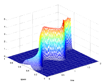
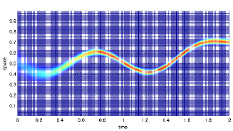
Figure 1: Test 1: Mass evolution $m_{i,k}^{\varepsilon}$

Test 2 (non-degenerate diffusion) We consider the same problem as in Test 1, but now we change the diffusion term choosing $\sigma=0.2$. Let us note that, in this case, the scheme reduce to the one proposed in [11]. The running cost and the initial distribution are chosen as in the previous tests. The density evolution is shown in Fig. 2, which has been computed with $\rho=6.35\cdot 10^{-3},h=\rho,\varepsilon=2\sqrt{h}$ and $\tau=10^{-3}$. The number of iterations for the fixed point method, to satisfy the stopping criteria with $\tau=10^{-3}$, is 6. Let us note that in this case the convergence is faster compared to the deterministic case in Test 1. A diffusive effect is observed during the whole time interval, which seems not very strong, since it is opposite to the one due to the running cost, which tends to concentrate the mass density around the sinusoidal curve.

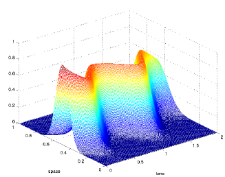
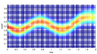
Figure 2: Test 2: Mass evolution $m_{i,k}^{\varepsilon}$

Test 3 (degenerate diffusion) We consider the same problem as in Test 1, but now we change the diffusion term choosing a scalar function

$$\sigma(t)=\max(0,0.2-|t-1|).$$

Note that $\sigma(t)=0$ for all $t\in[0,0.8]\cup[1.2,2]$. The running cost and the initial distribution are chosen as in the previous tests. The density evolution is shown in Fig. 3, which has been computed with $\rho=6.35\cdot 10^{-3},h=\rho,\varepsilon=2\sqrt{h}$ and $\tau=10^{-3}$. The number of iterations, for the fixed point method to satisfy the stopping criteria with $\tau=10^{-3}$, is 9. Let us note that in this case the rate of convergence, for the fixed point method, is between the rates for the two cases. We observe a diffusive effect during the time interval $[0.8,1.2]$, due to the non zero term $\sigma(t)$. When the diffusion stops to act, a time $t=1.2$ the density starts again to concentrate faster around the curve where $f$ is lower.

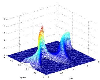
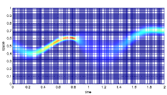
Figure 3: Test 1: Mass evolution $m_{i,k}^{\varepsilon}$

Table 1 shows the errors (6.2) computed varying all the parameters $(\rho,h,\varepsilon)$, according the balance $h=\rho$ and $\varepsilon=2\sqrt{h}$. In the first two columns of Table 1 we show the space and regularizing parameters, in the last two columns the errors for the value function and the density computed after 10 iterations of the fixed point algorithm.

Table 1: Parameters and errors

$\rho$	$\varepsilon$	$E(v^{\varepsilon,10})$	$E(m^{\varepsilon,10})$
$1.25\cdot 10^{-2}$	$0.2$	$1.72\cdot 10^{-6}$	$9.52\cdot 10^{-5}$
$6.25\cdot 10^{-3}$	$0.15$	$1.08\cdot 10^{-6}$	$1.17\cdot 10^{-4}$
$3.12\cdot 10^{-3}$	$0.1$	$1.82\cdot 10^{-6}$	$3.26\cdot 10^{-4}$

In Fig. 4, we show the behavior of the errors (6.2) in logarithmic scale on the $y$-axes versus the number of fixed-point iterations on the $x$-axes. We vary all the parameters according to the Table 1.

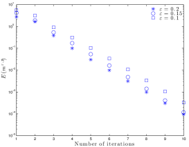
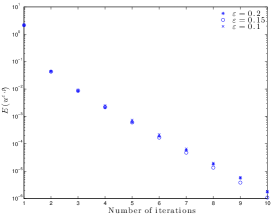
Figure 4: Errors: $E(m^{\varepsilon,p})$ (left) $E(u^{\varepsilon,p})$ (right) varying all the parameters $(\varepsilon,\rho,h)$ according to Table 1.

References

[1]
Y. Achdou, F. Camilli, and L. Corrias.
On numerical approximations of the Hamilton-Jacobi-transport
system arising in high frequency.
Discrete and Continuous Dynamical Systems- Series B,
19(2):629–650, 2014.
[2]
Y. Achdou, F. Camilli, and I. Capuzzo Dolcetta.
Mean field games: convergence of a finite difference method.
SIAM J. Numer. Anal., 51(5):2585–2612, 2013.
[3]
Y. Achdou and I. Capuzzo Dolcetta.
Mean field games: Numerical methods.
SIAM Journal of Numerical Analysis, 48-3:1136–1162,
2010.
[4]
L. Ambrosio, N. Gigli, and G. Savaré.
Gradient flows in metric spaces and in the space of probability
measures.Second edition. Lecture notes in Mathematics ETH
Zürich. Birkhäuser Verlag, Bassel, 2008.
[5]
G. Barles and P.E. Souganidis.
Convergence of approximation schemes for fully nonlinear second order
equations.
Asymptotic Anal., 4(3):271–283, 1991.
[6]
B. Bouchard and N. Touzi.
Weak dynamic programming principle for viscosity solutions.
SIAM Journal on Control and Optimization, 49(3):948–962, 2011.
[7]
L. Breiman.
Probability.
Addison-Wesley Publishing Company, Reading, MA, 1968.
[8]
F. Camilli and M. Falcone.
An approximation scheme for the optimal control of diffusion
processes.
RAIRO Modél. Math. Anal. Numér., 29(1):97–122, 1995.
[9]
F. Camilli and F. J. Silva.
A semi-discrete in time approximation for a first order-finite mean
field game problem.
Network and Heterogeneous Media, 7-2:263–277, 2012.
[10]
P. Cardaliaguet.
Notes on Mean Field Games: from P.-L. Lions’ lectures at
Collège de France.
Lecture Notes given at Tor Vergata, 2010.
[11]
E. Carlini and F. J. Silva.
Semi-lagrangian schemes for mean field game models.
In Decision and Control (CDC), 2013 IEEE 52nd Annual Conference
on, pages 3115–3120, Dec 2013.
[12]
E. Carlini and F. J. Silva.
A fully discrete semi-lagrangian scheme for a first order mean field
game problem.
SIAM Journal on Numerical Analysis, 52(1):45–67, 2014.
[13]
P. G. Ciarlet and J.-L. Lions, editors.
Handbook of numerical analysis. Vol. II.
Handbook of Numerical Analysis, II. North-Holland, Amsterdam, 1991.
Finite element methods. Part 1.
[14]
M.G. Crandall, H. Ishii, and P.-L. Lions.
User’s guide to viscosity solutions of second order partial
differential equations.
Bull. American Mathematical Society (New Series), 27:1–67,
1992.
[15]
F. Da Lio and O. Ley.
Uniqueness results for second-order bellman–isaacs equations under
quadratic growth assumptions and applications.
SIAM Journal on Control and Optimization, 45(1):74–106, 2006.
[16]
K. Debrabant and E. R. Jakobsen.
Semi-Lagrangian schemes for linear and fully non-linear diffusion
equations.
Math. Comp., 82(283):1433–1462, 2013.
[17]
A. Figalli.
Existence and uniqueness of martingale solutions for sdes with rough
or degenerate coefficients.
J. Funct. Anal., 253:109–153, 2008.
[18]
W.H. Fleming and H.M. Soner.
Controlled Markov processes and viscosity solutions.
Springer, New York, 1993.
[19]
D. Gomes and J. Saúde.
Mean Field Models, A Brief Survey.
Dynamic Games and Applications, pages 1–45, 2013.
[20]
O. Guéant.
Mean field games equations with quadratic hamiltonian: a specific
approach.
Mathematical Models and Methods in Applied Sciences, 22, 2012.
[21]
O. Guéant, J.-M. Lasry, and P.-L Lions.
Mean field games and applications.
In Paris-Princeton Lectures on Mathematical Finance
2010, volume 2003 of Lecture Notes in Math., pages 205–266. Springer,
Berlin, 2011.
[22]
M. Huang, P.E. Caines, and R.P. Malhamé.
Individual and mass behavior in large population stochastic wireless
power control problems: centralized and Nash equillibrium solutions.
Proc. 42nd IEEE-CDC, 2003.
[23]
M. Huang, P.E. Caines, and R.P. Malhamé.
Large populations stochastic dynamics games: closed-loop
McKean-Vlasov systems and the Nash certainly equivalence principle.
Comm. Inf. Syst., 6:221––251, 2006.
[24]
A. Lachapelle, J. Salomon, and G. Turinici.
Computation of mean field equilibria in economics.
Mathematical Models and Methods in Applied Sciences,
20-4:567––588, 2010.
[25]
J.-M. Lasry and P.-L. Lions.
Jeux à champ moyen I. Le cas stationnaire.
C. R. Math. Acad. Sci. Paris, 343:619–625, 2006.
[26]
J.-M. Lasry and P.-L. Lions.
Jeux à champ moyen II. Horizon fini et contrôle optimal.
C. R. Math. Acad. Sci. Paris, 343:679–684, 2006.
[27]
J.-M. Lasry and P.-L. Lions.
Mean field games.
Jpn. J. Math., 2:229–260, 2007.
[28]
A. Quarteroni, R. Sacco, and F. Saleri.
Numerical Mathematics (Second Ed.).
Springer, Berlin, 2007.
[29]
C. Villani.
Topics in Optimal Transportation.
Vol. 58 of Graduate Studies in Mathematics. American
Mathematical Society, Providence, RI, 2003.
[30]
J. Yong and X.Y. Zhou.
Stochastic controls, Hamiltonian systems and HJB equations.
Springer-Verlag, New York, Berlin, 2000.