Validation of Spherically Symmetric Inversion by Use of a Tomographic Reconstructed Three-Dimensional Electron Density of the Solar Corona

Abstract

Determination of the coronal electron density by the inversion of white-light polarized brightness ($pB$) measurements by coronagraphs is a classic problem in solar physics. An inversion technique based on the spherically symmetric geometry (Spherically Symmetric Inversion, SSI) was developed in the 1950s, and has been widely applied to interpret various observations. However, to date there is no study about uncertainty estimation of this method. In this study we present the detailed assessment of this method using a three-dimensional (3D) electron density in the corona from 1.5 to 4 $R_{\odot}$ as a model, which is reconstructed by tomography method from STEREO/COR1 observations during solar minimum in February 2008 (Carrington rotation, CR 2066). We first show in theory and observation that the spherically symmetric polynomial approximation (SSPA) method and the Van de Hulst inversion technique are equivalent. Then we assess the SSPA method using synthesized $pB$ images from the 3D density model, and find that the SSPA density values are close to the model inputs for the streamer core near the plane of the sky (POS) with differences generally less than a factor of two or so; the former has the lower peak but more spread in both longitudinal and latitudinal directions than the latter. We estimate that the SSPA method may resolve the coronal density structure near the POS with angular resolution in longitude of about 50^∘. Our results confirm the suggestion that the SSI method is applicable to the solar minimum streamer (belt) as stated in some previous studies. In addition, we demonstrate that the SSPA method can be used to reconstruct the 3D coronal density, roughly in agreement with that by tomography for a period of low solar activity (CR 2066). We suggest that the SSI method is complementary to the 3D tomographic technique in some cases, given that the development of the latter is still an ongoing research effort.

1 Introduction

The electron density is a fundamental parameter in plasma physics. Knowledge of the three-dimensional (3D) electron density structure is very important for our understanding of physical processes in the solar corona, such as the coronal heating and the acceleration of the solar wind (e.g., mun77; cra99). The density structure of the corona strongly affects the propagation of CMEs [Odstrčil and Pizzo (1999), Riley, Linker, and Mikić (2001), Odstrčil et al. (2002), Manchester et al. (2004)]. The density is also important for estimates of the Alfvén Mach number and compression rate of CME-driven shocks [Reames (1999), Sokolov et al. (2004), Manchester et al. (2005)], and for the interpretation of solar radio emission such as type II and type IV radio bursts produced by coronal eruptions [Caroubalos et al. (2004), Cho et al. (2007), Shen et al. (2013), Ramesh et al. (2013), Zucca et al. (2014)].

The K corona arises from Thomson scattering of photospheric white light from free electrons (e.g., bil66). Because the emission is optically thin, the measured signal is a contribution from electrons all along the line of sight (LOS). The derivation of the electron density in the K corona from the total brightness ($B$) or polarized radiance ($pB$) is a classical problem of coronal physics, first addressed by min30 and van50. Because of difficulties in generally separating the K-coronal component from the F-coronal component arising from interplanetary dust scattering (e.g., bil66; hay01), most of the inversion techniques are practical for $pB$ measurements. The F-coronal polarization is not very well understood (see reviews by kou85; kim98). It is generally accepted that the polarized contribution of the F corona can be ignored within 5 $R_{\odot}$ [Mann (1992), Koutchmy and Lamy (1985), Hayes, Vourlidas, and Howard (2001)], but some observations show that the F corona is almost unpolarized even at elongations ranging from 10 to 16 $R_{\odot}$ (bla66a, 1966b; bla67). In addition, the F corona dominates the total brightness of the corona beyond about 4 or 5 $R_{\odot}$ and make it difficult to recover the much fainter K-corona emission Saito, Poland, and Munro (1977); Koutchmy and Lamy (1985); Hayes, Vourlidas, and Howard (2001). To retrieve the electron density of the corona from a single 2D $pB$-image, one needs to assume some special geometries for the distribution of electrons along the LOS. The previous studies have modeled the electron density distribution in several ways, including the simple spherically symmetric model Van de Hulst (1950), the axisymmetric model Saito (1970); Munro and Jackson (1977); Quémerais and Lamy (2002), or the models that take into account large-scale structures, such as polar plumes in the coronal holes Barbey et al. (2008), or active streamers in the equatorial regions Guhathakurta, Holzer, and MacQueen (1996).

Figure 1.: Spherical cross section of the tomographic reconstructed 3D coronal electron density for CR 2066 at a heliocentric distance of 2.0 $R_{\odot}$. Two vertical solid lines marked with AE and AW indicate the positions of the east and west limbs in the COR1-A image observed at 12:00 UT on 8 February 2008, and those dashed lines with BE and BW the positions of east and west limbs in the COR1-B image at the same time. The symbols marked diamonds and pluses indicate the locations for the SSPA inversions shown in Figures fig:neva and fig:nevb. fig:necr

Among the above inversion methods, the spherically symmetric inversion (SSI) developed by van50 (called the Van de Hulst inversion thereafter), was the most representative and commonly used. He found that the density integral for $pB$ signals becomes invertible if the latitudinal and azimuthal gradients in electron density are weaker than the radial gradient (i.e., a local spherical symmetry approximation). This classic inversion technique has been applied to establish the standard density models of the coronal background at equator and pole in the solar minimum and maximum (see all00) and the density models of near-symmetric coronal structures such as streamers and coronal holes Saito, Poland, and Munro (1977); Gibson and Bagenal (1995); Guhathakurta and Fisher (1995); Guhathakurta, Holzer, and MacQueen (1996); Gibson et al. (1999). The SSI method was also used to analyze detailed density distribution of fine coronal structures observed in eclipses (e.g., kou94; nov96), and to derive the 2D density distribution of the entire corona Hayes, Vourlidas, and Howard (2001); Quémerais and Lamy (2002), when the spherical symmetry is assumed holding locally. The importance of the SSI method for coronal density determination has been demonstrated by wide applications of the derived densities such as in testing models of the acceleration mechanism of the fast solar wind Quémerais et al. (2007); Lallement et al. (2010), interpreting sources of type II and type IV radio bursts Cho et al. (2007); Shen et al. (2013); Ramesh et al. (2013); Zucca et al. (2014), and determining the coronal magnetic field strengths from fast magnetosonic waves by global coronal seismology Kwon et al. (2013).

However, in contrast to extensive applications, studies on evaluation of the SSI method are few in the literature. gib99 compared the white light densities to those determined from the density-sensitive EUV line ratios of Si ix 350/342 Å observed by SOHO/CDS, and found that densities determined from these two different analysis techniques match extremely well in the low corona for a very symmetric solar minimum streamer structure. Similarly, lee08 compared densities of various coronal structures determined by inverting MLSO MK4 $pB$ maps and from the line ratios of O vi 1032/1037.6 Å observed by SOHO/UVCS, and found that the mean densities in a streamer by the two methods are consistent, while the coronal densities for a coronal hole and an active region are within a factor of two. These results are encouraging, and suggest that the 2D white-light density distribution in coronal structures can be very useful for other studies, but a detailed assessment is required for its better application, such as information about the limitation of the SSI method and the uncertainty of derived densities. To achieve this goal, one may use synthetic $pB$ images from 3D densities of the corona reconstructed by tomographic techniques (fra02; fra07, 2010; vas08; kra09; but10; bar13), or simulated by global 3D MHD models Mikić et al. (1999); Linker et al. (1999); Usmanov et al. (2000); Groth et al. (2000); Hayashi (2005); Riley et al. (2006); Feng, Zhou, and Wu (2007); Hu et al. (2008); Lionello, Linker, and Mikić (2009); van der Holst et al. (2014).

Figure 2.: Cross sections of the tomographic 3D coronal density in the plane of the sky (POS), corresponding to positions of COR1-A (a) and COR1-B (b) at 12:00 UT on 8 February 2008. fig:nemap

The tomographic technique is a sophisticated method which reconstructs optically thin 3D coronal density structures using observations from multiple viewing directions. The use of this method in solar physics was previously proposed by dav94, and later this method has been applied to the SOHO/LASCO Frazin and Janzen (2002) and STEREO/COR1 data Kramar et al. (2009, 2014). For a solar coronal tomography based on observations made by a single spacecraft or only from the Earth-based coronagraph, data typically need to be gathered over a period of half solar rotation, so, generally, only structures that are stationary over about two weeks can be reliably reconstructed. Therefore, this technique is not applicable to eclipses or, perhaps, periods of high level of solar activity, although the 3D coronal electron density can be routinely computed Butala, Frazin, and Kamalabadi (2005); Kramar et al. (2009). Similarly, as global MHD models of the corona need measurements of photospheric magnetic field data over a solar rotation, it is also difficult using the MHD method to reconstruct dynamic or rapidly-evolving coronal structures matching to observations. Thus, the SSI analysis could be very useful in some cases when the tomography is not suitable. In addition, the SSI method is also useful in order to investigate the coronal density variability over a long term period (several solar cycles) when modern quality synoptic observations were not available and relate it to the modern state of the art reconstructions.

In this study, we choose the 3D coronal density obtained by tomography as a model in order to estimate uncertainties of the SSI method. vas08 compared the tomographic reconstruction and a 3D MHD model of the corona, and found that at lower heights the MHD models have better agreement with the tomographic densities in the region below 3.5 $R_{\odot}$, but become more problematic at larger heights. They also showed that the tomographic reconstruction has more smaller-scale structures within the streamer belt than the model can reproduce. Moreover, the tomographic reconstruction is entirely based on coronal observations, while the MHD models are primary based on photospheric boundary conditions. This suggests that the tomographic reconstructions are more realistic and thus may be more suitable to be used as a model in order to evaluate uncertainties of the SSI method.

This article is organized as follows. Section sctssi describes two SSI methods and their relationship. Section sctrlt presents the evaluation of the SSI method. We demonstrate the 3D density reconstruction by the SSI method based on real data in Section sctd3d. The discussion and conclusions as well as the potential extension of our work are given in Section sctdc.

Figure 3.: Synthetic $pB$ images based on the 3D coronal density model reconstructed by tomography. (a) Viewed from COR1-A, and (b) from COR1-B at 12:00 UT on 8 February 2008. Carrington longitudes of the viewing direction are marked at the bottom of the images. Solid lines mark the positions where the $pB$ intensity profiles shown in Figure fig:pblc are extracted. Short bars with a size of 0.31 $R_{\odot}$ show the scale, over which the $pB$ intensity is averaged across the radial cut. Four circles (dotted lines) at 1.6, 2.0, 2.5 and 3.0 $R_{\odot}$ mark the paths along which the density profiles are shown in Figure fig:neap.fig:pbmap

Figure 4.: Radial profiles of $pB$ for COR1-A (solid line) and COR1-B (dashed line), extracted along the radial cuts shown in Figure fig:pbmap. The error bars are the standard deviations for average over five pixels across the cut. fig:pblc

2 Spherically Symmetric Inversion Method

sctssi

Following derivations in bil66, $pB$ at a point, P, on the plane of sky (POS) can be expressed as,

$$pB(\rho)=\frac{B_{\odot}}{1-u/3}\left(\frac{3\sigma_{T}}{16}\right)\int_{LOS}[(1-u)A(r)+uB(r)]\frac{\rho^{2}}{r^{2}}N(s)ds,\ilabel{eqpb}$$ (1)

where the POS is defined as a plane crossing the Sun’s center and perpendicular to the LOS, $N$ is the electron density, $\rho$ is the perpendicular distance between the LOS and Sun center, $r$ is the radial distance from the Sun center, and $s$ is the distance measured from P along the LOS. These distances are related by $r^{2}=\rho^{2}+s^{2}$. $B_{\odot}$ is the mean solar brightness. $\sigma_{T}=\frac{8}{3}\pi{r}_{0}^{2}=6.65\times 10^{-25}$ cm², is the Thompson scattering cross section for a single electron, where ${r}_{0}$ is the classical electron radius. Note that $r_{0}^{2}=7.94\times 10^{-26}$ cm² is the “Thompson scattering cross section” as referred to in Billings Billings (1966). $u$ is the limb darkening coefficient. In addition, $A(r)$ and $B(r)$ are geometrical factors given by Billings Billings (1966)

$$A(r) = {\rm cos}\Omega\,{\rm sin}^{2}\Omega,$$ (2)

$$B(r) = -\frac{1}{8}\left[1-3\,{\rm sin}^{2}\Omega-{\rm cos}^{2}\Omega\left(\frac{1+3\,{\rm sin}^{2}\Omega}{{\rm sin}\Omega}\right){\rm ln}\left(\frac{1+{\rm sin}\Omega}{{\rm cos}\Omega}\right)\right],$$ (3)

where the angle $\Omega$ is defined by ${\rm sin}\Omega=R_{\odot}/r$.

If electron density is a function of $r$ only, Equation (eqpb) can be written in the form

$$pB(\rho)=C\int_{\rho}^{+\infty}[(1-u)A(r)+uB(r)]N(r)\frac{\rho^{2}dr}{r\sqrt{r^{2}-\rho^{2}}},\ilabel{eqpbr}$$ (4)

where $r$ and $\rho$ are in units of $R_{\odot}$, and $C=(3/8)\sigma_{T}R_{\odot}B_{\odot}/(1-u/3)$. van50 developed a technique for the inversion of $pB$ measurements (called the Van de Hulst inversion). To implement this technique, one needs first to fit the $pB$ data using a curve in the polynomial form, specifically,

$$pB(\rho)=\sum_{k}a_{k}\rho^{-k}.\ilabel{eqpbsum}$$ (5)

Once the coefficients $a_{k}$ are determined, the solution of Equation (eqpbr) is then given by

$$N(r)=\frac{\sum_{k}(a_{k}/c_{k+1})r^{-(k+1)}}{C((1-u)A(r)+uB(r))},\ilabel{eqnr}$$ (6)

where

$$c_{k}=\int_{0}^{\pi/2}{\rm cos}^{k}{\phi}\,d\phi=\frac{\sqrt{\pi}}{2}\frac{\Gamma((k+1)/2)}{\Gamma(k/2+1)},$$ (7)

where $\Gamma$ is the gamma function. Note that the constant $C$ here is different from that in van50, because we have used the expression of $pB$ in bil66. More generally, the index $k$ of radial power law in Equation (eqpbsum) is real but not necessarily integer valued. This leads to the modified Van de Hulst technique assuming $pB(\rho)=\sum_{k}{a_{k}}\rho^{-d_{k}}$, where $a_{k}$ and $d_{k}$ are the fit coefficients, then $c_{k+1}$ and $r^{-(k+1)}$ in Equation (eqnr) need to be replaced with $c_{d_{k}+1}$ and $r^{-(d_{k}+1)}$ (e.g., sai77; guh96; gib99).

hay01 developed another SSI technique by assuming the radial electron density distribution in the polynomial form, $N(r)=\sum_{k}b_{k}r^{-k}$, and have used it to the inversion of total brightness observations. We here adopt this technique for the $pB$ inversion, and call it the spherically symmetric polynomial approximation (SSPA) method for short. By substituting the polynominal for $N(r)$ in Equation (eqpbr), we obtain

$$pB(\rho)=\sum_{k}b_{k}G_{k}(\rho),\ilabel{eqpbg}$$ (8)

where

$$G_{k}(\rho)=C\int_{\rho}^{+\infty}[(1-u)A(r)+uB(r)](r^{-k})\frac{\rho^{2}dr}{r\sqrt{r^{2}-\rho^{2}}},\ilabel{eqgkr}$$ (9)

For easier calculation, using the substitution $r=\rho/{\rm cos}\theta$ the integral can be transformed into

$$G_{k}(\rho)=C\rho^{-k+1}\int_{0}^{\pi/2}[(1-u)A(r(\theta))+uB(r(\theta))]{\rm cos}^{k}\theta\,d\theta,\ilabel{eqgktht}$$ (10)

where $\theta$ is the angle from the POS to a direction from the Sun center to a point of distance $s$ along the LOS. Since the integral $G_{k}(\rho)$ can be numerically calculated for all desired impact distances $\rho$ and exponents $k$, substituting the observed $pB$ curve along a radial trace for the left-hand side of Equation (eqpbg) the only unknowns are the coefficients $b_{k}$. We determine the coefficients by a multivariate least-squares fit to the curve of $pB(\rho)$ (using the function of svdfit provided by IDL, Interactive Data Language). The radial distribution of electron density is then obtained by substituting the resulting coefficients directly into the polynomial form. To select appropriate degrees of polynominal we did some experiments using coronal density models for the region between 1.5 and 6 $R_{\odot}$ in sai77, and found that choosing the first five terms ($k=1-5$) can determine $N(r)$ with the relative errors within 5% and reproduce $pB$ measurements with the relative errors within 1%. We thus use the 5-degree polynomial fits for all the SSPA inversions in our study.

To look into the relationship between the SSPA and Van de Hulst inversions theoretically, we use Taylor series to approximate the functions $A(r)$ and $B(r)$ in the case when $r>1$ with $r$ in unit of $R_{\odot}$,

$$A(r) \approx \left(\frac{1}{r}\right)^{2}-\frac{1}{2}\left(\frac{1}{r}\right)^{4}-\frac{1}{8}\left(\frac{1}{r}\right)^{6}+...\,,$$ (11)

$$B(r) \approx \frac{2}{3}\left(\frac{1}{r}\right)^{2}-\frac{4}{15}\left(\frac{1}{r}\right)^{4}-\frac{3}{40}\left(\frac{1}{r}\right)^{6}+...\,.$$ (12)

For the Taylor polynomial approximations of degree six above, the relative errors are less than 1% when $r>1.5$. Since $A(r)$ and $B(r)$ are on the order of $O(1/r^{2})$ for very large $r$, by keeping only the terms of $1/r^{2}$ we have $(1-u)A(r)+uB(r)\approx(1-u/3)(1/r^{2})$, which corresponds to the point source approximation Frazin et al. (2010). Applying this approximation to Equation (eqnr) for the Van de Hulst inversion, we obtain

$$N(r)=\frac{1}{C(1-u/3)}\sum_{k}\left(\frac{a_{k}}{c_{k+1}}\right)r^{-(k-1)}.\ilabel{eqnrapx}$$ (14)

This verifies the polynomial form of $N(r)$ assumed in the SSPA method. Conversely, if $N(r)$ is given in the same form as Equation (eqnrapx), likewise we can recover $pB(\rho)=\sum_{k}a_{k}\rho^{-k}$ as assumed in the Van de Hulst inversion from the SSPA inversion using Equations (eqpbg) and (eqgktht) with the point source approximation for $(1-u)A(r)+uB(r)$. Thus, we have proved that the SSPA and Van de Hulst inversions are identical on the order of $O(1/r^{2})$, and their difference in higher orders can be reduced by increasing the degrees of $k$. Note that the above analysis is also valid for the case when $k$ is real. In Section sctstrm, we will show that the coronal densities determined from COR1 images by the SSPA and Van de Hulst inversions with $k$=5 are almost identical. Therefore, the assessment of the SSPA inversion in the following is equivalent to that of the Van de Hulst inversion.

Figure 5.: (a) and (b): The synthetic $pB$ data (denoted with pluses) along a radial cut shown in COR1-A and -B images in Figure fig:pbmap, and their least-squares fit (solid line) using the SSPA method. (c) and (d): The density profiles derived with the SSPA inversion (thin solid line) and the Van de Hulst inversion (dashed line), as well as the model densities in the POS (thick solid line). Note that in panel (d) the density profiles obtained by the SSPA and the Van de Hulst inversions are overlaid completely. For comparison, the $pB$ profile and the density model for the equatorial background derived by Saito, Poland, and Munro (1977) from the Skylab data are plotted with dot-dashed lines. In (c) and (d) the overplotted curves also include the solar minimum streamer densities (dotted line) obtained by Gibson et al. (1999) from Mauna Loa/LASCO C2 data. fig:pbinv

3 Evaluation of the SSI Method

sctrlt

3.1 Coronal Density Model for Evaluation of SSI Method

scttt As a model for evaluation of SSI method we used a 3D coronal electron density obtained by tomography method applied to white-light coronagraph data Kramar et al. (2009). The data were acquired by the inner coronagraph (COR1) telescopes aboard the twin Solar Terrestrial Relation Observatory (STEREO) spacecraft. COR1 observes the white-light K corona from about 1.4 to 4 $R_{\odot}$ in a waveband of 22.5 nm wide centered on H$\alpha$ line at 656 nm with a time cadence of 5 minutes. Regularized tomographic inversion method by kra09 with the limb darkening coefficient $u$=0.6 provided the reconstruction of a 3D coronal electron density for the period of 2008 February 1–14 (consisting of 28 $pB$ images from COR1-B) that corresponds to Carrington Rotation (CR) 2066. The scattered light in the $pB$ data was removed by subtracting a combination of the monthly minimum and the roll minimum backgrounds Thompson et al. (2010). The reconstruction domain is a $128^{3}$ rectangular grid covering a spherical region between 1.5 and 4 $R_{\odot}$. We evaluate the SSPA inversion method using this 3D density reconstruction as a model.

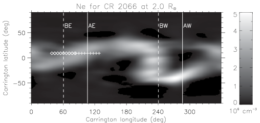
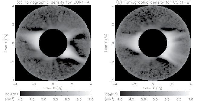
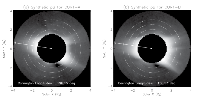
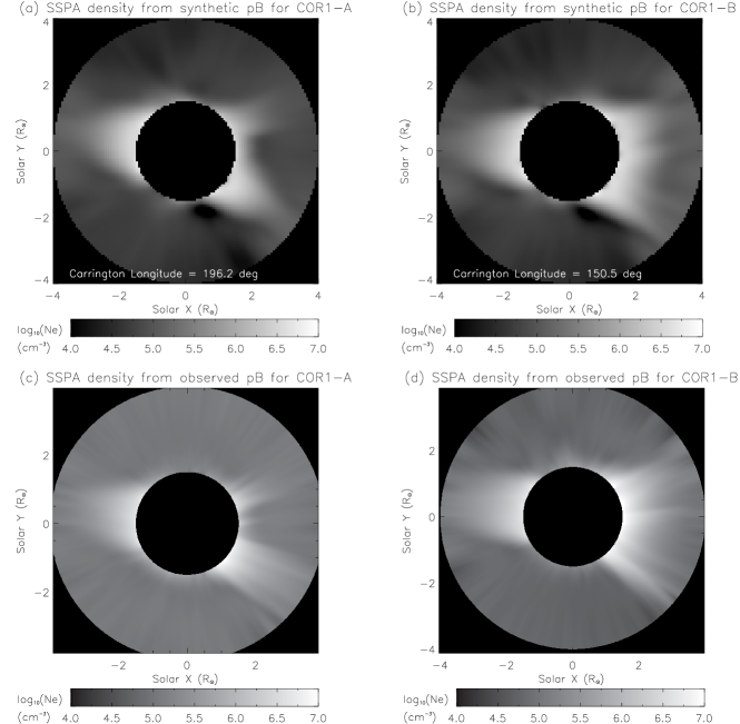
In order to synthesize $pB$ images observed by COR1-A and -B at a given time, we first determine the orbital positions of the spacecraft in Carrington coordinates using the routine $get\_stereo\_lonlat$ provided by SolarSoftWare (SSW). The 3D density grid is then transformed from the Carrington heliographic system to the projected coordinate system viewed from STEREO-A or -B Thompson (2006). Therefore, the LOS integral of $N(r)$ in Equation (eqpb) becomes a simple summation in the $z$-direction (defined along LOS). Figure fig:necr shows the tomographic reconstructed 3D coronal electron density at 2 $R_{\odot}$. Figure fig:nemap shows the density distributions of the corona in the POS for COR1-A and -B at 12:00 UT on 8 February 2008. Figure fig:pbmap shows the corresponding synthetic $pB$ images, which represent the ideal measurements without contamination by the scattered light and instrumental noises.

Figure 6.: Comparison of the SSPA density profile (dashed line) with the model densities in 13 angular sections (solid lines). The thick black line stands for the case in the POS, while thin color lines for cases with angles relative to the POS to be $\pm$5, 10, 15, 20, 25, 30 degrees, where the negative value represents an angle measured inward and the positive value an angle measured outward. (a) For COR1-A. (b) for COR1-B. $L_{\rm AE}$ and $L_{\rm BE}$ marked in (a) and (b) represent the longitude of the east limb in COR1-A and -B, respectively. fig:pbinm

3.2 Radial Distribution of Electron Densities in Solar Minimum Streamer

sctstrm Coronal streamers are the most conspicuous, large-scale structures in the extended corona. The streamer belt is a usually continuous sheet of enhanced density associated with the magnetic neutral sheet or the current sheet (sch73; guh96; sae07; kra09, 2011). Its shape gets progressively deformed from a rather flat plane at minimum solar activity to a highly warped surface at maximum solar activity (e.g., hu08). Some previous studies have suggested that the SSI assumptions are suitable to symmetric streamers at low latitude, in particular, the solar minimum streamer belt (e.g., guh95; gib95; gib99). Here we first test the SSPA inversion of the solar minimum streamer belt. A streamer belt during CR 2066 corresponding to solar minimum of Solar Cycles 23$/$24 is shown in Figure fig:necr.

Figure 7.: The electron density profiles derived by the SSPA inversion (dashed line) as a function of longitudes. The analyzed radial trace is located at the position with Carrington latitude of 9^∘ and longitude marked at the top of each panel and shown with pluses in Figure fig:necr. The solid line in each panel represents the corresponding model densities in the POS. fig:neva

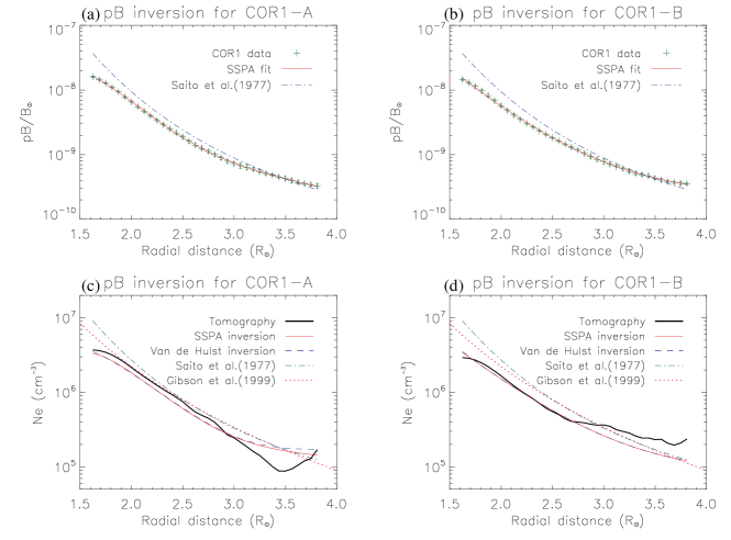
For instance, we use the synthetic $pB$ images at 12:00 UT on 8 February 2008 when the separation angle between STEREO-A and -B was about 45^∘. Figure fig:pbmap shows that the streamer belt on the east limb is almost edge-on, as inferred from the similar appearance in COR1-A and -B. In the edge-on condition, the coronagraph is looking along the streamer belt; i.e., where all the streamers are at the same latitude behind each other along the LOS. In contrast, the streamer belt on west limb in COR1-B is face-on, showing a distinctly different shape from that in COR1-A. We choose a radial trace near the middle of the east-limb streamer (see marked positions in Figure fig:pbmap), where the $pB$ profiles for COR1-A and -B are nearly identical (Figure fig:pblc), and suppose that this location best meets the SSI condition. We then derive the radial distribution of electron density by fitting the $pB$ data along this radial trace between 1.6 and 3.9 $R_{\odot}$ using both the SSPA method and the Van de Hulst technique ($pb\_inverter$ with $k$=5 in SSW) for an illustrated comparison, and show the inversion results in Figure fig:pbinv. Note that since COR1 does not perform well at $\rho\lesssim$1.55 $R_{\odot}$ at some position angles due to interference from the occulter (see fra12), this led to defective $pB$ signals and thus unreliable reconstructions within this region, so we constrain all SSPA inversions in the following to regions with $\rho\geq 1.6R_{\odot}$.

Figure 8.: Same as Figure fig:neva but in the case for COR1-B. Locations of the analyzed radial trace are marked with diamonds in Figure fig:necr, whose latitude is 9^∘ and longitude is marked at the top of each panel. The solid line represents the model densities in the POS while the dashed line represents the SSPA densities.fig:nevb

We find that the electron densities obtained from both $pB$ inversion methods agree well in radial distribution with the model 3D densities in the POS for selected longitudes corresponding to the edge-on streamer positions (see Figure fig:pbinv (c) and (d)). This confirms our theoretical prediction that the PPSA and the Van de Hulst inversions are equivalent. The average ratio of the SSPA to the model densities along the selected radial cut between 1.6 and 3.0 $R_{\odot}$ is 0.86$\pm$0.06 and 0.95$\pm$0.10 for COR1-A and -B, respectively. Note that weak increase in density with height between 3.5 and 4.0 $R_{\odot}$ may be due to FOV effects (see discussion in Section sctdc). In addition, the lower panels of Figure fig:pbinv show that both the tomographic and SSPA density profiles determined for streamers are comparable (with differences by $\sim$20%) to the previous obtained by SSI method in the solar minimum Gibson et al. (1999); Saito, Poland, and Munro (1977).

To examine to what extent the SSPA solution is consistent with the 3D density model, we compare the SSPA density profile with the model density profiles in 13 angular sections to the POS within 30^∘ in Figures fig:pbinm(a) and (b), which show that the SSPA solution is closest to the distribution of 3D densities in the POS. This is as expected because the $pB$ integrals along the LOS are most heavily weighted toward the regions near the POS (see que02; fra10).

Figure 9.: The coronal densities at 1.6, 2.0, 2.5, 3.0, and 3.5 $R_{\odot}$ as a function of Carrington longitudes, derived with the SSPA inversion (dashed lines) in comparison with those by the model in the POS (solid lines). The Carrington latitude of the analyzed radial trace is 9^∘. (a) For COR1-A. (b) For COR1-B. The vertical dotted lines indicate the middle position of the analyzed longitude range.fig:netim

Figure 10.: The 2D coronal density derived using the SSPA method from the synthetic $pB$ images, corresponding to positions of COR1-A (a) and COR1-B (b) at 12:00 UT on 8 February 2008. Carrington longitudes of the viewing direction are marked at the bottom of the density maps. (c) and (d): Same as (a) and (b) but derived from the real observed $pB$ images at the same time. fig:ne2d

3.3 Longitudinal and Latitudinal Dependence of the Streamer Density

sctsdd We evaluate the SSPA inversion of the streamer as a function of longitude in the following. This corresponds to make the SSPA inversion of synthetic $pB$ images at different “virtual observing times”. We synthesize the $pB$ images at nine times for COR1-A and -B, in a period from 20:00 UT, 6 February to 04:00 UT, 10 February with intervals of 10 hours, centered at 12:00 UT on 8 February 2008 (the time for the instance analyzed in the last section). The Sun rotated by 44^∘ over this period, approximately equal to the separation angle between STEREO-A and B. So the ending-time location analyzed in COR1-A is approximately superposed with the starting-time location in COR1-B as shown in Figure fig:necr. We fit the $pB$ data along the same radial trace between 1.6 and 3.9 $R_{\odot}$ at these nine times using the SSPA method. Figures fig:neva and fig:nevb show comparisons of the obtained density profiles with the model densities in the POS for COR1-A and COR1-B, respectively. For the analyzed locations with longitude between $60^{\circ}$ and $106^{\circ}$ (approximately between the limbs $BE$ and $AE$ as shown in Figure fig:necr), we find that the density profiles derived by SSPA method have the similar shape as the model profiles over almost the whole FOV range (1.6–3.8 $R_{\odot}$), but the magnitudes are smaller than the model by about 20%–50%. The reason for good agreements during this period could be that the streamers in the LOS at the analyzed location are near the POS. The model density increases near the edge of FOV seen in Figures fig:neva(c)-(e) and Figures fig:nevb(g)-(i) likely result from the FOV effects in the tomographic inversion Frazin et al. (2010). Figure fig:netim shows the SSPA density as a function of longitude at five heights (1.6, 2.0, 2.5, 3.0 and 3.5 $R_{\odot}$). The comparison with the model confirms the result above that the better agreement lies at the locations with the longitude in 60^∘–106^∘. We also find that the agreement tends to be better at lower heights. The average difference between the SSPA and model densities are $\sim$20% for the region between 1.6 and 2.0 $R_{\odot}$, while $\sim$40%–50% for 2.5–3.5 $R_{\odot}$. The reason could be that the SSI condition is better meet at lower heights where the streamer has a larger extent in the LOS, and thus the LOS integration in Equation (eqgktht) over a very long distance (compared to the width of the streamer) becomes more reasonable.

Now we evaluate the latitudinal dependence of SSPA inversions of the corona. By assuming that the SSI condition holds locally for all angular positions around the Sun, the 2D coronal density can be derived from a $pB$ image by fitting the radial profile at each angular position using the SSPA method. For the case analyzed in Section sctstrm, we reconstruct 2D coronal densities in the POS by fitting radial profiles between 1.6 and 3.7 $R_{\odot}$ for 360 position angles with intervals of 1^∘ from both synthetic and observed $pB$ images, and show the results in Figure fig:ne2d. Compared to the tomographic densities in the POS (see Figure fig:nemap), the SSPA coronal densities determined from the observed images do not show very low-density regions around streamers, while those from the synthetic images have a small region of zero (or negative) densities at the southern side of the west-limb streamer, where the synthetic $pB$ signals are very low (below the background level in non-streamer regions). The zero density regions in tomographic reconstructions could be caused either (or both) due to coronal dynamics or due to real very small density in these coronal regions (see discussions in Section sctdc).

For a quantitative comparison, we plot the SSPA and model density profiles as a function of position angles at four heights (1.6, 2.0, 2.5, and 3.0 $R_{\odot}$) in Figure fig:neap. For the three edge-on streamers marked with S1–S3, we measure their peak densities and angular widths (in FWHM). The ratio of peak densities from the SSPA to the model is on average 0.82$\pm$0.06, 0.72$\pm$0.09, and 0.62$\pm$0.12, and the ratio of angular widths is on average 1.24$\pm$0.02, 1.67$\pm$0.12, and 1.90$\pm$0.27 at 2.0, 2.5, and 3.0 $R_{\odot}$, respectively. The results indicate that the SSPA inversion underestimates the peak density of streamers by about 20%–40%, while overestimates the angular width by about 20%–90%. The increase of deviations with height in the peak density of streamers by the SSPA method from the model may be caused by narrowing of the streamer (belt) with height (see Figure 2 of kra09). As the streamer width along the LOS decreases with the height, the condition for the SSI assumption becomes worse. The reason for the latitudinal spreading of the SSPA density relative to the model may lie in that the analyzed streamers are not exactly edge-on, i.e., the streamer belt at the analyzed locations is actually tilted somewhat away from the equatorial direction (or the LOS near the limb, see Figure fig:necr). In such a case at the locations near the edge of streamer in the $pB$ image the contribution is larger from points along the LOS behind or in front of the POS, leading to an overestimation of the model density in the POS by the SSPA inversion at these places. In addition, we notice for the face-on streamer (marked S4) in COR1-B, its SSPA density profiles are consistent with the model densities as well, this is because this streamer is by coincidence located near the POS at this instance (Figure fig:necr).

In Figure fig:neap, we also compare the SSPA densities inverted from the synthetic $pB$ image with those from the observed $pB$ image, and find that they are generally consistent except in the region near the occulter of COR1, where the SSPA inversions from the observed $pB$ are much larger ($\sim$2–3 times) than the model densities (see panels (a) and (e) in Figure fig:neap). The version of tomographic reconstruction used here most likely underestimated the density there as the solution at grid points close to the occulter is less constrained by the observational data.

Figure 11.: The coronal densities along four circular paths at 1.6 (a), 2.0 (b), 2.5 (c), and 3.0 $R_{\odot}$ (d) for COR1-A. The position angle is counted anticlockwise relative to the north pole. For each circle its eastern part (position angles 0^∘–180^∘) has the longitude of 106.2^∘, and its western part has the longitude of 286.2^∘. The solid line represents the model densities, and the dashed line and the dotted line represent the SSPA densities from the synthetic and observed $pB$ images, respectively. (e)-(h): Same as panels (a)-(d) but for COR1-B. For each circle its eastern part has the longitude of 60.5^∘, and its western part has the longitude of 240.5^∘.fig:neap

Figure 12.: The SSPA-reconstructed 3D coronal densities from the two-week dataset of COR1 $pB$ images. (a)-(c): The spherical cross sections at 1.6, 2.0, and 2.5 $R_{\odot}$ for COR1-A, and (d)-(f) for COR1-B. In panels (a), (b), (d) and (e), the dotted line and the dashed line represent the positions of the east limb and the west limb, respectively, of the earliest-observed $pB$ image (at 00:25 UT, 1 February 2008). In panels (c) and (f), the vertical dotted and dashed lines represent the positions of the east limb and west limb, respectively, for all $pB$ images used in the reconstructions. fig:synab

Figure 13.: The ratio of tomographic density to the SSPA average density for COR1-A and -B at 1.6, 2.0, and 2.5 $R_{\odot}$ for two cases. (a)-(c): The case for the SSPA 3D coronal density obtained using synthetic $pB$ data based on the 3D density model. (d)-(f): The case for the SSPA 3D coronal density obtained using the real $pB$ data observed by COR1-A and -B. The colors represent the ratio values in a range 0–5 (see color bars at the bottom). A version with continuous color scale is available as Electronic Supplementary material.fig:syncp

4 Reconstruction of the 3D Coronal Density using SSPA Method for CR 2066

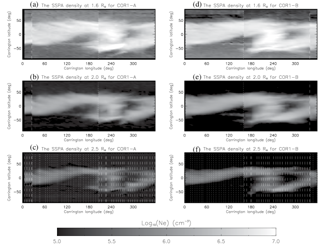
sctd3d In the above sections, we evaluated the SSPA method by comparing the derived density distribution as a function of radial distance, longitude and latitude with the 3D tomographic model. The assessments indicate that the SSPA inversion can determine the 2D coronal density from a $pB$ image, which approximately agrees with the 3D tomographic densities for streamers near the POS. This suggests that we may reconstruct a 3D density of the corona by applying the SSPA inversion to a 14 day data set from COR1-A or -B. In this section, we demonstrate the SSPA 3D density reconstructions using the same data set (consisting of 28 $pB$ images from COR1-B) as used for the reconstruction of 3D tomographic model, and the simultaneous COR1-A data set. The data cadence of about 2 images per day corresponds to a longitudinal step of about $6^{\circ}$. First we determine the 2D density distribution by fitting the radial $pB$ data between 1.6 and 3.7 $R_{\odot}$ using the SSPA inversion at 142 angular positions (with intervals of 2.5^∘) surrounding the Sun for each image. Then we map the east-limb and west-limb density profiles of all images to make a synoptic map at a certain height, based on their Carrington coordinates (neglecting the inclination of the solar rotational axis to the ecliptic). A 3D density reconstruction is made of 25 synoptic maps for the radial heights from 1.5 to 3.9 $R_{\odot}$ with an interval of 0.1 $R_{\odot}$. For each synoptic map, we convert the irregular grid into the regular grid using the IDL function, trigrid. Although the 3D density reconstruction can be made using the SSPA method from the COR1 data with a cadence as high as 5 minutes, the higher temporal resolution may not help improve its actual angular resolution in longitude due to intrinsic limitations of the SSPA method (see Appendix).

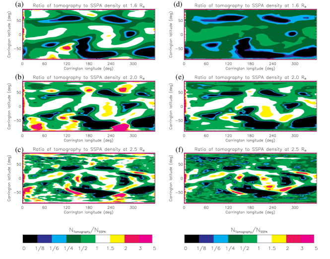
Figure fig:synab shows the SSPA-reconstructed 3D coronal density at 1.6, 2.0 and 2.5 $R_{\odot}$ for COR1-A and -B. Some discontinuities of the density are seen at two longitudes which separate the two regions made of the east-limb and west-limb inversions. These flawed structures may be due to temportal changes of streamers and/or the effect due to neglecting the solar axial tilt in the reconstruction. We smooth these discontinuities by averaging the two reconstructions from COR1-A and COR1-B and then make a $10^{\circ}\times 10^{\circ}$ smoothing. In Figure fig:syncp, we show the ratio of tomographic density to the SSPA average density for the COR1-A and -B reconstructions with smoothing for two cases, one for the SSPA densities obtained using the synthetic data (panels (a)-(c)), and the other for the SSPA densities obtained using the real data (panels (d)-(f)). Both cases indicate that the density ratios in the streamer belt are very close to 1, within a factor of two or so ($\sim$0.5–1 at 1.6 $R_{\odot}$, $\sim$1–2 at 2.0 $R_{\odot}$, and $\sim$1–3 at 2.5 $R_{\odot}$). The good consistency validates that the SSI assumptions are very appropriate for the streamer belt in the solar minimum.

For a quantitative comparison between the tomography and the SSPA densities (obtained from real data), we also show their density profiles along an equatorial cut in Figure fig:synpf. We find that they best match at 2 $R_{\odot}$. The same result is also indicated by the pixel-to-pixel scatter plots in Figure fig:pxsct. We obtain the ratio of the SSPA to the tomographic average density is 1.02, and their linear Pearson correlation coefficient is 0.93 for the reconstructions at 2 $R_{\odot}$. In addition, the scatter plots show that the dispersion is larger for those pixels with smaller values, where the SSPA densities are much larger than those obtained by the tomography.

Figure 14.: Comparison of the SSPA density profiles with the tomographic density profiles (thick solid line) along the equator at (a) 1.6, (b) 2.0, and (c) 2.5 $R_{\odot}$. The dotted and the dashed lines represent the SSPA coronal densities for COR1-A and -B, respectively, while the thin solid line represents their average with a 10-degree smoothing.fig:synpf

Figure 15.: The pixel-to-pixel scatter plots of the SSPA 3D coronal density (averaged for COR1-A and -B with a 10-degree smoothing) versus the tomographic 3D coronal density, at (a) 1.6, (b) 2.0, and (c) 2.5 $R_{\odot}$. The linear Pearson correlation coefficient ($\rho_{X,Y}$) and the ratio of the average densities ($<Y>/<X>$) are marked in each plot. fig:pxsct

5 Discussion and Conclusions

sctdc In this study, we have, for the first time, evaluated the SSI method using the 3D model of the coronal electron densities reconstructed by tomography from the STEREO/COR1 $pB$ data. Our study is instructive for more efficient use of the SSI technique to invert the $pB$ observations from ground- and space-based coronagraphs, in particular, the COR1 data. We demonstrate both theoretically and observationally that the SSPA method and the Van de Hulst inversion are equivalent SSI techniques when the radial densities or $pB$ signals are assumed in the polynomial form of high degrees (more than two). The polynomial degree of five is suitable for COR1 data inversions. Thus, assessment results of the SSPA method can also be applied to the Van de Hulst inversion technique. We determine radial profiles of the streamer density from the COR1-A and -B synthetic $pB$ images as well as their longitudinal and latitudinal dependencies. We find that the SSPA density values are close to the model for the core of streamers near the POS, with differences (or uncertainties if we regard the model input as a true solution) typically within a factor of $\sim$2. This result is consistent with those evaluated using UV spectroscopy Gibson et al. (1999); Lee et al. (2008). We find that the SSPA density profiles tend to better match the model at lower heights ($\lesssim$ 2.5 $R_{\odot}$). Our results confirm the suggestion in some previous studies that the SSI assumption is appropriate for the edge-on streamers or the streamer belt during the solar minimum. We suggest that the edge-on condition for streamers may be determined by tomography method or by examining the consistency between simultaneous $pB$ measurements from COR1-A and -B in radial distribution, when the two spacecraft have a small angular separation (e.g., less than 45^∘). We also find the SSPA streamer densities are more spread in both longitudinal and latitudinal directions than in the model.

We demonstrate the application of the SSPA inversion for reconstructions of the 3D coronal density near the solar minimum, and show that the SSPA 3D density for the streamer belt is roughly consistent in both position and magnitude with the tomographic reconstruction. The synoptic density maps derived by the SSPA method show some discontinuities at the longitudes that separate the regions made of the east- and west-limb inversions. These discontinuities may be due to temporal changes of coronal structures and/or the effect of tilt of the solar rotation axis on the poles’ visibility that is not considered. They can be smoothed out during post-processing by smoothing and averaging the density distributions from COR1-A and -B, but such treatments will reduce the spatial resolution. In comparison, the tomographic inversion can fully take into account the tilt effect of the solar pole and produce the density distributions smoother in these discontinuity regions Frazin and Janzen (2002); Kramar et al. (2009). We estimate that the SSPA method may resolve the coronal density structure near the POS with an angular resolution of $\sim$50^∘ in longitudinal direction. Given this limitation, the SSPA reconstruction using $pB$ data with higher cadence (e.g., more than three images per day) would not help improve its actual angular resolution.

Although the current state of the tomographic method has allowed to routinely obtain the 3D coronal densities, we speculate that the SSI method could be complementary to the tomography when used for the interpretation of observations in such cases as during maximum of solar activity, in some regions where tomography gives zero density values, or in the regions near the edges of FOV.

The zero density values in the tomographic reconstruction (so called “zero-density artifacts”, ZDAs) could be caused either (or both) due to coronal dynamics Frazin and Janzen (2002); Frazin et al. (2007); Vásquez et al. (2008); Butala et al. (2010), or due to real very small density in these coronal regions which are below the error limit in the tomography method Kramar et al. (2009). The latter reason is also supported by results of MHD modeling Airapetian et al. (2011). In the former case, the SSI method could be complementary to tomography, while in the latter case the SSPA method gives much larger values than in the tomographic model. The FOV artifacts in the tomography are due to the finite coronagraph FOV that causes the reconstructed density to increase at the regions close to the outer reconstruction domain Frazin et al. (2010); Kramar et al. (2009). However, this FOV artifacts can be reduced by extending the outer reconstruction domain beyond the coronagraph FOV limit Frazin et al. (2010); Kramar et al. (2013). Another way to obtain more correct density values in this region could be by using the SSPA method which does not imply strict outer boundaries for LOS integration. Thus the estimate of uncertainties of the SSPA method should be limited to the regions with distances less than about 3.5 $R_{\odot}$ for the tomographic model used. Also, the use of MHD model in order to produce artificial data can be useful for this test. However this will be a subject of future research.

The tomography generally assumes that the structure of the corona is stable over the observational interval, e.g., two weeks of observations made by a single spacecraft, although for some coronal regions that are exposed to the spacecraft for only about a week during the observation the stationary assumption can be reduced to about a week Kramar et al. (2011). However, such an assumption is hard to meet during solar maximum or times of enhanced coronal activity. The CME catalog in the NASA CDAW data center shows that the CME occurrence rate increases from $\sim$0.5 per day near solar minimum to $\sim$6 near solar maximum during Solar Cycle 23 Gopalswamy et al. (2003); Yashiro et al. (2004). Although our assessment results for the SSPA method are based on a static coronal model, their validity may not be limited to the static assumption. Because the key factor for the SSPA inversion for obtaining a good estimate of the 2D coronal density is an instantaneous (local) symmetric condition for coronal densities along the LOS. The minimal size of this local symmetry is limited by the angular resolution in longitude which is about $50^{\circ}$. Therefore, the SSI method can be used to estimate the density of a dynamic coronal structure in terms of weighted average over the region with this angular size in longitude. For this reason it may be a better choice to use a combination of the tomography and the SSI inversions for interpretations of radio bursts and shocks produced by CMEs in the case when coronal structures of interest evolve quickly with time Lee et al. (2008); Shen et al. (2013); Ramesh et al. (2013). In addition, the SSI method is also often applied to the cases when observational data are not suitable for tomography, e.g., solar eclipses.

The 3D MHD models of the corona using the synoptic photospheric magnetic field data have been successfully used to interpret solar observations, including total eclipses and ground-based (e.g. MLSO/MK4) images of the corona (e.g., lin99; mik99). We suggest that the evaluation of the SSI method based on such a global MHD model may be necessary in the future. The profits using such MHD models to estimate the uncertainties of the SSI method could be in avoidance of the ZDA and FOV effects. The modeled corona also allows evaluations of the SSI method down to very low heights (e.g., the region between 1.1 and 1.5 $R_{\odot}$) where the corona is much more structured. Moreover, a simulated time dependent corona from a time-evolving MHD model would allow us to estimate the uncertainties in tomography and the SSI inversion when they are applied to the dynamic corona, especially during the solar maximum. This needs detailed investigations in the future.

Estimates of Angular Resolution of the SSPA Method in Longitude

To determine the angular resolution of the SSPA method in the longitudinal direction, a numerical experiment is performed using 2D coronal models. We construct a 2D density model by first using the sai77 equatorial background density model to build a background corona of rotational symmetry in the equatorial plane, and then inserting two structures into it. The structures have the angular width of $\phi$, the density contrast ratio of $d$ to the background, and the longitudinal profile following a step function or Gaussian function. For the Gaussian-type structure, its FWHM is set as $\phi$. Figures fig:reso(a) and (b) show the two types of 2D coronal models with about the same FOV as COR1, where two structures are separated by an angle of 2$\phi$, thus the width of the gap between them is also equal to $\phi$ in the step-profile case. We assume that the two structures (marked A and B) are located at the longitudes of $\phi$ and $-\phi$, respectively, i.e. defining their middle position as the origin of longitude. So for the cases shown in Figures fig:reso(a) and (b), the origin of longitude is just located in the POS at the west limb.

Figure 16.: 2D density models of the corona from 1.5 to 4.0 $R_{\odot}$ in the equatorial plane with two structures (marked A and B) of (a) the step profile and (b) the Gaussian profile in longitude. The horizontal dotted line represents the POS. (c)-(e): Comparisons of the SSPA density (in dashed line) with the model density (in solid line) in the POS at 2 $R_{\odot}$ as a function of longitudes for the two structures with angular separation of 40^∘ (c), 50^∘ (d), and 60^∘ (e). The black curves represent the case for the model density with the step profile, and the red curves the case for the model density with the Gaussian profile. (f): The comparison between the SSPA and model densities at different heights. The black, red, and green dashed lines represent the SSPA density profiles at 2, 3 and 4 $R_{\odot}$, respectively. Note that the model density profiles (in solid line), normalized to the coronal background, are same for the three heights. (g): The case for the structures with different widths of 15^∘ (red curves), 25^∘ (black curves), and 35^∘ (green curves). The solid lines represent the model density in the POS, and the dashed lines the SSPA density. (h): The case for the structures with different density contrast ratios to the background of 5 (red curves), 10 (black curves), and 20 (green curves). The solid lines represent the model density in the POS, and the dashed lines the SSPA density. In (f)-(h), except for one parameter that is set as different values, the other parameters are set to be 50^∘ for angular separation, 2 $R_{\odot}$ for heliocentric height, 25 ^∘ for structure width, and 10 for density contrast ratio. The vertical dotted lines in (c)-(h) mark the central position in the structure.fig:reso

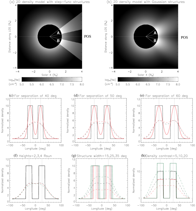
We synthesize $pB$ data for the west-limb region from 1.5 to 4 $R_{\odot}$ at longitudes in the range from $-90^{\circ}$ to 90^∘ using Equation (eqpb), and then derive the electron density using the SSPA method by fitting the synthetic $pB$ data. The panels (c)-(e) show comparisons of the SSPA density with the model density in the POS at 2 $R_{\odot}$ as a function of longitudes for different angular distances between two artificial structures with the density contrast ratio $d$=10. We find that for both types of the structure (in the step or Gaussian profile), the minimum resolvable distance (or angular resolution) is about 50^∘. To examine the effects of radial distance, structure width, and density contrast on the obtained resolution, we make a parametric study, and show the results in panels (f)-(h). We find that the resolution is only slightly dependent on the radial distance and structure width, which is better for the lower heights and narrower widths, but almost independent on the density contrast. In addition, we also find that the obtained SSPA peak density is about a half of the model density for the analyzed structures in most of the cases, which is consistent with our results for edge-on streamers. These numerical experiments suggest that for coronal structures with more smoothing profile and larger extension in the longitudinal direction and with lower density contrast to the background, which can be regarded as better conditions meeting the spherically symmetric assumption, the SSPA solutions are more accurate.

Acknowledgements

The work of TW was supported by the NASA Cooperative Agreement NNG11PL10A to the Catholic University of America and NASA grant NNX12AB34G. We very much appreciate to Dr. Maxim Kramar for his suggestions that led to an improved estimation of angular resolution of the SSPA method in Appendix. We also thank the anonymous referee for his/her valuable comments in improving the manuscript.

References

- Airapetian et al. (2011) Airapetian, V., Ofman, L., Sittler, E. C., Kramar, M.: 2011, ApJ 728, 67. DOI: 10.1088/0004-637X/728/1/67
- Allen (2000) Allen, C. W.: 2000, Allen’s Astrophysical Quantities (4th edition), Arthur N. Cox (ed.), Springer-Verlag, ISBN 0-387-98746-0.
- Barbey et al. (2008) Barbey, N., Auchére, F., Rodet, T., Vial, J.-C.: 2008, Sol. Phys. 248, 409. DOI: 10.1007/s11207-008-9151-6
- Barbey, Guennou, and Auchére (2013) Barbey, N., Guennou, C., Auchére, F.: 2013, Sol. Phys. 283, 227. DOI: 10.1007/s11207-011-9792-8
- Billings (1966) Billings, D. E.: 1966, A Guide to the Solar Corona, Academic Press, New York.
- Blackwell and Petford (1966a) Blackwell, D. E., Petford, A. D.: 1966a, MNRAS 131, 383. ADS: http://adsabs.harvard.edu/abs/1966MNRAS.131..383B
- Blackwell and Petford (1966b) Blackwell, D. E., Petford, A. D.: 1966b, MNRAS 131, 399. ADS: http://adsabs.harvard.edu/abs/1966MNRAS.131..399B
- Blackwell, Dewhirst, and Ingham (1967) Blackwell, D. E., Dewhirst, D. W., Ingham, M. F.: 1967, Advances in Astronomy and Astrophysics, Z. Kopal (ed.), New York, 5 1.
- Butala, Frazin, and Kamalabadi (2005) Butala, M. D., Frazin, R. A., Kamalabadi, F.: 2005, J. Geophys. Res. 110, A09S09. DOI: 10.1029/2004JA010938
- Butala et al. (2010) Butala, M. D., Hewett, R. J., Frazin, R. A., Kamalabadi, F.: 2010, Sol. Phys. 262, 495. DOI: 10.1007/s11207-010-9536-1
- Caroubalos et al. (2004) Caroubalos, C., Hillaris, A., Bouratzis, C., Alissandrakis, C. E., Preka-Papadema, P., Polygiannakis, J. et al.: 2004, A&A 413, 1125. DOI: 10.1051/0004-6361:20031497
- Cho et al. (2007) Cho, K.-S., Lee, J., Moon, Y.-J. Dryer, M., Bong, S.-C., Kim, Y.-H., Park, Y. D.: 2007, A&A 461, 1121. DOI: 10.1051/0004-6361:20064920
- Cranmer et al. (1999) Cranmer, S. R., Kohl, J. L., Noci, G., Antonucci, E., Tondello, G., Huber, M. C. E. et al.: 1999, ApJ 511, 481. DOI: 10.1086/306675
- Davila (1994) Davila, J. M.: 1994, ApJ 423, 871. DOI: 10.1086/173864
- Feng, Zhou, and Wu (2007) Feng, X. S., Zhou, Y. F., Wu, S. T.: 2007, ApJ 655, 1110. DOI: 10.1086/510121
- Frazin and Janzen (2002) Frazin, R. A., Janzen, P.: 2002, ApJ 570, 408. DOI: 10.1086/339572
- Frazin et al. (2007) Frazin, R. A., Vásquez, A. M., Kamalabadi, F., Park, H.: 2007, ApJ 671, L201. DOI: 10.1086/525017
- Frazin et al. (2010) Frazin, R. A., Lamy, P., Llebaria, A., Vásquez, A. M.: 2010, Sol. Phys. 265, 19. DOI:10.1007/s11207-010-9557-9
- Frazin et al. (2012) Frazin, R. A., Vásquez, A. M., Thompson, W. T., Hewett, R. J., Lamy, P., Llebaria, A., Vourlidas, A., Burkepile, J.: 2012, Sol. Phys. 280, 273. DOI: 10.1007/s11207-012-0028-3
- Gibson and Bagenal (1995) Gibson, S. E., Bagenal, F.: 1995, J. Geophys. Res., 100, 19865. DOI: 10.1029/95JA01905
- Gibson et al. (1999) Gibson, S. E., Fludra, A., Bagenal, F., Biesecker, D., del Zanna, G., Bromage, B.: 1999, J. Geophys. Res. 104, 9691. DOI: 10.1029/98JA02681
- Gopalswamy et al. (2003) Gopalswamy, N., Lara, A., Yashiro, S., Nunes, S. Howard, R. A.: 2003, Solar Variability as an Input to the Earth’s Environment, International Solar Cycle Studies (ISCS) Symposium, Wilson, A. (Ed.), ESA Publ. Division, Noordwijk, SP-535, 403.
- Groth et al. (2000) Groth, C. P. T., De Zeeuw, D. L., Gombosi, T. I., Powell, K. G.: 2000, J. Geophys. Res. 105, 25053. DOI: 10.1029/2000JA900093
- Guhathakurta and Fisher (1995) Guhathakurta, M., Fisher, R. R.: 1995, Geophys. Res. Lett. 22, 1841. DOI: 10.1029/95GL01603
- Guhathakurta, Holzer, and MacQueen (1996) Guhathakurta, M., Holzer, T. E., MacQueen, R. M.: 1996, ApJ 458, 817. DOI: 10.1086/176860
- Hayashi (2005) Hayashi, K.: 2005, ApJS 161, 480. DOI: 10.1086/491791
- Hayes, Vourlidas, and Howard (2001) Hayes, A. P., Vourlidas, A., Howard, R. A.: 2001, ApJ 548, 1081. DOI: 10.1086/319029
- Hu et al. (2008) Hu, Y. Q., Feng, X. S., Wu, S. T., Song, W. B.: 2008, J. Geophys. Res. 113, 3106. DOI:
- Kimura and Mann (1998) Kimura, H., Mann, I.: 1998, Earth Planets Space 50, 493. ADS: http://adsabs.harvard.edu/abs/1998EP
- Koutchmy (1994) Koutchmy, S.: 1994, Adv. Space Res. 14, 29. DOI: 10.1016/0273-1177(94)90156-2
- Koutchmy and Lamy (1985) Koutchmy, S., Lamy, P. L.: 1985, Properties and Interactions of Interplanetary Dust, R. H. Giese & P. L. Lamy (Eds.), ASSL 119, 63.
- Kramar et al. (2009) Kramar, M., Jones, S., Davila, J. M., Inhester, B., Mierla, M.: 2009, Sol. Phys. 259, 109. DOI: 10.1007/s11207-009-9401-2
- Kramar et al. (2011) Kramar, M., Davila, J., Xie, H., Antiochos, S.: 2011, Ann. Geophys. 29, 1019. DOI: 10.5194/angeo-29-1019-2011
- Kramar et al. (2013) Kramar, M., Inhester, B., Lin, H., Davila, J.: 2013, ApJ 775, 25. DOI: 10.1088/0004-637X/775/1/25
- Kramar et al. (2014) Kramar, M., Airapetian, V., Mikić, Z., Davila, J.: 2014,Sol. Phys., in press. DOI: 10.1007/s11207-014-0525-7
- Kwon et al. (2013) Kwon, R.-Y., Kramar, M., Wang, T. J., Ofman, L., Davila, J. M., Chae J.: 2013, ApJ 776, 55. DOI: 10.1088/0004-637X/776/1/55
- Lallement et al. (2010) Lallement, R., Quémerais, E., Lamy, P., Bertaux, J.-L., Ferron, S., Schmidt, W.: 2010, SOHO-23: Understanding a Peculiar Solar Minimum, S. R. Cranmer, J. T. Hoeksema, and J. L. Kohl. (eds.), ASP Conf. 428, 253.
- Lee et al. (2008) Lee, K.-S., Moon, Y.-J., Kim, K.-S., Lee, J.-Y., Cho, K.-S., Choe, G. S.: 2008, A&A 486, 1009. DOI: 10.1051/0004-6361:20078976
- Linker et al. (1999) Linker, J. A., Mikić, Z., Biesecker, D. A., Forsyth, R. J., Gibson, S. E., Lazarus, A. J. et al.: 1999, J. Geophys. Res. 104, 9809. DOI: 10.1029/1998JA900159
- Lionello, Linker, and Mikić (2009) Lionello, R., Linker, J. A., Mikić, Z.: 2009, ApJ 690, 902. DOI: 10.1088/0004-637X/690/1/902
- Manchester et al. (2004) Manchester, W. B., Gombosi, T. I., Roussev, I., de Zeeuw, D. L., Sokolov, I. V., Powell, K. G., Tóth, GáBor: 2004, J. Geophys. Res. 109, A02107. DOI: 10.1029/2003JA010150
- Manchester et al. (2005) Manchester, W. B., Gombosi, T. I., De Zeeuw, D. L., Sokolov, I. V., Roussev, I. I., Powell, K. G. et al.: 2005, ApJ 622, 1225. DOI: 10.1086/427768
- Mann (1992) Mann, I.: 1992, A&A 261, 329. ADS: http://adsabs.harvard.edu/abs/1992A
- Mikić et al. (1999) Mikić, Z., Linker, J. A., Schnack, D. D., Lionello, R., Tarditi, A.: 1999, Phys. Plasma 6, 2217. DOI: 10.1063/1.873474
- Minnaert (1930) Minnaert, M.: 1930, Zs. Ap. 1, 209. ADS: http://adsabs.harvard.edu/abs/1930ZA……1..209M
- Munro and Jackson (1977) Munro, R. H. Jackson, B. V.: 1977, ApJ 213, 874. DOI: 10.1086/155220
- November and Koutchmy (1996) November, L. J., Koutchmy, S.: 1996, ApJ 466, 512. DOI: 10.1086/177528
- Odstrčil and Pizzo (1999) Odstrčil, D., Pizzo, V. J.: 1999, J. Geophys. Res. 104, 493. DOI: 10.1029/1998JA900038
- Odstrčil et al. (2002) Odstrčil, D., Linker, J., Lionello, R., Mikić, Z., Riley, P., Pizzo, V. J., Luhmann, J. G.: 2002, J. Geophys. Res. 107, 1493. DOI: 10.1029/2002JA009334
- Quémerais and Lamy (2002) Quémerais, E. Lamy, P.: 2002, A&A 393, 295. DOI: 10.1051/0004-6361:20021019
- Quémerais et al. (2007) Quémerais, E., Lallement, R., Koutroumpa, D., Lamy, P.: 2007, ApJ 667, 1229. DOI: 10.1086/520918
- Ramesh et al. (2013) Ramesh, R., Kishore, P., Mulay, S. M., Barve, I. V., Kathiravan, C., Wang, T. J.: 2013, ApJ 778, 30. DOI: 10.1088/0004-637X/778/1/30
- Reames (1999) Reames, D. V.: 1999, Space Sci. Rev. 90, 41. DOI: 10.1023/A:1005105831781
- Riley, Linker, and Mikić (2001) Riley, P., Linker, J. A., Mikić, Z.: 2001, J. Geophys. Res. 106, 15889. DOI: 10.1029/2000JA000121
- Riley et al. (2006) Riley, P., Linker, J. A., Mikić, Z., Lionello, R., Ledvina, S. A., Luhmann, J. G.: 2006, ApJ 653, 1510. DOI: 10.1086/508565
- Saez et al. (2007) Saez, F., Llebaria, A., Lamy, P., Vibert, D.: 2007, A&A 473, 265. DOI: 10.1051/0004-6361:20066777
- Saito (1970) Saito, K.: 1970, Ann. Tokyo Astron. Obs., Ser. 2, 12, 53.
- Saito, Poland, and Munro (1977) Saito, K., Poland, A. I., Munro, R. H.: 1977, Sol. Phys. 55, 121. DOI: 10.1007/BF00150879
- Schulz (1973) Schulz, M. 1973, Ap&SS 24, 371. DOI: 10.1007/BF02637162
- Shen et al. (2013) Shen, C., Liao, C., Wang, Y., Ye, P., Wang, S.: 2013, Solar Phys. 282, 543. DOI: 10.1007/s11207-012-0161-z
- Sokolov et al. (2004) Sokolov, I. V., Roussev, I. I., Gombosi, T. I., Lee, M. A., Kóta, J., Forbes, T. G., Manchester, W. B., Sakai, J. I.: 2004, ApJ 616, L171. DOI: 10.1086/426812
- Thompson et al. (2010) Thompson, W. T., Wei, K., Burkepile, J. T., Davila, J. M., St. Cyr, O. C.: 2010, Sol. Phys. 262, 213. DOI:10.1007/s11207-010-9513-8
- Thompson (2006) Thompson, W. T.: 2006, A&A 449, 791. DOI: 10.1051/0004-6361:20054262
- Usmanov et al. (2000) Usmanov, A. V., Goldstein, M. L., Besser, B. P., Fritzer, J. M.: 2000, J. Geophys. Res. 105, 12675. DOI: 10.1029/1999JA000233
- Van de Hulst (1950) Van de Hulst, H. C.: 1950, Bull. Astron. Inst. Neth. 11, 135. ADS: http://adsabs.harvard.edu/abs/1950BAN….11..135V
- van der Holst et al. (2014) van der Holst, B., Sokolov, I. V., Meng, X., Jin, M., Manchester, W. B., IV, Tóth, G., Gombosi, T. I.: 2014, ApJ 782, 81. DOI: 10.1088/0004-637X/782/2/81
- Vásquez et al. (2008) Vásquez, A. M., Frazin, R. A., Hayashi, K., Sokolov, I. V., Cohen, O., Manchester, W. B., IV, Kamalabadi, F.: 2008, ApJ 682, 1328. DOI: 10.1086/589682
- Yashiro et al. (2004) Yashiro, S., Gopalswamy, N., Michalek, G., St. Cyr, O. C., Plunkett, S. P., Rich, N. B., Howard, R. A.: 2004, J. Geophys. Res. 109, 7105. DOI: 10.1029/2003JA010282
- Zucca et al. (2014) Zucca, P., Carley, E. P., Bloomfield, D. S., Gallagher, P. T.: 2014, A&A 564, 47. DOI: 10.1051/0004-6361/201322650