Indications of Intermediate-Scale Anisotropy of Cosmic Rays with
Energy Greater Than 57 EeV in the Northern Sky Measured
with the Surface Detector of the Telescope Array Experiment
Abstract
We have searched for intermediate-scale anisotropy in the arrival directions of ultrahigh-energy cosmic rays with energies above 57 EeV in the northern sky using data collected over a 5 year period by the surface detector of the Telescope Array experiment. We report on a cluster of events that we call the hotspot, found by oversampling using 20-radius circles. The hotspot has a Li-Ma statistical significance of 5.1, and is centered at , . The position of the hotspot is about 19 off of the supergalactic plane. The probability of a cluster of events of 5.1 significance, appearing by chance in an isotropic cosmic-ray sky, is estimated to be 3.710-4 (3.4).
1 Introduction
The origin of ultrahigh-energy cosmic rays (UHECRs), particles with energies greater than 1018 eV, is one of the mysteries of astroparticle physics. Greisen, Zatsepin, and Kuz’min (GZK) predicted that UHECR protons with energies greater than 60 EeV ( eV) would be severely attenuated primarily due to pion photoproduction interactions with the cosmic microwave background (CMB) radiation (Greisen, 1966; Zatsepin & Kuz’min, 1966). This GZK suppression becomes strong if these very high energy cosmic rays are produced at and traveling moderate extragalactic distances. The High Resolution Fly’s Eye (HiRes) collaboration was first to observe a suppression of cosmic rays above 60 EeV Abbasi et al. (2008), which is consistent with expectation from the GZK cutoff. This suppression was independently confirmed by both the Pierre Auger Observatory (PAO) (Abraham et al., 2008) in the south and Telescope Array (TA) experiment (Abu-Zayyad et al. 2013a, ) in the north, which are the largest aperture cosmic-ray detectors currently in operation.
The distribution of UHECR sources should be limited within the local universe with distances smaller than 100 Mpc for proton/iron and 20 Mpc for helium/carbon/nitrogen/oxygen (distances within which 50% of cosmic rays are estimated to survive) (Kotera & Olinto, 2011). To accelerate particles up to the ultrahigh-energy region, particles must be confined to the accelerator site for more than a million years by a magnetic field and/or a large-scale confinement volume (Hillas, 1984; Ptitsyna & Troitsky, 2010). This would thus limit the number of possible accelerators in the universe to astrophysical candidates such as galaxy clusters, supermassive black holes in active galactic nuclei (AGNs), jets and lobes of active galaxies, starburst galaxies, gamma-ray bursts, and magnetars. Galactic objects are not likely to be the sources since past observations indicate that the UHECRs do not concentrate in the galactic plane and have a relatively isotropic distribution. In addition, our galaxy cannot confine UHECRs above 1019 eV within its volume by the Galactic magnetic field. Extragalactic astrophysical objects form well-known large-scale structures (LSSs), most of which are spread along the “supergalactic plane” in the local universe. Nearby AGNs are clustered and concentrated around LSS with a typical clustering length of 5–15 Mpc, as observed by Swift BAT (Cappelluti et al., 2010). Concentrations of nearby AGNs coincide spatially with the LSS of matter in the local universe, including galaxy clusters such as Centaurus and Virgo. The typical amplitude of such AGN concentrations is estimated to be a few hundred percent of the averaged density within a 20-radius circle, which is of an angular scale comparable to the clustering length of the AGNs within 85 Mpc (Ajello et al., 2012).
The main difficulty in identifying the origin of UHECRs is the loss of directional information due to magnetic field induced bending. In order to investigate the UHECR propagation from the extragalactic sources, a number of numerical simulations have been developed (Yoshiguchi et al., 2003; Sigl et al., 2004; Takami et al., 2006; Kashti & Waxman, 2008; Koers & Tinyakov, 2009; Takami & Sato, 2010; Kalli et al., 2011; Takami et al., 2012). In the simulations, the UHECR trajectory between the assumed UHECR source and the Earth is traced through intergalactic and galactic magnetic fields (IGMF and GMF). The results depend strongly on the assumed distribution and density of the UHECR sources and the intervening magnetic fields. The deflection angle of a 60 EeV proton from a source at a distance of 50 Mpc is estimated to be a few degrees assuming models with an IGMF strength of 1 nG. Meanwhile, the estimated deflection by the GMF ranges from a few to about 10 degrees. This, however, depends on the direction in the sky. If the highest-energy cosmic rays come from the local universe such as nearby galaxies, and if they are protons, the maximum amplitude of the cosmic-ray anisotropy above 60 EeV is expected to be a few hundred percent of the average cosmic-ray flux. In this case, the amplitude of the cosmic-ray anisotropy might be detectable by the UHECR detectors of the TA and PAO.
In the highest-energy region, EeV, the PAO found correlations of the cosmic-ray directions within a 31-radius circle centered at nearby AGNs (within 75 Mpc) in the southern sky (Abraham et al., 2007). Updated measurements from the PAO indicate a weakened correlation with nearby AGNs (Abreu et al., 2010; Macolino, 2012); the correlating fraction (the number of correlated events divided by all events) decreased from the early estimate of ()% to ()%, compared with 21% expected for an isotropic distribution of cosmic rays. The chance probability of the original (69%) correlation is assuming an isotropic sky. The Telescope Array has also searched for UHECR anisotropies such as autocorrelations, correlations with AGNs, and correlations with the LSS of the universe using the first 40 months of scintillator surface detector (SD) data (Abu-Zayyad et al. 2012b, ; Abu-Zayyad et al. 2013b, ). Using 5 years of SD data, we updated results of the cosmic-ray anisotropy with EeV, which shows deviations from isotropy at the significance of 2–3 (Fukushima et al., 2013). In this letter, we report on indications of intermediate-scale anisotropy of cosmic rays with EeV in the northern hemisphere sky using the 5-year TA SD dataset.
2 Experiment
The Telescope Array is the largest cosmic-ray detector in the northern hemisphere. It consists of a scintillator surface detector (SD) array (Abu-Zayyad et al. 2012a, ) and three fluorescence detector (FD) stations (Tokuno et al., 2012). The observatory has been in full operation in Millard Country, Utah, USA (N, W; about 1,400 m above sea level) since 2008. The TA SD array consists of 507 plastic scintillation detectors each 3 m2 in area and located on a 1.2 km square grid. The array has an area of 700 km2. The TA SD array observes cosmic ray induced extensive air showers with 1 EeV, regardless of weather conditions with a duty cycle near 100% and a wide field of view (FoV). These capabilities ensure a very stable and large geometrical exposure over the northern sky survey in comparison with FD observations that have a duty cycle of 10%.
3 Dataset
In this analysis, we used SD data recorded between 2008 May 11 and 2013 May 4. The dataset contains approximately 1 million triggered events. For the reconstructed events, the energies determined by the SD array were renormalized by 1/1.27 to match the SD energy scale to that of the FD, which was determined calorimetrically (Abu-Zayyad et al. 2013a, ). Of these events, 72 met the following conditions: (1) each event included at least four SD counters; (2) the zenith angle of the event arrival direction was less than 55; and (3) the reconstructed energy was greater than 57 EeV, which corresponds to the energy threshold determined from the AGN correlation analysis results obtained by the PAO (Abraham et al., 2007), and is adopted here to avoid introducing a free parameter in the scanning phase space.
The event selection criteria above are somewhat looser than those of our previous analyses of cosmic-ray anisotropy (Fukushima et al., 2013) to increase the observed cosmic-ray statistics. In our previous analyses, the largest signal counter is surrounded by 4 working counters that are its nearest neighbours to maintain the quality of the energy resolution and angular resolution. Only 52 events survived those tighter cuts. When, the edge cut is abolished from the analysis (presented here) to keep more cosmic-ray events, 20 events with EeV are recovered compared with the tighter cut analysis. A full Monte Carlo (MC) simulation, which includes detailed detector responses (Abu-Zayyad et al. 2013a, ), predicted a 13.2 event increase in the number of events. The chance probability of the data increment being 20 as compared to the MC prediction of 13.2 is estimated to be 5%, which is within the range of statistical fluctuations. The angular resolution of array boundary events deteriorates to , compared to for the well contained events. The energy resolution of array boundary events also deteriorates to 20%, where that of the inner array events is 15%. These resolutions are still good enough to search for intermediate-scale cosmic-ray anisotropy. One final check is that when we calculate the cosmic ray spectrum using the loose cuts analysis, the result is consistent with our published spectrum.
4 Results
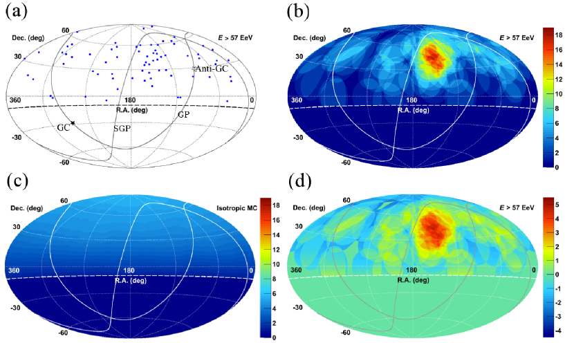
Figure 1 (a) shows a sky map in equatorial coordinates of the 72 cosmic-ray events with energy EeV observed by the TA SD array. A cluster of events appears in this map centered near right ascension 150, and declination 40, with a diameter of 30–40. In order to determine the characteristics of the cluster, and estimate the significance of this effect, we choose to apply elements of an analysis that was developed by the AGASA collaboration to search for large-size anisotropy (Hayashida et al. 1999a, ; Hayashida et al. 1999b, ), namely to use oversampling with a 20 radius. Being mindful that scanning the parameter space of the analysis causes a large increase in chance corrections, we have not varied this radius. The TA and HiRes collaborations used this method previously (Kawata et al., 2013; Ivanov et al., 2007) to test the AGASA intermediate-scale anisotropy results with their data in the 1018 eV range. The present letter reports on an extension of this method with application to the EeV energy region.
In our analysis, at each point in the sky map, cosmic ray events are summed over a 20-radius circle as shown in Figure 1 (b). The centers of tested directions are on a grid from to in right ascension (R.A.) and to in declination (Dec.). We found that the maximum of , the number of observed events in a circle of 20 radius is within the TA FoV. To estimate the number of background events under the signal in , we generated 100,000 events assuming an isotropic flux. We used a geometrical exposure as a function of zenith angle () because the detection efficiency above 57 EeV is 100%. The zenith angle distribution deduced from the geometrical exposure is consistent with that found in a full MC simulation. The MC generated events are summed over each 20-radius circle in the same manner as the data analysis, and the number of events in each circle is defined as . Figure 1 (c) shows the number of background events , where is the normalization factor.
We calculated the statistical significance of the excess of events compared to the background events at each grid point of sky using the following equation (Li & Ma, 1983):
| (1) |
Figure 1 (d) shows a significance map (in equatorial coordinates) of the events above 57 EeV as observed by the TA SD array. The maximum excess in our FoV appears as a “hotspot” centered at R.A.() , Dec.() with a statistical significance of ().
The significance of the hotspot, quoted above at 5.1, does not take random clustering into account, so one must make a correction. We did not carry out a blind analysis, but have been watching the hotspot grow over several years as we collected further data and added events to the sky plot. It is difficult to estimate the penalty due to our having seen the cluster of events. For example, in applying the oversampling technique used by the AGASA experiment, we knew the oversampling radius roughly matched the size of the hotspot cluster.
However, by making a simple MC calculation one can estimate the probability of such a hotspot appearing by chance anywhere in an isotropic sky. One generates many isotropic MC event sets, each with the statistics of the experimental data, then performs a calculation of the Li-Ma significance exactly as was done on the data; i.e., using oversampling with a radius of 20 degrees. One can go further and approximate the effect of the eye’s estimate of the radius of the cluster of events by repeating the calculation at other oversampling radii. We did this, choosing five oversampling radii, 15, 20, 25, 30, and 35 degrees. We chose a 5 degree scan since by eye one cannot make an estimate more accurately than about 5 degrees.
We generated 1 million MC data sets, each having 72 spatially random events within our FOV (i.e., we reproduced the statistics of the experimental data), assuming a uniform distribution over the TA SD exposure. The maximum of the significances, , was calculated for each MC dataset in the same way as in the data, with the exception that the five oversampling radii were used, and the largest was chosen. The distribution of the largest of the 1 million datasets is shown in Figure 2. We found that there were 365 instances of . This yields a chance probability of the observed hotspot in an isotropic cosmic-ray sky of 3.710-4, equivalent to a one-sided probability of 3.4.
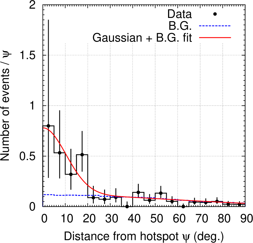
To estimate the size of the hotspot, we present (see Figure 3) the normalized number of events as a function of the opening angle, , relative to the center of the hotspot in the data. Although with current statistics we cannot determine the shape of the hotspot, to estimate its overall size we fit the hotspot excess using the binned maximum likelihood method, assuming a Gaussian signal plus a background estimated by the MC simulation. We used the following equation:
| (2) |
where the first term is the Gaussian signal, and and denote fitting parameters of the signal height and spread, respectively. The second term is the shape of the background fitted by a polynomial function determined from the MC simulations (, , and ). The spread of the hotspot was (). The uncertainty in the position of the hotspot is estimated to be .
5 Discussion
There are no known specific sources behind the hotspot. The hotspot is located near the supergalactic plane, which contains local galaxy clusters such as the Ursa Major cluster (20 Mpc from Earth), the Coma cluster (90 Mpc), and the Virgo cluster (20 Mpc). The angular distance between the hotspot center and the supergalactic plane in the vicinity of the Ursa Major cluster is 19.
Assuming the hotspot is real, two possible interpretations are: it may be associated with the closest galaxy groups and/or the galaxy filament connecting us with the Virgo cluster (Dolag et al., 2004); or if cosmic rays are heavy nuclei they may originate close to the supergalactic plane, and be deflected by extragalactic magnetic fields and the galactic halo field (Tinyakov & Tkachev, 2002; Takami et al., 2012). To determine the origin of the hotspot, we will need greater UHECR statistics in the northern sky. Better information about the mass composition of the UHECRs, GMF, and IGMF would also be important.
6 Summary
Using cosmic ray events with energy EeV, collected over 5 years with the TA SD, we have observed a cluster of events, which we call the hotspot, with a statistical significance of 5.1 (), centered at , . We calculated the probability of such a hotspot appearing by chance in an isotropic cosmic-ray sky to be 3.710-4 (3.4).
This indication of intermediate-scale anisotropy is limited by statistics collected by experiments in the northern hemisphere. It provides a strong impetus for an improved effort to study the origin of UHECRs. The TA4 project (extension of the TA SD by a factor of 4) (Sagawa et al., 2013) is designed to provide the equivalent of 20 TA-years of SD data by 2019, which would yield a 7 observation if the ratio of hotspot to background events remains as is currently seen. TA4 and other related projects will enable us to make a precise UHECR anisotropy map with high statistics and help solve the mystery of the UHECR origin.
Appendix A List of Events with EeV
In this Appendix we present the list of events with energy EeV and zenith angle that have been recorded by the surface detector of the Telescope Array from May 11, 2008 to May 4, 2013. During this period, 72 such events were observed. Table 1 shows the arrival date and time of these events, the zenith angle, energy in units of EeV, and equatorial coordinates (R.A.) and (Dec.) in degrees. Noted that the air shower reconstruction used here as described in Kawata et al. (2013) was slightly different from that of previous anisotropy work (Abu-Zayyad et al. 2012b, ). The opening angles between these arrival directions and previous ones are almost within 1. This difference hardly affects the results of the large-scale anisotropy.
References
- Abbasi et al. (2008) Abbasi, R. U., Abu-Zayyad, T., Allen, M., et al. 2008, Phys. Rev. Lett., 100, 101101
- Abraham et al. (2007) Abraham, J., Abreu, P., Aglietta, M., et al. 2007, Science, 318, 938
- Abraham et al. (2008) Abraham, J., Abreu, P., Aglietta, M., et al. 2008, Phys. Rev. Lett., 101, 061101
- Abreu et al. (2010) Abreu, P., Aglietta, M., Ahn, E. J., et al. 2010, Astropart. Phys., 34, 314
- (5) Abu-Zayyad, T., Aida, R., Allen, M., et al. 2012a, NIM-A, 689, 87
- (6) Abu-Zayyad, T., Aida, R., Allen, M., et al. 2012b, ApJ, 757, 26
- (7) Abu-Zayyad, T., Aida, R., Allen, M., et al. 2013a, ApJ, 768, L1
- (8) Abu-Zayyad, T., Aida, R., Allen, M., et al. 2013b, ApJ, 777, 88
- Ajello et al. (2012) Ajello, M., Alexander, D. M., Greiner, J., et al. 2012, ApJ, 749, 21
- Cappelluti et al. (2010) Cappelluti, N., Ajello, M., Burlon, D., et al. 2010, ApJ, 716, L209
- Dolag et al. (2004) Dolag, K., Grasso, D., Springel, V., & Tkachev, I. 2004, J. Korean Astron. Soc., 37, 427
- Fukushima et al. (2013) Fukushima, M., Ivanov, D., Kawata, K., et al. 2013, Proceedings of 33rd ICRC (Rio de Janeiro), CR-EX (Id:1033), in press
- Greisen (1966) Greisen, K. 1966, Phys. Rev. Lett., 16, 748
- (14) Hayashida, N., Nagano, M., Nishikawa, D., et al. 1999a, 26th ICRC (Salt Like CIty), OG1.3.04 (astro-ph/9906056)
- (15) Hayashida, N., Honda, K., Inoue, N., et al. 1999b, Astropart. Phys., 10, 303
- Hillas (1984) Hillas, A. M. 1984, ARA&A, 22, 425
- Ivanov et al. (2007) Ivanov, D., & Thomson, G.B. The HiRes Collaboration 2007, Proceedings of 30th ICRC (Merida), Ed. R. Caballero, et al. (Universidad Nacional Autonoma de Mexico, Mexico City, Mexico), 4, 445
- Kalli et al. (2011) Kalli, S., Lemoine, M., & Kotera, K. 2011, A&A, 528, 109
- Kashti & Waxman (2008) Kashti, T., & Waxman, E. 2008, J. Cosmology Astropart. Phys, 5, 6
- Kawata et al. (2013) Kawata, K., Fukushima, M., Ikeda, D., et al. 2013, Proceedings of 33rd ICRC (Rio de Janeiro), CR-EX (Id:311), in press
- Koers & Tinyakov (2009) Koers, H. B. J., & Tinyakov, P. 2009, J. Cosmology Astropart. Phys, 0904, 003
- Kotera & Olinto (2011) Kotera, K., & Olinto, A. V. 2011, ARA&A, 49, 119
- Li & Ma (1983) Li, T.-P., & Ma, Y.-Q. 1983, ApJ, 272, 317
- Macolino (2012) Macolino, C. 2012, J. of Phys.: Conf. Series, 375, 052002
- Ptitsyna & Troitsky (2010) Ptitsyna, K. V., & Troitsky, S. V. 2010, Phys. Uspekhi, 53, 691
- Sagawa et al. (2013) Sagawa, H., et al. 2013, Proceedings of 33rd ICRC (Rio de janeiro), CR-EX (Id:121), in press
- Sigl et al. (2004) Sigl, G., Miniati, F., & Ensslin, T. A. 2004, Phys. Rev. D, 70, 043007
- Takami et al. (2006) Takami, H., Yoshiguchi, H., & Sato, K. 2006, ApJ, 639, 803
- Takami & Sato (2010) Takami, H., & Sato, K. 2010, ApJ, 724, 1456
- Takami et al. (2012) Takami, H., Inoue, S., & Yamamoto, T. 2012, Astropart. Phys., 35, 767
- Tinyakov & Tkachev (2002) Tinyakov, P. G. & Tkachev, I. I. 2002, Astropart. Phys., 18, 165
- Tokuno et al. (2012) Tokuno, H., Tameda, Y., Takeda, M., et al. 2012, NIM-A, 676, 54
- Yoshiguchi et al. (2003) Yoshiguchi, H., Nagataki, S., Tsubaki, S., & Sato, K. 2003, ApJ, 586, 1211
- Zatsepin & Kuz’min (1966) Zatsepin, G. T., & Kuz’min, V. A. 1966, J. Exp. Theor. Phys. Lett., 4, 78

| Date and Time (UTC) | (deg) | (EeV) | (deg) | (deg) |
|---|---|---|---|---|
| 2008 Jun 10 17:05:37 | 46.91 | 88.8 | 93.50 | 20.82 |
| 2008 Jun 25 19:45:52 | 31.98 | 82.6 | 68.86 | 19.20 |
| 2008 Jun 29 08:22:45 | 41.20 | 101.4 | 285.74 | 1.69 |
| 2008 Jul 15 05:26:31 | 34.26 | 57.3 | 308.45 | 53.91 |
| 2008 Jul 20 04:35:32 | 25.61 | 120.3 | 285.46 | 33.62 |
| 2008 Aug 01 23:01:33 | 39.43 | 139.0 | 152.27 | 11.10 |
| 2008 Aug 09 06:16:16 | 14.54 | 76.9 | 280.28 | 41.34 |
| 2008 Aug 10 12:45:04 | 38.04 | 122.2 | 347.73 | 39.46 |
| 2008 Sep 24 20:09:22 | 23.16 | 68.8 | 178.03 | 20.29 |
| 2008 Oct 08 18:20:16 | 24.69 | 69.1 | 154.49 | 26.50 |
| 2008 Oct 30 17:30:35 | 27.45 | 79.3 | 152.44 | 45.84 |
| 2008 Nov 08 14:30:41 | 15.16 | 59.2 | 139.66 | 28.72 |
| 2008 Dec 30 10:49:32 | 4.11 | 59.7 | 152.30 | 36.45 |
| 2009 Jan 22 22:54:22 | 31.27 | 57.9 | 311.15 | 51.06 |
| 2009 Feb 12 01:00:17 | 41.63 | 64.2 | 22.49 | 80.07 |
| 2009 Mar 28 04:36:08 | 34.48 | 80.7 | 99.16 | 62.77 |
| 2009 Mar 29 03:43:34 | 20.84 | 75.0 | 119.62 | 59.19 |
| 2009 Apr 28 19:22:32 | 20.68 | 64.5 | 61.60 | 42.91 |
| 2009 May 19 02:19:52 | 42.51 | 64.2 | 206.74 | 24.93 |
| 2009 Jun 14 01:33:00 | 52.23 | 62.5 | 235.00 | 27.63 |
| 2009 Jul 13 04:38:52 | 40.41 | 154.3 | 239.85 | 0.41 |
| 2009 Aug 14 10:26:17 | 45.02 | 59.5 | 305.06 | 44.36 |
| 2009 Aug 15 08:54:55 | 23.27 | 65.2 | 331.65 | 18.85 |
| 2009 Sep 19 08:45:52 | 34.07 | 61.7 | 56.47 | 64.36 |
| 2009 Oct 21 10:49:42 | 4.38 | 66.5 | 82.19 | 43.12 |
| 2009 Nov 26 12:33:08 | 16.61 | 64.0 | 120.03 | 46.05 |
| 2010 Jan 08 07:17:31 | 19.04 | 57.6 | 128.77 | 44.51 |
| 2010 Jan 21 03:53:51 | 23.55 | 61.2 | 78.79 | 61.43 |
| 2010 Feb 22 07:10:34 | 11.58 | 63.7 | 139.13 | 49.62 |
| 2010 Feb 26 00:11:32 | 15.83 | 65.2 | 25.28 | 43.99 |
| 2010 Jul 11 03:01:45 | 44.90 | 58.0 | 212.37 | 4.78 |
| 2010 Jul 14 17:06:43 | 51.15 | 92.2 | 144.59 | 40.66 |
| 2010 Aug 05 19:44:07 | 45.54 | 67.1 | 115.13 | 1.45 |
| 2010 Aug 29 21:20:45 | 36.12 | 68.9 | 137.13 | 41.50 |
| 2010 Aug 30 20:50:45 | 19.60 | 93.5 | 204.00 | 45.18 |
| 2010 Sep 16 20:26:32 | 49.72 | 60.5 | 129.28 | 29.13 |
| 2010 Sep 19 07:05:00 | 23.66 | 66.3 | 19.29 | 32.26 |
| 2010 Sep 21 20:37:06 | 20.56 | 162.2 | 205.08 | 20.05 |
| 2011 Jan 05 00:56:23 | 8.93 | 67.4 | 359.91 | 31.47 |
| 2011 Jan 08 18:40:41 | 15.88 | 124.8 | 295.61 | 43.53 |
| 2011 Feb 28 16:16:26 | 38.94 | 135.5 | 288.30 | 0.34 |
| 2011 Apr 17 20:20:29 | 34.09 | 74.7 | 82.50 | 57.70 |
| 2011 Jul 13 19:12:34 | 42.73 | 65.4 | 87.59 | 81.53 |
| 2011 Jul 18 22:16:57 | 54.23 | 73.9 | 118.41 | 1.37 |
| 2011 Jul 22 22:15:41 | 10.64 | 62.3 | 163.67 | 28.92 |
| 2011 Jul 24 23:17:22 | 35.99 | 61.2 | 197.78 | 7.74 |
| 2011 Jul 28 15:21:08 | 19.18 | 89.3 | 39.98 | 34.17 |
| 2011 Aug 21 04:52:22 | 48.34 | 69.2 | 218.81 | 54.11 |
| 2011 Aug 25 22:05:12 | 23.98 | 83.3 | 168.48 | 57.92 |
| 2011 Aug 28 21:14:19 | 31.69 | 63.3 | 153.21 | 19.83 |
| 2011 Sep 10 21:16:00 | 44.24 | 78.8 | 133.62 | 48.55 |
| 2011 Oct 03 17:23:40 | 22.03 | 72.6 | 161.74 | 17.39 |
| 2011 Oct 21 06:33:06 | 15.71 | 78.7 | 31.32 | 49.49 |
| 2011 Oct 22 21:23:09 | 12.68 | 57.6 | 253.12 | 46.43 |
| 2011 Nov 09 16:51:22 | 24.30 | 72.9 | 156.84 | 38.82 |
| 2011 Nov 17 14:50:55 | 26.16 | 81.6 | 132.97 | 52.63 |
| 2011 Nov 19 22:39:41 | 38.07 | 57.4 | 319.95 | 15.87 |
| 2012 Jan 05 16:31:21 | 18.36 | 91.8 | 226.68 | 24.50 |
| 2012 Mar 13 02:54:54 | 25.25 | 60.3 | 123.94 | 22.52 |
| 2012 Apr 11 06:20:45 | 29.10 | 101.0 | 219.66 | 38.46 |
| 2012 May 04 00:18:13 | 24.42 | 76.9 | 134.84 | 59.83 |
| 2012 Aug 19 00:11:20 | 18.78 | 75.6 | 210.35 | 57.55 |
| 2012 Sep 07 22:30:26 | 38.79 | 57.8 | 158.60 | 60.26 |
| 2012 Sep 18 09:00:34 | 28.61 | 59.0 | 355.95 | 64.19 |
| 2012 Sep 27 13:51:05 | 45.68 | 57.4 | 159.75 | 35.56 |
| 2012 Nov 01 09:06:32 | 46.60 | 60.5 | 47.71 | 4.66 |
| 2013 Jan 03 09:56:20 | 54.73 | 68.2 | 66.42 | 39.00 |
| 2013 Mar 14 23:56:46 | 28.99 | 98.5 | 36.26 | 17.87 |
| 2013 Mar 21 22:45:18 | 26.91 | 106.8 | 37.59 | 13.89 |
| 2013 Apr 08 03:55:10 | 49.65 | 66.8 | 218.49 | 62.54 |
| 2013 Apr 22 01:13:31 | 36.20 | 62.5 | 165.28 | 52.35 |
| 2013 Apr 28 17:05:20 | 38.73 | 68.5 | 47.08 | 31.32 |
Note. — Table 1 is published in its entirety in the electronic edition of the Astrophysical Journal. A portion is shown here for guidance regarding its form and content.