AdS cycles in eternally inflating background

Abstract

In the eternally inflating background, the bubbles with AdS vacua will crunch. However, this crunch might be followed by a bounce. It is generally thought that the bubble universe may be cyclic, which will go through a sequence of AdS crunches, until the field inside bubble finally lands at a dS minimum. However, we show that due to the amplification of field fluctuation, the bubble universe going through AdS cycles will inevitably fragment within two or three cycles. We discuss its implication to the eternal inflation scenario.

I Introduction

During the eternal inflation [1], an infinite number of bubble universes with different dS and AdS vacua will spawn. The bubble universe with a dS minimum will arrive at a dS regime asymptotically, while the universe with AdS minimum will collapse rapidly. Inside an observational bubble universe, a phase of the slow-roll inflation and reheating is required, which will set the initial conditions of the “big bang” evolution, i.e. a homogeneous hot universe with the scale invariant primordial perturbation.

The slow roll inflation should occur in a high energy scale, which is required to insure that the amplitude of primordial perturbation is consistent with the observations and the reheating temperature is suitable for a hot big bang evolution after inflation. However, if the scale of the eternally inflating background is very low, the spawning of observational universe will be island-like, which is exponentially unfavored, since it requires a large upward tunneling, e.g. [2],[3],[4],[5],[6], and also [7],[8],[9] for an alternative study.

Recently, it has been argued that the nonsingular bounce in the eternally inflating background might significantly alter this result [10], and also [11],[12],[13],[14],[15]. In this scenario, the crunch of AdS bubble will be followed by a bounce, which makes the field inside bubble be able to finally land at a dS minimum, thus we actually may have a transition from AdS to dS [11],[14],[15]. The introduction of AdS bounce insures that the timelike geodesics in the eternally inflating spacetime dose not end at the big crunch singularity inside AdS bubbles, which may make the eternally inflating spacetime allow for a well-defined watcher measure [10], in which what is counted is the observations made by a single observer at a timelike geodesic, and also close related Refs.[2],[16]. In addition, AdS bounce also brings an efficient route to the slow-roll inflation. The bounce inflation may explain not only the power deficit on large angular scales, but also a large dipole power asymmetry in CMB [17],[18],[19] observed by the Planck collaboration, see also [20],[21],[22].

However, if the field inside bubble lands at a AdS minimum of its effective potential, the bubble universe will collapse and bounce again. Thus the bubble universe may go through a sequence of AdS crunches, during which it is cyclic, until the field inside bubble finally arrives at a dS minimum. Here, for convenience we call such a cyclic evolution as AdS cycles. Recently, the cosmological cyclic scenario, in which the universe goes through the periodic sequence of contraction and expansion [23], has been rewaked [24],[25],[26], which has leaded to significant insights for the origin of the observable universe. In Ref.[11], it is showed that during different cycles in cyclic universe, the universe may be in different vacua of a landscape, in which the inflation after bounce is responsible for the emergence of observational universe. In Ref.[27], it is showed that the inflation after bounce causes the cosmological hysteresis, which will lead to the increase of the amplitude of cycles. The cyclic or oscillating universe model also have been studied in Refs. [28],[29],[30],[31].

It is generally thought that the background of cyclic universe is homogeneous cycle by cycle all along. However, when the perturbation is considered, the case will be altered [12],[32], and also [33],[34]. The amplitude of curvature perturbation on large scale is increasing in the contracting phase, while it is almost constant in the expanding phase. Thus the net result of one cycle is that the amplitude of perturbation is amplified. This amplification of perturbation will be multiplied cycle by cycle, which will eventually lead that the homogeneity of background is destroyed.

Thus it is hardly possible that the AdS cycles of the bubble universe will continue all along until the field inside the bubble finally arrives at a dS minimum. How the amplification of perturbation affects the evolution of bubble universe in eternally inflating background is still interesting to study in details.

Recently, the amplification of field perturbation, which is induced by the self-interaction of field, has been studied in Ref.[14]. Here, we will concentrate on the amplification of field perturbation induced by the amplification of the curvature perturbation, which will generally arise when the bubble universe goes through AdS cycles.

We will show that due to the amplification of field fluctuation, the bubble universe going through AdS cycles will inevitably fragment within two or three cycles, and a number of new “bubble” universes will come into being from these fragments. In the eternally inflating scenario, compared to the nucleation of bubbles in dS background, the proliferation of bubble universe during AdS cycles is obviously more rapid, which will help the eternal inflation to more rapidly populate the whole landscape, wherever initially it happens.

II Review of AdS cycles in the landscape

We will firstly review the main result of the classical evolution of field during the AdS bounce, see also [11],[14],[15].

In eternally inflating background, the AdS bubble universe nucleated will inevitably collapse. The initial conditions of the bubble universe is set by the instanton. We follow [14]. Initially the bubble universe is in a phase dominated by the curvature $\rho_{Cur}\sim 1/a^{2}$, in which $a\sim t$ and $\phi$ is overdamped and approximately constant. When $t\sim 1/M_{\phi}$, the field $\phi$ begins to oscillate around its minimum with $\rho_{Mat}=\rho_{Mat0}/a^{3}$, which is equivalent to the matter with the state equation $w\simeq 0$. Here,

$$\rho_{Mat0}<\rho_{Cur}$$ (1)

is assumed. This implies that the evolution is approximately that of a AdS universe with the negative curvature,

$$a\simeq{1\over H_{\Lambda}}Sin\left(H_{\Lambda}t\right),$$ (2)

where $H_{\Lambda}=\sqrt{|\Lambda_{*}|\over 3}$ and $\Lambda_{*}$ is the depth of AdS minimum. The expansion ends at $t={\pi\over 2H_{\Lambda}}$ and is followed by the contraction dominated by $\rho_{Cur}$, i.e. the curvature phase. Before the bounce, the bubble universe may be still in a curvature phase, or a kinetic phase dominated by ${\dot{\phi}}^{2}$.

When the bounce scale is larger than the potential barrier, the field will be able to stride over the barrier. After the bounce, ${\dot{\phi}}^{2}\sim 1/a^{6}$ will be rapidly diluted and the field will eventually land at a different place of its effective potential. Thus the field $\phi$ will walk certain distance during the AdS bounce, i.e. one single AdS cycle. Here, “land” means that the effective potential of field begins to become dominated again. We define this displacement of $\phi$ as $\Delta\phi$, and have [11],[27]

$${\Delta\phi} \simeq {M_{P}\over\sqrt{6}}\ln({H_{B}^{4}\over H^{2}_{{Kin}}H^{2}_{{Land}}}),$$ (3)

where ‘Kin’ defines the beginning of the kinetic phase, which is the end of the matter contracting phase, and $H_{B}^{2}=\rho_{B}/3$ is defined. The result is consistent with that of Ref.[14]. We may assume $H_{{Kin}}\sim H_{{Land}}$, both which are generally smaller than $H_{B}$. Thus we have

$$\Delta\phi\gtrsim M_{P}.$$ (4)

During this period the number of hills and valleys the field flies over is determined by the detail of the landscape.

When the field lands at the dS minimum, the bubble universe will be in a dS state. However, if the field lands at a AdS minimum of its effective potential, the universe will collapse again, which will be followed by the AdS bounce again. The bubble universe may go through a sequence of AdS crunches, during which it is cyclic, called as AdS cycles, until the field finally lands at a dS minimum. In Appendix, a “toy” model of AdS cycles is introduced.

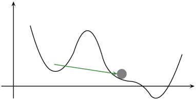
Figure 1: The sketch of an effective potential.

During the contraction of AdS cycles, the amplification of $\rho_{Mat}\sim 1/a^{3}$ is faster than $\rho_{Cur}$. When $\rho_{Mat}>\rho_{Cur}$, the bubble universe may be in a phase dominated by $\rho_{Mat}$, i.e. the matter contraction. We will see that the matter contracting phase is significant to rapidly amplify the perturbation. However, when $\rho_{Mat}\sim\rho_{Mat0}$, we have $H\sim M_{\phi}$, which implies the oscillating phase ends. Thus it seems hardly possible that we have the matter contracting phase in the $1^{th}$ cycle [14].

However, after the $1^{th}$ cycle the initial conditions of the field evolution will be set not by the instanton, but by the details of previous cycle. In this case, the oscillating energy $\rho_{Mat}$ of field will may be large, thus we may have the matter contracting phase in the cycles after the $1^{th}$ cycle.

However, we may also have the matter contracting phase in the $1^{th}$ cycle when relaxing the assumption (1). In Fig.1, we plot a potential, for which after the bubble nucleates, the field may be placed in a plain of its potential. In this case, the bubble universe may has a short inflationary phase, which will rapidly dilute $\rho_{Cur}$. Hereafter, the field rolls toward AdS minimum, and begins to oscillate around it. The evolution will be that of a AdS universe with the oscillating energy $\rho_{Mat}$.

It is generally thought that the AdS cycles will continue all the time until the bubble universe finally “transits” to a dS state. However, if the perturbation of field is considered, the scenario will be altered.

III The proliferation of bubble universe

III.1 Amplification of perturbations through cycles

We will investigate the evolution of the scalar field perturbation through cycles. Here, the mode spectrum of the perturbation may involve some supercurvature modes, see e.g.[35],[36]. However, for simplicity, we will only concentrate on modes whose initial wavelength is smaller than the radius of curvature, and also on almost flat case. In this case, the calculation of the perturbation may be similar to that in flat case.

In the perturbation equation of scalar field $\phi$, the terms ${\dot{\phi}}{\dot{\Phi}}$ and $\Phi{\partial V\over\partial\phi}$, coupling to the metric perturbation $\Phi$, should be not negligible during the contraction, since both $\dot{\phi}$ and $\Phi$ are rapidly increasing. The equations of perturbations are a set of coupling equations between $\Phi$ and $\delta\phi$, thus solving the equation of $\delta\phi$ has to simultaneously solve the equation of the metric perturbation, which will complicate the calculations. However, noting that the field perturbation is related to the comoving curvature perturbation ${\cal R}$

$${H\over\dot{\phi}}\delta{\phi}={\cal R}-\Phi,$$ (5)

thus we might firstly calculate ${\cal R}$ and then apply Eq.(5) to obtain $\delta\phi$. The equation of $\cal R$ in momentum space is [37],[38]

$$u_{k}^{\prime\prime}+\left(k^{2}-{z^{\prime\prime}\over z}\right)u_{k}=0,$$ (6)

after $u_{k}\equiv z{\cal R}_{k}$ is defined, where ^′ is the derivative with respect to the conformal time $\eta=\int dt/a$, $z\equiv a\sqrt{2M_{P}^{2}\epsilon}$ and $\epsilon=-{\dot{H}}/H^{2}$.

When $k^{2}\simeq z^{\prime\prime}/z$, the perturbation mode is leaving the horizon. When $k^{2}\ll z^{\prime\prime}/z$, the solution of $\cal R$ given by Eq.(6) is

$${\cal R}_{k} \sim C\,\,\,\,\,is\,\,\,{{\rm constant}}\,\,\,{{\rm mode}}$$ (7)

$$or \,D\int{d\eta\over z^{2}}\,\,\,\,\,is\,\,\,{{\rm decaying/growing}}\,\,\,{{\rm mode}},$$ (8)

where the $D$ mode is decaying or growing is dependent on the behavior of $z$.

The contraction phase may be regarded as

$$a\sim(t_{B}-t)^{n},$$ (9)

where $t<t_{B}$ is negative, and the parameter $n$ is constant, which is set only for the convenience of discussion. Thus during the contraction with $n>{1\over 3}$, the amplitude of $\cal R$ will be dominated by the growing mode,

$${\cal R}_{k}\sim\int{d\eta\over z^{2}}\sim\left(t_{B}-t\right)^{1-3n}.$$ (10)

In principle, ${\cal R}_{k}$ will increase up to the end of this contracting phase.

The amplitude of growing mode before the bounce may inherited by the constant mode after the bounce [39], [40],[41], which is actually the requirement that the curvature perturbation continuously comes through the bounce. While in the expanding phase, the constant mode is dominated, thus ${\cal R}_{k}$ will be unchanged until the beginning of next contraction.

We will regard the beginning time of contracting phase as the beginning of a cycle, and in one single cycle the universe will orderly experience the contraction, bounce and expansion. In the $j^{th}-1$ cycle, after the bounce, we have ${\cal R}_{k}^{j-1}$, which will be constant up to the beginning of the $j^{th}$ cycle. During the contraction of the $j^{th}$ cycle, ${\cal R}_{k}^{j}$ will continue to increase. Thus after the bounce of the $j^{th}$ cycle, we have

$${\cal R}_{k}^{j}(t^{j}) \simeq \left(\frac{t_{B}^{j}-t^{j}}{t_{B}^{j}-t_{Ci}^{j}}\right)^{1-3n_{j}}{\cal R}_{k}^{j-1}(t_{Ce}^{j-1})$$ (11)

$$\sim \prod_{l=2}^{j}\left(\frac{t_{B}^{l}-t^{l}}{t_{B}^{l}-t_{Ci}^{l}}\right)^{1-3n_{l}}{\cal R}_{k}^{1}(t_{Ce}^{1}),$$

where $t_{Ci}^{j}$ and $t_{Ce}^{j}$ are the beginning time and the end time of contracting phase in the $j^{th}$ cycle, respectively. Here, we only consider the perturbation mode, which is still outside the horizon all along after it leaves the horizon in the $1^{th}$ cycle, or see the details in Ref.[32].

The metric perturbation satisfies $({a\Phi_{k}\over H})^{.}=a{\cal R}_{k}\epsilon$, e.g.[42], thus we have $a\Phi_{k}/H=\int^{t}a{\cal R}_{k}\epsilon\,\,dt^{\prime}$. The perturbation $\delta\phi$ of $\phi$ may be calculated as

$$\delta\phi_{k} = \sqrt{2M_{P}^{2}\epsilon}{\cal R}_{k}\left(1-{{H\over a}\int^{t}a{\cal R}_{k}\epsilon\,\,dt^{\prime}\over{\cal R}_{k}}\right)\simeq\sqrt{2M_{P}^{2}\epsilon}{\cal R}_{k}$$ (12)

$$\sim \left(t_{B}-t\right)^{1-3n},$$

where we have ${H\over a}\int^{t}a{\cal R}_{k}\epsilon\,\,dt^{\prime}\sim{\cal R}_{k}$ in light of Eqs.(9) and (10), which implies that the perturbation $\delta\phi$ of field will increase synchronously with ${\cal R}_{k}$. Thus we have

$$\phi_{k}^{j}(t^{j}) \simeq \left(\frac{t_{B}^{j}-t^{j}}{t_{B}^{j}-t_{Ci}^{j}}\right)^{1-3n_{j}}{\phi}_{k}^{j-1}(t_{Ce}^{j-1})$$ (13)

$$\sim \prod_{l=2}^{j}\left(\frac{t_{B}^{l}-t^{l}}{t_{B}^{l}-t_{Ci}^{l}}\right)^{1-3n_{l}}{\phi}_{k}^{1}(t_{Ce}^{1}).$$

Both Eqs.(11) and (13) indicates that the perturbation will be multipled through cycles, and thus the rate of the amplification is quite rapid.

We plot the evolutions of $\delta\phi$ in Figs.2 and 3 by numerically solving the set of the coupling equations of $\Phi$ and $\delta\phi$, e.g.[43]. We can clearly see that $\delta\phi$ is increasing during the contraction and is almost constant during the expansion, thus the net result is that the amplitude of perturbation is multipled through cycles, which is consistent with Eq.(13).

Here, we have assumed that the linear perturbation approximation is satisfied all along. However, we will obviously see that it will be broken in the $j^{th}_{Cutoff}$ cycles, which will set a cutoff for the number of times of the AdS cycles of bubble universe.

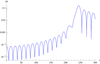
Figure 2: The evolution of $\delta\phi$ with respect to the time for the potential in the upper panel of Fig.7. The field goes through one single AdS cycle, and its perturbation increases during the corresponding contracting phase.

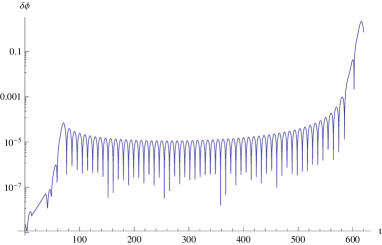
Figure 3: The evolution of $\delta\phi$ with respect to the time for the potential in the lower panel of Fig.7. The field goes through two AdS cycles, and its perturbation increases during the contracting phase of each AdS cycle.

III.2 Fragment of bubble universe

We will estimate the value of $j_{Cutoff}$, in which cycle ${\cal P}_{\cal R}\sim 1$ is arrived at.

During the contraction of AdS cycles, the universe will come through the matter contracting phase, the kinetic phase and arrive at the bounce. The perturbation amplitude will be amplified in the matter contracting phase, in which

$${\cal R}_{k}\sim{1\over t_{B}-t},$$ (14)

see Eq.(10). The amplification of the perturbation amplitude in kinetic phase is

$${\cal R}_{k}\sim\int{d\eta\over z^{2}}\sim\ln(t_{B}-t),$$ (15)

which is negligible, compared with that in matter contracting phase. In curvature phase, since $a\sim 1/H$, the perturbation mode initially inside the horizon will be still inside the horizon, which thus will not be amplified. In addition, during the bounce the perturbation is not also amplified [44].

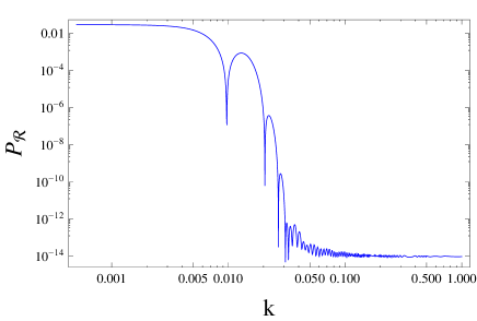
Figure 4: The snapshot of the power spectrum of curvature perturbation in the $2^{th}$ AdS cycle with the evolution of the background field in Fig.10.

When $k^{2}\gg z^{\prime\prime}/z$, the perturbation is deep inside its horizon, $u_{k}$ oscillates with a constant amplitude. The initial value is

$$u_{k}\sim{1\over\sqrt{2k}}e^{-ik\eta}.$$ (16)

When $k^{2}\ll{z^{\prime\prime}\over z}$, the perturbation is far outside its horizon, the solution of Eq.(6) can be obtained, which gives

$${\cal P}_{\cal R}^{1/2}={k^{3/2}\over\sqrt{2\pi^{2}}}\left|{\cal R}_{k}\right|\sim{H_{Kin}\over\sqrt{\epsilon_{Mat}}M_{P}},$$ (17)

where ${\cal R}_{k}={u_{k}/z}$ is used. The spectrum is scale invariant [45],[46]. This is the perturbation spectrum after the bounce in the $1^{th}$ cycle. Thus in the $j^{th}$ cycle, ${\cal P}_{\cal R}$ on the corresponding scale is given by

$${\cal P}_{\cal R}^{1/2}={k^{3/2}\over\sqrt{2\pi^{2}}}\left|{\cal R}^{j}_{k}\right|\sim\left(\prod_{l\,\,=\,\,2}^{j}{H^{l}_{Kin}\over H^{l}_{*}}\right){H^{1}_{Kin}\over\sqrt{\epsilon_{Mat}}M_{P}},$$ (18)

where Eq.(14) and $H\sim{1/(t_{B}-t)}$ are used, and $H_{*}$ is the Hubble parameter at the beginning time of the matter contracting phase. We may assume, for simplicity, that $H_{Kin}$ in all cycles are equal, as well as $H_{*}$, which makes Eq.(18) becomes

$${\cal P}_{\cal R}^{1/2}\sim\left({H_{Kin}\over H_{*}}\right)^{j}{H_{*}\over\sqrt{\epsilon_{Mat}}M_{P}}.$$ (19)

Thus the breaking of the linear perturbation approximation ${\cal P}_{\cal R}^{1/2}\gtrsim 1$ implies

$$j_{Cutoff}\gtrsim{\ln^{-1}\left({H_{Kin}\over H_{*}}\right)\ln{\sqrt{\epsilon_{Mat}}M_{P}\over H_{*}}}.$$ (20)

This result implies that the larger the ratio between the scales that the matter contracting phase begins and ends is, i.e. ${H_{Kin}/H_{*}}$, the smaller $j_{Cutoff}$ is. When $j_{Cutoff}=1$, we have

$$H_{Kin}\sim M_{P},$$ (21)

which is consistent with Eq.(17). Thus unless the bounce occurs in Planck scale, it is hardly possible that in the $1^{th}$ cycle the amplitude of curvature perturbation increases up to 1. When

$${H_{Kin}\sim H_{*}},$$ (22)

we may have $j_{Cutoff}\gg 1$, which, however, is still a finite number. Here, (22) is equivalent with the condition that the ratio of the maximal value of $a$ to its minimal one is ${\cal O}(1)$ in Ref.[33]. In certain sense, the increase of the perturbation amplitude means that an infinite cycles is impossible.

When $j_{Cutoff}=2$, we have

$$H_{*}\lesssim\left({H_{Kin}\over M_{P}}\right)H_{Kin}.$$ (23)

Thus $H_{*}$ has to be large, or ${\cal P}_{\cal R}^{1/2}\sim 1$ will be arrived in this cycle. When ${H_{Kin}\over M_{P}}\sim 10^{-5}$, which is often required by the bouncing model in which the observable universe may appear after one single bounce, we have $H_{*}\lesssim 10^{-5}H_{Kin}$, which seems easily satisfied. Thus it seems highly possible that ${\cal P}_{\cal R}^{1/2}\sim 1$ will occur at $j=2$.

We could reestimate this observation in light of the details of the landscape. Here, $H_{Kin}$ is defined when ${\dot{\phi}}^{2}$ begins to dominate, i.e. ${{\dot{\phi}}^{2}}\sim{V_{Bar}}$, which gives $H^{2}_{Kin}\sim{V_{Bar}\over M_{P}^{2}}$, in which $V_{Bar}$ is the barrier separating different minima of effective potential. While when the matter contracting phase begins, we have $\rho_{Mat}\sim\rho_{Cur}\gtrsim{|{\Lambda}_{*}|}$, which gives $H^{2}_{*}\gtrsim{|{\Lambda}_{*}|\over M_{P}^{2}}$. Thus Eq.(18) becomes

$${\cal P}_{\cal R}^{1/2} \lesssim \left(\prod_{l\,\,=\,\,2}^{j}\sqrt{V^{l}_{Bar}\over|{\Lambda}^{l}_{*}|}\right){\sqrt{V^{l}_{Bar}}\over\sqrt{\epsilon_{Mat}}M_{P}}$$ (24)

$$= \left({V_{Bar}\over|{\Lambda}_{*}|}\right)^{j/2}{\sqrt{\Lambda}_{*}\over\sqrt{\epsilon_{Mat}}M_{P}},$$

where in the second line we assume that $V_{Bar}$ in all cycles are equal, as well as ${\Lambda}_{*}$. When $j_{Cutoff}=2$, we have

$$|{\Lambda}_{*}|<\left({V_{Bar}\over M_{P}^{4}}\right)V_{Bar},$$ (25)

where $|{\Lambda}_{*}|$ is the depth of AdS minimum in a landscape, see also the effective potential (32). We see that if ${V_{Bar}^{1/4}\over M_{P}}\sim 10^{-3}$, $|{\Lambda}_{*}|^{1/4}>10^{-3}V_{Bar}^{1/4}$ has to be required for avoiding ${\cal P}_{\cal R}^{1/2}\sim 1$ in this cycle. Thus we may conclude that for a high potential barrier $V_{Bar}$, unless AdS minimum is far deep, generally we have $j_{Cutoff}=2$, i.e. ${\cal P}_{\cal R}^{1/2}\sim 1$ will be rapidly arrived within two cycles.

We numerically show the change of the power spectrum ${\cal P}_{\cal R}$ through AdS cycles in Fig.4 with the evolution of the background field in Fig.10. The power spectrum ${\cal P}_{\cal R}^{1}$ after the bounce in the $1^{th}$ cycle is scale invariant, which is given by a long period of the matter contraction. During the contraction of the $2^{th}$ cycle, the shape of spectrum on large scale is unchanged, i.e. still scale invariant, but its amplitude is amplified. The spectrum on small scale is also scale invariant, since the corresponding modes are newly generated in the $2^{th}$ cycle. The spectrum of the modes on middle scale will redshift. The result is consistent with Eq.(18).

When ${\cal P}_{\cal R}^{1/2}\sim 1$, it is hardly possible that the background inside the bubble universe is still homogeneous. The effect of the perturbation on background is plotted in Fig.5 by transforming ${\cal R}_{k}$ into ${\cal R}(\vec{x})$ in position space. We see that in the $2^{th}$ cycle, the increase of the perturbation will eventually make the initially homogeneous background become highly inhomogeneous, i.e. fragment, thus the global cycle of the universe will inevitably terminate.

Here, the existence of the matter contracting phase is crucial for the amplification of perturbation. Thus based on the discussions in II, we may conclude that the bubble universe going through AdS cycles will become highly inhomogeneous, or fragment, within two or three cycles, dependent on the details of landscape.

Figure 5: ${\cal R}(\vec{x})$ in position space, which reflects the inhomogeneity of background when ${\cal P}_{\cal R}\sim 1$ on large scale.

III.3 New “bubble” universes after fragment

We have showed that the bubble universe going through AdS cycles will fragment at certain time $t_{Frag}$ within the $2^{th}$ or $3^{th}$. We will see what is the resulting scenario.

The average square of the amplitude of field fluctuations at $t_{Frag}$ is

$$<\delta\varphi^{2}_{k}>={1\over(2\pi)^{3}}\int\left|\delta\varphi_{k}\right|^{2}d^{3}k$$ (26)

$$\simeq {1\over(2\pi)^{3}}\int^{aH}_{aH/e}3M_{P}^{2}\left(1-{{H\over a}\int^{t}a{\cal R}_{k}\epsilon_{Mat}\,\,dt^{\prime}\over{\cal R}_{k}}\right)^{2}\left|{\cal R}_{k}\right|^{2}d^{3}k$$

$$= 3M_{P}^{2}\,/4.$$

where $2\epsilon_{Mat}M_{P}^{2}=3M_{P}^{2}$ for the matter contraction and ${\cal P}_{\cal R}\sim 1$ are used. Thus at this moment it is inevitable that the fields in different causal regions with length $1/H_{Frag}$ will randomly jumps, in which $H_{Frag}={1\over t_{B}-t_{Frag}}$ is the Hubble parameter at $t_{Frag}$, which generally satisfies $H_{*}\ll H_{Frag}<H_{Kin}$.

When $t=t_{Frag}$, we have approximately

$${\cal P}_{\cal R}^{1/2}\sim{H_{Frag}\over H_{*}}{H_{Kin}\over\sqrt{\epsilon_{Mat}}M_{P}}\sim 1.$$ (27)

When the matter contraction begins, i.e. $t=t_{*}$, the length $l_{*}$ of the homogeneous region inside the bubble should at least satisfy $l_{*}\gtrsim 1/H_{*}$. Thus noting $l\sim a\sim(t_{B}-t)^{2/3}$ and $H\sim 1/(t_{B}-t)$, at $t_{Frag}$ we have

$$\left({l_{Frag}\over 1/H_{Frag}}\right)^{3}\simeq{H_{Frag}\over H_{*}}\sim{\sqrt{\epsilon_{Mat}}M_{P}\over H_{Kin}}\gg 1,$$ (28)

where Eq.(27) is used. Thus at $t_{Frag}$, initial homogeneous region will include lots of local regions with length $1/H_{Frag}$.

It is conceivable that in different local regions with the radius $l_{Local}>1/H_{Frag}$, the field will jump to a different place of its effective potential. In some regions, the field jumps to certain place of its effective potential, which leads to $\rho_{Local}>\rho_{Frag}$, thus

$${1/H_{Local}}<{1/H_{Frag}}<l_{Local},$$ (29)

in which $1/H_{Local}$ is the Hubble length of the corresponding region. This implies that the trapped surface has got formed inside these regions. In this sense, such a region actually corresponds to a new “bubble” universe and will continue to its contracting phase therein. While in other regions we might have $\rho_{Local}<\rho_{Frag}$, i.e. $1/H_{Local}>1/H_{Frag}$ thus initially there is not the trapped surface. However, since the correspond region is contracting, $1/H_{Local}$ will shrink and ultimately become same order with $1/H_{Frag}$, at this time the trapped surfaces also can get formed.

Thus the initial bubble universe will fragment into a number of local regions separated by domain walls, each of which actually corresponds to a new “bubble” universe. We may visually call this as the proliferation of bubble universe. These “bubble” universes after proliferation will continue to go through cycles and then fragment into newer “bubble” universes until the field in corresponding bubble lands at certain dS minimum.

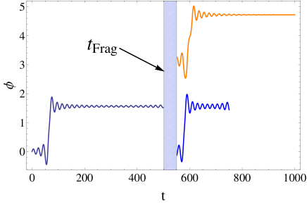
Figure 6: The possible evolutions of fields inside different “bubble” universes after the fragment, based on Fig.10 for the effective potential in the lower panel of Fig.7. The initial conditions of evolutions for them are that at $t=t_{Frag}$ the value of field is shifted $\sqrt{<\delta\varphi^{2}_{k}>}\sim 1\,\phi_{Unit}$ but $\dot{\phi}$ and the sign of $\dot{a}$ are not altered. In Fig.10 the field will go through two AdS cycles and eventually land at the $\phi\simeq 3\phi_{Unit}$. However, if the effect of the field fluctuation is considered, the case will be altered, the field with $+\phi_{Unit}$ shift will eventually land at the $\phi\simeq 5\phi_{Unit}$, while the field with $-\phi_{Unit}$ shift will eventually land at the $\phi\simeq 1.5\phi_{Unit}$. Here, $t$ is the global cosmic time, however, after $t_{Frag}$, in principle each local region, or universe, has itself clock.

We plot the possible evolutions of fields inside the new “bubble” universes in Fig.6, based on Fig.10 with the assumption that at $t=t_{Frag}$ the value of field is shifted $\sqrt{<\delta\varphi^{2}_{k}>}$, but $\dot{\phi}$ and the sign of $\dot{a}$ are not changed. Here, $t$ is the global cosmic time, however, after $t_{Frag}$, in principle each universe has itself clock.

In Fig.10, the effect of the field fluctuation is not considered, the field will go through two AdS cycles and eventually lands at the dS minimum. However, in Fig.6, the case is altered, the global universe will fragment within two AdS cycles, and after the fragment the evolutions of fields inside different “bubble” universes will be different, after the bounce the field with the shift $-\sqrt{<\delta\varphi^{2}_{k}>}$, or jumping back, will land at the AdS minimum again, and the corresponding universe will begin next cycle and might proliferate again, while the field with the shift $+\sqrt{<\delta\varphi^{2}_{k}>}$, or jumping forward, will land at a more distant part of the potential landscape, which might be a dS minimum, as in Fig.6, and might not. Thus after the proliferation the experiences of different “bubble” universes is not generally different, when some universes are in a phase of the matter contraction, other universes might be in the phase of the inflationary expansion or bounce.

It is also noted that the classical displacement of field during one single cycle is approximately given by Eq.(4), thus we have

$${\sqrt{<\delta\varphi^{2}_{k}>}\over\Delta\varphi}={{3\over\sqrt{2}}\ln^{-1}\left({H_{B}^{4}\over H^{2}_{{Kin}}H^{2}_{{Land}}}\right)}\sim 0.1-1.$$ (30)

This result indicates that when ${\cal P}_{\cal R}^{1/2}\sim 1$ the fluctuation of field will be close to the order of its classical displacement during one single cycle. In certain sense, this might provide an alternative insight to the conclusion that the AdS bubble universe will fragment within two or three cycles.

IV Discussion

We have showed that in eternally inflating background, due to the amplification of field fluctuation, the bubble universe going through AdS cycles will inevitably fragment within two cycles or three cycles and a number of new “bubble” universes with different vacua will come into being from these fragments. This proliferation helps the eternal inflation to more rapidly populate the whole landscape, in whichever corner of landscape it initially happens.

How to assign probabilities to different events in the eternally inflating multiverse has been still a significant issue, e.g.[47] for a review. The watcher measure [10], in which all timelike geodesics are required to extend to infinity, might be a promising avenue to address the relevant problem. Our result solidifies the background of the watcher measure, in which different regions of AdS bubble may “transit” to different vacua.

It is conceivable that a phase of slow-roll inflation might occur after the bounce. The bounce inflation may fit the observations well, e.g.[17],[18], which is interesting for studying. We will back to this issue in details elsewhere.

Recently, it has been argued [48] that with AdS bounce, the eternally inflating background is still past-incomplete. However, with the proliferation of bubble universe, it might be interesting to relook through this argument.

Acknowledgments

This work is supported in part by NSFC under Grant No:11222546, and in part by National Basic Research Program of China, No:2010CB832804.

Appendix: A “toy” model of AdS cycles

We will introduce a “toy” model of AdS cycles, which will be used to simulate the evolution of perturbation in Sec. III and IV. The Lagrangian is

$$\mathcal{L}=\frac{1}{2}\partial_{\mu}\phi\partial^{\mu}\phi-\left(\frac{1}{2}\partial_{\mu}\psi\partial^{\mu}\psi\right)^{2/3}-V(\phi).$$ (31)

Here, we regard the potential as

$$V=V_{Bar}\left(1-\cos({M_{\phi}\over\sqrt{V_{Bar}}}\phi)\right)-{\Lambda}_{*}\cos({M_{\phi}\over N_{Int}\sqrt{V_{Bar}}}\phi+\theta),$$ (32)

which may be the axion field in string theory, e.g.[49],[50], where we require that ${\Lambda}_{*}\ll V_{Bar}$ and $N_{Int}>0$ is the integer. This potential has periodic minimal values, in which $V_{Bar}$ sets the height of the potential barrier and ${\Lambda}_{*}$ sets the depth of AdS minimum. When $N_{Int}=2$, the potential around $\phi=0$ is approximately

$$V\simeq{M_{\phi}^{2}\phi^{2}\over 2}-{\Lambda}_{*},$$ (33)

which is AdS-like, while around its adjacent minimum, i.e. $\phi_{1}={2\pi\sqrt{\Lambda_{*}}\over M_{\phi}}$, the potential is approximately

$$V\simeq{M_{\phi}^{2}(\phi-\phi_{1})^{2}\over 2}+{\Lambda}_{*},$$ (34)

which is dS-like. Thus in this potential the dS minimum and the AdS minimum alternate, see the upper panel in Fig.7. While when $N_{Int}=\,4$ and $\theta={\pi/\,4}$, we have a potential in which two AdS minima and two dS minima alternate, see the lower panel in Fig.7.

The bounce is induced by the evolution of field $\psi$, which is ghostlike. Here, we will regard $\psi$ as a purely classical field to implement the background evolution of the nonsingular bounce [39], which is only significant around the bounce and otherwise negligible.

However, it is generally thought that the appearance of such a field is only the approximation of a fundamental theory below certain physical cutoff. e.g. see G-bounce [51],[52],[53],[54] and super-bounce [55], and also [57] for a review. The bounce is also implemented in e.g.[58] for Pre-big bang scenario, [56] for ekpyrotic scenario, and also the string-inspired gravity [59],[60], the multiscale gravity [61], other modified gravity [62], see [63],[64] for reviews.

The bounce generally occurs in a high energy scale, thus the relevant physics are only reflected on the perturbation modes at far small scale, while the perturbation modes which we care are those at far large scales. Thus for different bounce mechanisms, the scenario showed in text is not qualitatively altered.

When ${\dot{\phi}}^{2}$ is dominated, we have $\rho_{\phi}=C_{\phi}/a^{6}$ for $\phi$ field. While (31) implies $\rho_{\psi}=C_{\psi}/a^{12}$. Thus the Friedmann equation is

$$3M_{P}^{2}\left({{\dot{a}}\over a}\right)^{2}\simeq{C_{\phi}\over a^{6}}-{C_{\psi}\over a^{12}}.$$ (35)

We may integrate it and have

$$t-t_{B}={M_{P}\over\sqrt{3C_{\phi}}}\sqrt{a^{6}-{C_{\psi}\over C_{\phi}}}.$$ (36)

There is a bounce at $t=t_{B}$, $a^{6}_{B}={C_{\psi}\over C_{\phi}}$. When $\rho_{B}={C_{\psi}\over C_{\phi}^{2}}$ is defined, Eq.(35) can be rewrite as

$$3M_{P}^{2}\left({{\dot{a}}\over a}\right)^{2}\simeq\rho_{\phi}-{\rho_{\phi}^{2}\over\rho_{B}},$$ (37)

which is similar to that in Ref.[65] and LQC [66]. Thus the evolution Eq.(36) of $a$ is same with that in Refs.[11],[14],[15]. When $\rho_{\phi}=\rho_{B}$, which is the bounce scale, the contraction of universe halts and the expansion begins.

Figure 7: In the upper panel, we plot a potential, in which one dS minimum and one AdS minimum alternate. In the lower panel, we plot a potential in which two AdS minima and two dS minima alternate. Here and also through whole manuscript, the unit of $\phi$ is $\phi_{Unit}=0.5M_{P}$ and the unit of $t$ is $1/\phi_{Unit}$.

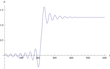
Figure 8: The evolutions of $\phi$ with respect to the time for the potential in the upper panel of Fig.7. The field, which is initially in a AdS minimum of its effective potential, goes through one single AdS cycle and finally lands at the dS minimum.

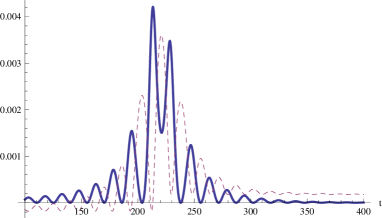
Figure 9: The solid line is the evolution of kinetic energy for the field in Fig.8, while the dashed line is the evolution of potential energy.

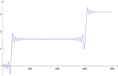
Figure 10: The evolution of $\phi$ with respect to the time for the potential in the lower panel of Fig.7. The field, which is initially in a AdS minimum of its effective potential, goes through two AdS cycles and finally lands at the dS minimum.

We plot the evolution of $\phi$ in Fig.8 for the potential in the upper panel of Fig.7, as well as the kinetic energy and the potential energy in Fig.9, and the evolution of $\phi$ in Fig.10 for the potential in the lower panel of Fig.7. During the contraction, the field $\phi$ oscillates around a AdS minimum of its potential, we have

$$\phi\simeq{C_{Mat}\over a^{3/2}}Sin\left({M_{\phi}(t_{B}-t)}\right),$$ (38)

where $C_{Mat}$ is the integral constant. In light of Eq.(38), this oscillation lasts for a period corresponds to $M_{\phi}\left(t_{Kin}-t_{*}\right)\gg\pi$, which equals to

$${M_{\phi}\over H_{*}}\gg 1,$$ (39)

since we generally have $|t_{*}|\gg|t_{Kin}|$. Thus noting $H_{*}\simeq\sqrt{|{\Lambda}_{*}|}/M_{P}$, in which ${\Lambda}_{*}$ is the depth of AdS minimum, we have

$$|{\Lambda}_{*}|\ll M_{\phi}^{2}M_{P}^{2}\,\,\lesssim V_{Bar},$$ (40)

where the width of the potential barrier is not larger than $M_{P}$ is required. The condition (40) is consistent with Eq.(25), which may be easily satisfied for any landscape, unless its AdS minimum are far deep.

We see that during the AdS bounce, the field will “fly” over the potential barrier, and finally land at other place of its effective potential. However, if where the field lands is a AdS minimum again, it will “fly” again until it finally lands at a dS minimum. Thus we may have a AdS cycles, during which the bubble universe goes through different AdS vacua.

References

- [1] A. Vilenkin, Phys. Rev. D27, 2848 (1983); A.D. Linde, Phys. Lett. B175, 395 (1986); P.J. Steinhardt, in “The Very Early Universe”, ed. by G.W. Gibbons, S.W. Hawking and S.T.C. Siklos (Cambridge University Press, 1983).
- [2] J. Garrige and A. Vilenkin, Phys. Rev. D57, 2230 (1998).
- [3] S. Dutta and T. Vachaspati, Phys. Rev. D71, 083507 (2005); S. Dutta, Phys. Rev. D73 (2006) 063524.
- [4] Y.S. Piao, Phys. Rev. D72, 103513 (2005); Phys. Lett. B659, 839 (2008); Phys. Rev. D79, 083512 (2009).
- [5] A. Aguirre and M. C. Johnson, Phys. Rev. D 73, 123529 (2006) [gr-qc/0512034].
- [6] W. Lee, B. -H. Lee, C. H. Lee and C. Park, Phys. Rev. D 74, 123520 (2006) [hep-th/0604064]; B. -H. Lee, C. H. Lee, W. Lee and C. Oh, arXiv:1311.4279 [hep-th].
- [7] V. A. Rubakov, Phys. Rev. D 88, 044015 (2013) [arXiv:1305.2614 [hep-th]].
- [8] Z. -G. Liu and Y. -S. Piao, Phys. Rev. D 88, 043520 (2013) [arXiv:1301.6833 [gr-qc]].
- [9] D. Hwang and D. Yeom, Class. Quant. Grav. 28, 155003 (2011) [arXiv:1010.3834 [gr-qc]].
- [10] J. Garriga and A. Vilenkin, arXiv:1210.7540 [hep-th].
- [11] Y. -S. Piao, Phys. Rev. D 70, 101302 (2004) [hep-th/0407258].
- [12] Y. -S. Piao, Phys. Lett. B 677, 1 (2009) [arXiv:0901.2644 [gr-qc]]; Y. -S. Piao, Phys. Lett. B 691, 225 (2010) [arXiv:1001.0631 [hep-th]].
- [13] M. C. Johnson and J. -L. Lehners, Phys. Rev. D 85, 103509 (2012) [arXiv:1112.3360 [hep-th]]; J. -L. Lehners, Phys. Rev. D 86, 043518 (2012) [arXiv:1206.1081 [hep-th]].
- [14] J. Garriga, A. Vilenkin and J. Zhang, JCAP 1311, 055 (2013) [arXiv:1309.2847 [hep-th]].
- [15] B. Gupt and P. Singh, arXiv:1309.2732 [hep-th].
- [16] V. Vanchurin and A. Vilenkin, Phys. Rev. D 74, 043520 (2006) [hep-th/0605015]; V. Vanchurin, Phys. Rev. D 75, 023524 (2007) [hep-th/0612215].
- [17] Y. -S. Piao, B. Feng and X. Zhang, Phys. Rev. D 69, 103520 (2004) [hep-th/0310206]; Y. -S. Piao, Phys. Rev. D 71, 087301 (2005) [astro-ph/0502343].
- [18] Z. G. Liu, Z. K. Guo and Y. S. Piao, Phys. Rev. D 88, 063539 (2013) [arXiv:1304.6527].
- [19] T. Biswas and A. Mazumdar, “Super-Inflation, Non-Singular Bounce, and Low Multipoles,” arXiv:1304.3648 [hep-th].
- [20] J. -Q. Xia, Y. -F. Cai, H. Li and X. Zhang, arXiv:1403.7623 [astro-ph.CO]; J. Liu, Y. -F. Cai and H. Li, J. Theor. Phys. 1, 1 (2012) [arXiv:1009.3372 [astro-ph.CO]].
- [21] T. Qiu, arXiv:1404.3060 [gr-qc].
- [22] J. Mielczarek, JCAP 0811, 011 (2008) [arXiv:0807.0712 [gr-qc]]; J. Mielczarek, M. Kamionka, A. Kurek and M. Szydlowski, JCAP 1007, 004 (2010) [arXiv:1005.0814 [gr-qc]].
- [23] R.C. Tolman, “Relativity, Thermodynamics and Cosmology”, (Oxford U. Press, Clarendon Press, 1934).
- [24] P.J. Steinhardt, N. Turok, Science 296, (2002) 1436; Phys. Rev. D65 126003 (2002).
- [25] J. D. Barrow and M. P. Dabrowski, Mon. Not. Roy. Astron. Soc. 275, 850 (1995).
- [26] N. Kanekar, V. Sahni and Y. Shtanov, Phys. Rev. D 63, 083520 (2001) [astro-ph/0101448].
- [27] V. Sahni and A. Toporensky, Phys. Rev. D 85, 123542 (2012) [arXiv:1203.0395 [gr-qc]].
- [28] Y. -S. Piao and Y. -Z. Zhang, Nucl. Phys. B 725, 265 (2005) [gr-qc/0407027].
- [29] H. -H. Xiong, Y. -F. Cai, T. Qiu, Y. -S. Piao and X. Zhang, Phys. Lett. B 666, 212 (2008) [arXiv:0805.0413 [astro-ph]]; Y. -F. Cai and E. N. Saridakis, J. Cosmol. 17, 7238 (2011) [arXiv:1108.6052 [gr-qc]].
- [30] T. Biswas, S. Alexander, Phys. Rev. D80, 043511 (2009); T. Biswas, A. Mazumdar, Phys. Rev. D80, 023519 (2009); W. Duhe and T. Biswas, arXiv:1306.6927 [astro-ph.CO].
- [31] K. Bamba, K. Yesmakhanova, K. Yerzhanov and R. Myrzakulov, Central Eur. J. Phys. 11, 397 (2013) [arXiv:1203.3401 [gr-qc]]; K. Bamba, U. Debnath, K. Yesmakhanova, P. Tsyba, G. Nugmanova and R. Myrzakulov, Entropy 14, 2351 (2012) [arXiv:1203.4226 [gr-qc]];
- [32] J. Zhang, Z. G. Liu and Y. S. Piao, Phys. Rev. D 82, 123505 (2010) [arXiv:1007.2498 [hep-th]].
- [33] P. W. Graham, B. Horn, S. Kachru, S. Rajendran and G. Torroba, arXiv:1109.0282 [hep-th].
- [34] J. -L. Lehners and P. J. Steinhardt, Phys. Rev. D 79, 063503 (2009) [arXiv:0812.3388 [hep-th]].
- [35] J. Garriga and A. Vilenkin, Phys. Rev. D 45, 3469 (1992).
- [36] J. Garriga, Phys. Rev. D 54, 4764 (1996) [gr-qc/9602025]; J. Garriga, X. Montes, M. Sasaki and T. Tanaka, Nucl. Phys. B 513, 343 (1998) [astro-ph/9706229]; J. Garcia-Bellido, J. Garriga and X. Montes, Phys. Rev. D 57, 4669 (1998) [hep-ph/9711214].
- [37] V.F. Mukhanov, JETP lett. 41, 493 (1985); Sov. Phys. JETP. 68, 1297 (1988).
- [38] H. Kodama, M. Sasaki, Prog. Theor. Phys. Suppl. 78 1 (1984).
- [39] Y. -F. Cai, T. Qiu, Y. -S. Piao, M. Li and X. Zhang, JHEP 0710, 071 (2007) [arXiv:0704.1090 [gr-qc]].
- [40] L. E. Allen and D. Wands, Phys. Rev. D 70, 063515 (2004) [astro-ph/0404441].
- [41] B. Xue, D. Garfinkle, F. Pretorius and P. J. Steinhardt, Phys. Rev. D 88 (2013) 083509 [arXiv:1308.3044 [gr-qc]].
- [42] J. Garriga, V.F. Mukhanov, Phys. Lett. B458, 219 (1999).
- [43] Z. -G. Liu and Y. -S. Piao, Phys. Rev. D 86, 083510 (2012) [arXiv:1201.1371 [gr-qc]].
- [44] L. Battarra, M. Koehn, J. -L. Lehners and B. A. Ovrut, arXiv:1404.5067 [hep-th].
- [45] D. Wands, Phys. Rev. D 60, 023507 (1999) [gr-qc/9809062].
- [46] F. Finelli and R. Brandenberger, Phys. Rev. D 65, 103522 (2002) [hep-th/0112249].
- [47] B. Freivogel, Class. Quant. Grav. 28, 204007 (2011) [arXiv:1105.0244 [hep-th]].
- [48] A. Vilenkin and J. Zhang, arXiv:1403.1599 [hep-th].
- [49] J. P. Conlon, JHEP 0605, 078 (2006) [hep-th/0602233].
- [50] R. Blumenhagen, X. Gao, T. Rahn and P. Shukla, JHEP 1206, 162 (2012) [arXiv:1205.2485 [hep-th]]. X. Gao and P. Shukla, arXiv:1307.1141 [hep-th].
- [51] T. Qiu, J. Evslin, Y. -F. Cai, M. Li and X. Zhang, JCAP 1110, 036 (2011) [arXiv:1108.0593 [hep-th]]; T. Qiu, X. Gao and E. N. Saridakis, Phys. Rev. D 88, 043525 (2013) [arXiv:1303.2372 [astro-ph.CO]].
- [52] D. A. Easson, I. Sawicki and A. Vikman, JCAP 1111, 021 (2011) [arXiv:1109.1047 [hep-th]].
- [53] Y. -F. Cai, D. A. Easson and R. Brandenberger, JCAP 1208, 020 (2012) [arXiv:1206.2382 [hep-th]].
- [54] M. Osipov and V. Rubakov, JCAP 1311, 031 (2013) [arXiv:1303.1221 [hep-th]].
- [55] M. Koehn, J. -L. Lehners and B. A. Ovrut, arXiv:1310.7577 [hep-th].
- [56] J. Khoury, B. A. Ovrut, P. J. Steinhardt and N. Turok, Phys. Rev. D 64, 123522 (2001) [hep-th/0103239]; E. I. Buchbinder, J. Khoury and B. A. Ovrut, Phys. Rev. D 76, 123503 (2007) [hep-th/0702154].
- [57] V. A. Rubakov, arXiv:1401.4024 [hep-th].
- [58] M. Gasperini and G. Veneziano, Astropart. Phys. 1, 317 (1993) [hep-th/9211021]; M. Gasperini and G. Veneziano, Phys. Rept. 373, 1 (2003) [hep-th/0207130].
- [59] T. Biswas, A. Mazumdar and W. Siegel, JCAP 0603, 009 (2006) [hep-th/0508194]; T. Biswas, E. Gerwick, T. Koivisto and A. Mazumdar, Phys. Rev. Lett. 108, 031101 (2012) [arXiv:1110.5249 [gr-qc]]; T. Biswas, A. S. Koshelev, A. Mazumdar and S. Y. .Vernov, JCAP 1208, 024 (2012) [arXiv:1206.6374 [astro-ph.CO]].
- [60] Y. -S. Piao, S. Tsujikawa and X. Zhang, Class. Quant. Grav. 21, 4455 (2004) [hep-th/0312139].
- [61] G. Calcagni, JHEP 1003, 120 (2010) [arXiv:1001.0571 [hep-th]]; G. Calcagni, JCAP12(2013)041 [arXiv:1307.6382 [hep-th]].
- [62] K. Bamba, A. N. Makarenko, A. N. Myagky, S. ’i. Nojiri and S. D. Odintsov, arXiv:1309.3748 [hep-th]; K. Bamba, A. N. Makarenko, A. N. Myagky and S. D. Odintsov, arXiv:1403.3242 [hep-th].
- [63] M. Novello, S.E.P. Bergliaffa, Phys. Rept. 463, 127 (2008).
- [64] J. -L. Lehners, Class. Quant. Grav. 28, 204004 (2011) [arXiv:1106.0172 [hep-th]].
- [65] Y. Shtanov and V. Sahni, Phys. Lett. B 557, 1 (2003) [gr-qc/0208047].
- [66] A. Ashtekar and P. Singh, Class. Quant. Grav. 28, 213001 (2011) [arXiv:1108.0893 [gr-qc]].