Quantum discord for general X and CS states: A piecewise-analytic-numerical formula

M. A. Yurischev yur@itp.ac.ru Institute of Problems of Chemical Physics of the Russian Academy of Sciences, 142432 Chernogolovka, Moscow Region, Russia
Abstract

Quantum discord is a function of density-matrix elements (and through them, e. g., of temperature, applied fields, time, and so forth). The domain of such a function in the case of two-qubit system with X or centrosymmetric (CS) density matrix can consist at most of three subdomains: two ones, where the quantum discord is expressed in closed analytical forms ($Q_{0}$ and $Q_{\pi/2}$), and an intermediate subdomain in which for determining the quantum discord $Q_{\theta}$ it is required to solve numerically a one-dimensional minimization problem to find the optimal measurement angle $\theta\in(0,\pi/2)$. Exact equations for determining the boundaries between these subdomains are obtained and solved for a number of models. The $Q_{\theta}$ subdomains are discovered in the anisotropic spin dimers in external field. On the other hand, coinciding boundaries and therefore sudden transitions between optimal measurement angles $\theta=\pi/2$ and $\theta=0$ are observed in dynamics of spin currying particles in closed nanopore and also in phase flip channels. In latter cases the solutions are entirely analytical.

pacs:
03.65.Ud, 03.67.-a, 75.10.Jm

I Introduction

Quantum correlation theory is one of the most rapid developed direction in modern physics. This theory is important for the new technologies related to an utilization of quantum information processing.

Earlier, only the quantum entanglement was attributed to quantum correlations AFOV08 ; HHHH09 . The quantum entanglement exists in non-separable states of a system. However in the last years one came to a conclusion that the quantum correlations can be present in mixed separable states, i. e., when the quantum entanglement is absent. As a measure of total purely quantum correlations one takes now the quantum discord CMS11 ; MBCPV12 ; AFY14 . In the ground of discord conception lies the idea of measurements performed on the system or its parts and extracting with their help a maximum amount of information.

Due to necessary to solve the optimization problem, the evaluation of quantum correlations, especially discord, is extremely hard. If for the two-qubit systems the quantum entanglement has been obtained for the arbitrary density matrices W98 , the analytical formulas for the quantum discord were proposed only for X or CS states Luo08 ; ARA10 ; FWBAC10 ; LWF11 ; DWZ11 ; Y13 . In an X matrix, nonzero entries may belong only to the main diagonal and anti-diagonal. The $n\times n$ CS matrix is defined by the relations for its elements: $a_{i,j}=a_{n-i+1,n-j+1}$. Any CS matrix of fourth order takes the X form under the double Hadamard transformation $H\otimes H$ ($H$ is the ordinary Hadamard matrix) Y13 . This transformation belongs to the class of local unitary transformations and therefore the quantum correlations do not change their values.

However, it was latter found LMXW11 ; CZYYO11 ; H13 that the formulas for X states ARA10 ; FWBAC10 ; LWF11 are not always correct. The reason is that the authors ARA10 ; FWBAC10 ; LWF11 believed (and this was their error) that the optimal measurements are achieved only in the limiting points, i. e., at the angles $\theta=0$ or $\pi/2$ (see below). But on the explicit examples LMXW11 ; CZYYO11 ; H13 of X density matrices it was proved that that the optimal measurements can take places at the intermediate angles in the interval $(0,\pi/2)$. Unfortunately, these examples with the density matrices do not clarify the physical situation.

In the present paper we use the language of Hamiltonians. We show that the domain of intermediate optimal angles can arise in the vicinity of transition from the domain with optimal measurement angle $\theta=\pi/2$ to the domain with optimal angle $\theta=0$ (or vice versa). We obtain the equations for the boundaries between these domains and investigate their solutions for some models.

In the following sections we establish an isomorphism between the X density matrices and Gibbs ones with XYZ Hamiltonians, prove the existence of intermediate domains (with the optimal anglers $\theta\not=0,\pi/2$), derive the equations for boundaries between different domains, and, finally, apply the developed approach to a gas of spin-carrying particles in closed nanopore and to a phase flip channel.

II X density matrices and XYZ spin dimers

In the most general form, the X density matrix of two-qubit system is given as

$$\rho=\left(\begin{array}[]{cccc}a&0&0&u_{1}+iu_{2}\\ 0&b&v_{1}+iv_{2}&0\\ 0&v_{1}-iv_{2}&c&0\\ u_{1}-iu_{2}&0&0&d\end{array}\right),$$ (1)

where $a+b+c+d=1$. This matrix contains seven real parameters which must satisfy the inequalities

$$a,b,c,d\geq 0,\quad ad\geq u_{1}^{2}+u_{2}^{2},\quad bc\geq v_{1}^{2}+v_{2}^{2}.$$ (2)

Decomposition of the matrix (1) on the Pauli matrices $\sigma_{\alpha}$ ($\alpha=x,y,z$) leads to its Bloch form

$\displaystyle\rho$ $\displaystyle=$ $\displaystyle{1\over 4}\{1-[1-2(a+b)]\sigma_{z}\otimes 1-[1-2(a+c)]1\otimes\sigma_{z}+2(u_{1}+v_{1})\sigma_{x}\otimes\sigma_{x}$ (3)
$\displaystyle+$ $\displaystyle 2(v_{1}-u_{1})\sigma_{y}\otimes\sigma_{y}+[1-2(b+c)]\sigma_{z}\otimes\sigma_{z}-2(u_{2}-v_{2})\sigma_{x}\otimes\sigma_{y}$
$\displaystyle-$ $\displaystyle 2(u_{2}+v_{2})\sigma_{y}\otimes\sigma_{x}\}$

The expansion coefficients are the unary and binary correlation functions and therefore seven parameters of density matrix are expressed through the seven different correlators.

To clarify the reasons for appearance of intermediate optimal measurements, consider the spin-1/2 dimers in thermal equilibrium state. In accord with Eq. (3) we take the Hamiltonian in the form

$${\cal H}=-{1\over 2}(J_{x}\sigma_{1}^{x}\sigma_{2}^{x}+J_{y}\sigma_{1}^{y}\sigma_{2}^{y}+J_{z}\sigma_{1}^{z}\sigma_{2}^{z}+B_{1}\sigma_{1}^{z}+B_{2}\sigma_{2}^{z})+J_{xy}\sigma_{1}^{x}\sigma_{2}^{y}+J_{yx}\sigma_{1}^{y}\sigma_{2}^{x},$$ (4)

where $\sigma_{i}^{\alpha}$ is the $\alpha$-th Pauli matrix in the $i$-th site, and $J_{x},J_{y},J_{z},B_{1},B_{2},J_{xy}$, and $J_{yx}$ are seven arbitrary real parameters. The corresponding Gibbs density matrix

$$\rho={1\over Z}e^{-{\cal H}/T}$$ (5)

($T$ is the temperature in energy units and $Z$ is the partition function) has the seven-parameter X form. This circumstance allows to come from the formal density-matrix language to the physically clear picture of interactions in the system.

The quantum entanglement and quantum discord are invariant under the local unitary transformations AFOV08 ; HHHH09 ; CMS11 ; MBCPV12 ; AFY14 . Thanks to this property, one can with the help of transformation

$$U=e^{-i\varphi_{1}\sigma_{z}/2}\otimes e^{-i\varphi_{2}\sigma_{z}/2}$$ (6)

reduce the seven-parameters density matrix (1) to the real five-parameters X form H13 ; CRC10 . This provides with the angles

$$\varphi_{1,2}={1\over 2}(\arctan{u_{2}\over u_{1}}\pm\arctan{v_{2}\over v_{1}}).$$ (7)

After this, the density matrix (1) takes the form

$$\rho=\left(\begin{array}[]{cccc}a&0&0&u\\ 0&b&v&0\\ 0&v&c&0\\ u&0&0&d\end{array}\right),$$ (8)

where

$$u=u_{1}\cos(\arctan{u_{2}\over u_{1}})+u_{2}\sin(\arctan{u_{2}\over u_{1}}),$$ (9)
$$v=v_{1}\cos(\arctan{v_{2}\over v_{1}})+v_{2}\sin(\arctan{v_{2}\over v_{1}}).$$ (10)

Moreover, with the help of local rotations again around the $z$ axis, it is not difficult to obtain also the non-negative off-diagonal elements of the X matrix (8). Indeed, the local unitary transformation

$$U_{1}=e^{-i{\pi\over 4}\sigma_{z}}\otimes e^{i{\pi\over 4}\sigma_{z}}=\left(\begin{array}[]{cccc}i&&&\\ &1&&\\ &&1&\\ &&&-i\end{array}\right),$$ (11)

leads to a change of sign for $u$:

$$U_{1}\rho U_{1}^{+}=\left(\begin{array}[]{rrrr}a&0&0&-u\\ 0&b&v&0\\ 0&v&c&0\\ -u&0&0&d\end{array}\right).$$ (12)

Similarly, the local transformation

$$U_{2}=e^{i{\pi\over 4}\sigma_{z}}\otimes e^{-i{\pi\over 4}\sigma_{z}}=\left(\begin{array}[]{cccc}1&&&\\ &i&&\\ &&-i&\\ &&&1\end{array}\right),$$ (13)

selectively acts on the sign of $v$:

$$U_{2}\rho U_{2}^{+}=\left(\begin{array}[]{rrrr}a&0&0&u\\ 0&b&-v&0\\ 0&-v&c&0\\ u&0&0&d\end{array}\right).$$ (14)

Thus, after transformation of an X matrix to the real form we may simply enclose the off-diagonal elements in the modul symbols:

$$\rho=\left(\begin{array}[]{cccc}a&0&0&|u|\\ 0&b&|v|&0\\ 0&|v|&c&0\\ |u|&0&0&d\end{array}\right).$$ (15)

This operation does not influence on the value of quantum correlations in a system.

It is not difficult to understand that all peculiarities of discord behavior in the states with seven-parameters density matrix (1) can be described by the thermal density matrix of XYZ dimer in inhomogeneous fields $B_{1}$ and $B_{2}$ without crossing terms $J_{xy}$ and $J_{yx}$,

$${\cal H}=-{1\over 2}(J_{x}\sigma_{1}^{x}\sigma_{2}^{x}+J_{y}\sigma_{1}^{y}\sigma_{2}^{y}+J_{z}\sigma_{1}^{z}\sigma_{2}^{z}+B_{1}\sigma_{1}^{z}+B_{2}\sigma_{2}^{z}).$$ (16)

This model contains five independent parameters $J_{x},J_{y},J_{z},B_{1}$, and $B_{2}$.

III Three alternatives for the quantum discord

As mentioned above, the measurement operations lie in the ground of discord notion. Following the founders of discord conception OZ01 ; Z03 and their adherents Luo08 ; ARA10 ; FWBAC10 ; LWF11 ; DWZ11 proposed the formulas for calculation of quantum discord in two-qubit systems, we will consider here only the projective measurements rem1 . For the X state (3) and XYZ dimer (16), $z$-direction is, obviously, peculiar. Therefore, the measurements can be reduced to projections which are characterized by the polar ($\theta$) and azimuthal ($\phi$) angles relative to the $z$-axis. It is important that in the case of real X density matrix with an additional condition $uv\geq 0$ the optimal measurements are achieved by $\cos 2\phi=1$ H13 ; CRC10 .

Let the spins 1 and 2 of a dimer be the subsystems $A$ and $B$, respectively. Denote the density matrix of total system as $\rho_{AB}\ (=\rho)$, and for the reduced density matrices we will use the notations $\rho_{A}$ and $\rho_{B}$:

$$\rho_{A}={\rm Tr}_{B}\rho_{AB}=\left(\begin{array}[]{cc}a+b&0\\ 0&c+d\end{array}\right),$$ (17)
$$\rho_{B}={\rm Tr}_{A}\rho_{AB}=\left(\begin{array}[]{cc}a+c&0\\ 0&b+d\end{array}\right).$$ (18)

Quantum discord in general depends on which subsystem ($A$ or $B$) the measurements are performed. Let, for definiteness, the measured subsystem be $B$. Then the quantum discord is given as

$$Q=S(\rho_{B})-S(\rho_{AB})+\min_{\theta}S_{cond}(\theta).$$ (19)

Here $S(\rho)=-{\rm Tr}\rho\ln\rho$ is the von Neumann entropy (in nats) for corresponding state $\rho$:

$$S(\rho_{B})=-(a+c)\ln(a+c)-(b+d)\ln(b+d),$$ (20)
$\displaystyle S(\rho_{AB})\equiv S$
$\displaystyle=-{a+d+\sqrt{(a-d)^{2}+4u^{2}}\over 2}\ln{a+d+\sqrt{(a-d)^{2}+4u^{2}}\over 2}$
$\displaystyle-{a+d-\sqrt{(a-d)^{2}+4u^{2}}\over 2}\ln{a+d-\sqrt{(a-d)^{2}+4u^{2}}\over 2}$
$\displaystyle-{b+c+\sqrt{(b-c)^{2}+4v^{2}}\over 2}\ln{b+c+\sqrt{(b-c)^{2}+4v^{2}}\over 2}$
$\displaystyle-{b+c-\sqrt{(b-c)^{2}+4v^{2}}\over 2}\ln{b+c-\sqrt{(b-c)^{2}+4v^{2}}\over 2}.$ (21)

Taking into account that $\cos 2\phi=1$, the quantum conditional entropy of subsystem $A$ is given as H13

$$S_{cond}(\theta)=\Lambda_{1}\ln\Lambda_{1}+\Lambda_{2}\ln\Lambda_{2}-\sum_{i=1}^{4}\lambda_{i}\ln\lambda_{i},$$ (22)

where

$$\Lambda_{1,2}={1\over 2}[1\pm(a-b+c-d)\cos\theta],$$ (23)
$\displaystyle\lambda_{1,2}$ $\displaystyle=$ $\displaystyle{1\over 4}[\![1+(a-b+c-d)\cos\theta$ (24)
$\displaystyle\pm$ $\displaystyle\{[a+b-c-d+(a-b-c+d)\cos\theta]^{2}+4(|u|+|v|)^{2}\sin^{2}\theta\}^{1/2}]\!],$
$\displaystyle\lambda_{3,4}$ $\displaystyle=$ $\displaystyle{1\over 4}[\![1-(a-b+c-d)\cos\theta$ (25)
$\displaystyle\pm$ $\displaystyle\{[a+b-c-d-(a-b-c+d)\cos\theta]^{2}+4(|u|+|v|)^{2}\sin^{2}\theta\}^{1/2}]\!].$

The conditional entropy $S_{cond}(\theta)$ is a continuous and differentiable function of its argument $\theta$.

Expressions (20)-(25) allows to define the measurement-dependent discord as

$$Q(\theta)=S(\rho_{B})-S(\rho_{AB})+S_{cond}(\theta),$$ (26)

where $\theta\in[0,\pi/2]$. The absolute minimum of this discord can be, obviously, either on the bounds ($\theta=0,\pi/2$) or at the intermediate point $\theta\in(0,\pi/2)$. As a result, there is a choice from three corresponding possibilities for the quantum discord

$$Q=\min\{Q_{0},Q_{\theta},Q_{\pi\over 2}\}.$$ (27)

This equation generalizes the earlier proposed one for the quantum discord Luo08 ; ARA10 ; FWBAC10 ; LWF11 ; DWZ11

$$\tilde{Q}=\min\{Q_{0},Q_{\pi\over 2}\},$$ (28)

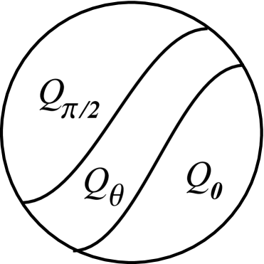
i. e., the optimal observable can be either $\sigma_{x}$ or $\sigma_{z}$. In Fig. 1 we schematically represent the parameter domain of a system with three possible subdomains for the discord.

From the expressions (20)-(26), we have for the discord branch $Q_{0}\equiv Q(0)$:

$$Q_{0}=-S-a\ln a-b\ln b-c\ln c-d\ln d.$$ (29)

By $\theta=\pi/2$ we obtain

$\displaystyle Q_{\pi\over 2}=-S-\ln 2-(a+c)\ln(a+c)-(b+d)\ln(b+d)$
$\displaystyle-{1+\sqrt{(a+b-c-d)^{2}+4(|u|+|v|)^{2}}\over 2}\ln{1+\sqrt{(a+b-c-d)^{2}+4(|u|+|v|)^{2}}\over 4}$
$\displaystyle-{1-\sqrt{(a+b-c-d)^{2}+4(|u|+|v|)^{2}}\over 2}\ln{1-\sqrt{(a+b-c-d)^{2}+4(|u|+|v|)^{2}}\over 4}.$ (30)

Thus, the branches $Q_{0}$ and $Q_{\pi/2}$ are expressed analytically, and the branch $Q_{\theta}=\min\nolimits_{\theta\in(0,\pi/2)}Q(\theta)$, if the intermediate minimum exists, should be found from the numerical solution of one-dimensional minimization problem or from the transcendental equation

$$S^{\prime}_{cond}(\theta)=0,$$ (31)

where the derivative of conditional entropy with respect to $\theta$ is equal to

$$S^{\prime}_{cond}(\theta)=\Lambda^{\prime}_{1}(1+\ln\Lambda_{1})+\Lambda^{\prime}_{2}(1+\ln\Lambda_{2})-\sum_{i=1}^{4}\lambda^{\prime}_{i}(1+\ln\lambda_{i})$$ (32)

with

$$\Lambda^{\prime}_{1,2}=\mp{1\over 2}(a-b+c-d)\sin\theta,$$ (33)
$\displaystyle\lambda^{\prime}_{1,2}={1\over 4}\bigg{[}-(a-b+c-d)\sin\theta$
$\displaystyle\pm\frac{[a+b-c-d+(a-b-c+d)\cos\theta][-(a-b-c+d)\sin\theta]+2(|u|+|v|)^{2}\sin 2\theta}{\sqrt{[a+b-c-d+(a-b-c+d)\cos\theta]^{2}+4(|u|+|v|)^{2}\sin^{2}\theta}}\bigg{]},\quad$ (34)
$\displaystyle\lambda^{\prime}_{3,4}={1\over 4}\bigg{[}(a-b+c-d)\sin\theta$
$\displaystyle\pm\frac{[a+b-c-d-(a-b-c+d)\cos\theta](a-b-c+d)\sin\theta+2(|u|+|v|)^{2}\sin 2\theta}{\sqrt{[a+b-c-d-(a-b-c+d)\cos\theta]^{2}+4(|u|+|v|)^{2}\sin^{2}\theta}}\bigg{]}.$ (35)

All three possible variants for the quantum discord ($Q_{0}$, $Q_{\pi/2}$, and $Q_{\theta}$) can really exist in physical systems. In the case when $a=b$ and $b=c$ (for example, the thermal discord for XYZ dimers in absence of external field) the conditional entropy minimum is achieved always at the bound points Luo08 . The authors ARA10 ; FWBAC10 ; LWF11 ; DWZ11 have then extended the limiting possibilities to the more general X states. However, this is wrong; the minimum can take place at inner points.

Indeed, following the authors LMXW11 , consider the state

$$\rho=\left(\begin{array}[]{cccc}0.0783&0&0&0\\ 0&0.125&0.100&0\\ 0&0.100&0.125&0\\ 0&0&0&0.6717\end{array}\right).$$ (36)

Using Eqs. (22)-(25) we computed the function $S_{cond}(\theta)$ for this state. Its behavior is shown in Fig. 2. It is clear seen that the conditional entropy minimum is situated in the intermediate region, namely at the angle $\theta=0.4883\approx 28^{\circ}$. The quantum discord value is on $6.7\times 10^{-6}$ less than the value with $\theta=0$.

In the paper H13 , other examples are given. In particular, for the quantum state

$$\rho=\left(\begin{array}[]{cccc}0.021\,726&0&0&0.128\,057\\ 0&0.010\,288&0&0\\ 0&0&0.010\,288&0\\ 0.128\,057&0&0&0.957\,698\end{array}\right)$$ (37)

the error for discord is here grater and equals $5.7\times 10^{-4}$. The behavior of $S_{cond}(\theta)$ for this state is depicted in Fig. 3.

These examples clearly show that the optimal measurement angles can really be in the intermediate region $(0,\pi/2)$, i. e., the optimal observables for quantum discord can be not only the $\sigma_{x}$ or $\sigma_{z}$, but also their superposition.

For the real X state with constraint $|u+v|\geq|u-v|$, the authors CZYYO11 have proven a theorem which guarantees that the optimal observable is $\sigma_{z}$ if

$$(|u|+|v|)^{2}\leq(a-b)(d-c)$$ (38)

and $\sigma_{x}$ if

$$|\sqrt{ad}-\sqrt{bc}\leq|u|+|v|.$$ (39)

The theorem claims nothing for the region between these inequalities. But in the case

$$ac=bd$$ (40)

the inequalities (38) and (39) lead to absence of any intermediate region PKF13 . In particular, this is valid for the Bell-diagonal states because for them $a=d$ and $b=c$.

IV Equations for the exact boundaries

Start with a heuristic example. Consider the XXZ dimer in an uniform external field. Its Hamiltonian is written as

$${\cal H}=-{1\over 2}J(\sigma_{1}^{x}\sigma_{2}^{x}+\sigma_{1}^{y}\sigma_{2}^{y}+\Delta\sigma_{1}^{z}\sigma_{2}^{z})-{1\over 2}B(\sigma_{1}^{z}+\sigma_{2}^{z}),$$ (41)

where $\Delta=J_{z}/J$ is the coupling anisotropy. The Gibbs density matrix is equal to

$$\rho=\left(\begin{array}[]{cccc}a&&&\\ &b&v&\\ &v&b&\\ &&&d\end{array}\right),$$ (42)

where

$$a={1\over Z}e^{(J_{z}/2+B)/T},\quad b={1\over Z}e^{-J_{z}/2T}\cosh{J\over T},\quad d={1\over Z}e^{(J_{z}/2-B)/T},\quad v={1\over Z}e^{-J_{z}/2T}\sinh{J\over T},$$ (43)

and the partition function

$$Z=2(e^{J_{z}/2T}\cosh{B\over T}+e^{-J_{z}/2T}\cosh{J\over T}).$$ (44)

These expressions allow to determine the parameters of the Hamiltonian (41):

$$J={T\over 2}\ln\frac{1+v/b}{1-v/b},\quad J_{z}={T\over 2}\ln\frac{ad}{b^{2}-v^{2}},\quad B={T\over 2}\ln{a\over d}.$$ (45)

Returning to the examples from the previous section we find that the state (36) is realized for the dimer (41) with the parameters $J=1$, $J_{z}=1.017\approx 1.02$, and $B=-0.98$ at the temperature $T=1.1$. These values are quite reasonable.

Will now for each choice of interaction constants $J$ and $J_{z}$ find, on the plane temperature-field, the lines which defined by the condition

$$Q_{0}(T,B)=Q_{\pi\over 2}(T,B).$$ (46)

After this we will study the changes of curves $S_{cond}(\theta)$ in the neighborhood of those lines.

Using Eqs. (III), (29), (III), (43), and (44) we have numerically solved the transcendental equation (46) by $J=1$ and different values of $\Delta=J_{z}/J$. The results are shown in Fig. 4 by dashed lines.

Consider in detail, for example, the case $\Delta=1.02$ (the 5th line in Fig. 4). Let the external field is held fixed and equal to $B=1$. Then the equality $Q_{0}=Q_{\pi/2}$ is satisfied at the temperature $T_{\times}=0.81296$. Study now the behavior of $S_{cond}(\theta)$ when the temperature varies. If $T=0.76$, the minimum of $S_{cond}(\theta)$ is at $\theta=\pi/2$ (see Fig. 5). The angle $\theta=\pi/2$ is optimal for all lower temperatures. When the temperature increases, it is appeared the minimum on the curve $S_{cond}(\theta)$ inside the interval between 0 and $\pi/2$. The minimum is clear seen by $T=0.79$ (Fig. 6). Near the point $T_{\times}=0.81296$ the minimum achieves the maximal depth (see Fig. 7). With further increasing the temperature the minimum moves to the bound $\theta=0$ (Fig. 8) and then it disappears at all (Fig. 9). Optimal measurements undergo to the angle $\theta=0$.

Argue now that both lower and upper boundaries of the interval within which the optimal angles lie between 0 and $\pi/2$ are exact, i. e., the intermediate minimum of $S_{cond}(\theta)$ suddenly appears and suddenly disappears. First of all, we note that the derivatives of function $S_{cond}(\theta)$ at $\theta=0$ and $\pi/2$ equal zero in general case: $S^{\prime}_{cond}(0)=S^{\prime}_{cond}(\pi/2)=0$. This is easy to check by direct calculations using Eqs. (32)-(III). Turn now again to the Figs. 5-9. By every fixed value of external field $B$ and for each value of temperature $T$ one can at any moment to say either exist the inside minimum or not. For instance, when $T=0.76$ ($B=1$) the function $S_{cond}(\theta)$ is concave at the point $\theta=\pi/2$ and therefore its second derivative $S^{\prime\prime}_{cond}(\pi/2)<0$. But when $T=0.79$ the conditional entropy has a local maximum at the same bound point $\theta=\pi/2$ and therefore $S^{\prime\prime}_{cond}(\pi/2)>0$. Hence, the bifurcation point (doubling the extremum) is determined by the condition

$$S^{\prime\prime}_{cond}(\pi/2)=0.$$ (47)

Similarly for the other bound point $\theta=0$:

$$S^{\prime\prime}_{cond}(0)=0.$$ (48)

Using Eqs. (22)-(25) we obtain the second derivatives at limiting points:

$\displaystyle S^{\prime\prime}_{cond}(0)$ $\displaystyle=$ $\displaystyle{1\over 4}(a-b+c-d)\biggl{(}2\ln\frac{b+d}{a+c}+\ln{ac\over bd}\biggr{)}$ (49)
$\displaystyle+{1\over 4}(a-b-c+d)\ln{ad\over bc}-{1\over 2}(|u|+|v|)^{2}\biggl{(}{1\over a-c}\ln{a\over c}+{1\over b-d}\ln{b\over d}\biggr{)}$

and

$\displaystyle S^{\prime\prime}_{cond}(\pi/2)$ $\displaystyle=$ $\displaystyle(a-b+c-d)^{2}$ (50)
$\displaystyle-{1\over 2(1+r)}\bigl{[}a-b+c-d+{1\over r}(a+b-c-d)(a-b-c+d)\bigl{]}^{2}$
$\displaystyle-{1\over 2(1-r)}\bigl{[}a-b+c-d-{1\over r}(a+b-c-d)(a-b-c+d)\bigl{]}^{2}$
$\displaystyle+{1\over 2r}\{(a-b-c+d)^{2}[1-{1\over r^{2}}(a+b-c-d)^{2}]-4(|u|+|v|)^{2}\}\ln\frac{1-r}{1+r},$

where

$$r=[(a+b-c-d)^{2}+4(|u|+|v|)^{2}]^{1/2}.$$ (51)

The relations (48)-(51) are the boundary equations for the crossover subdomain $Q_{\theta}$.

If the solutions of Eqs. (47) and (48) are the same then the intermediate domain $Q_{\theta}$ is absent and the quantum discord is given by analytical expressions. On the other hand, instead roughly conditions (38) and (39), the inequalities $S^{\prime\prime}_{cond}(0)\leq 0$ and $S^{\prime\prime}_{cond}(\pi/2)\leq 0$ define now the whole subdomains $Q_{0}$ and $Q_{\pi/2}$ respectively.

Numerical solution of Eqs. (48)-(51) for the XXZ dimer shows that the boundaries are the lines going approximately parallel to the dashed lines (see the lines 5a and 5b in Fig. 4). As a result, it is arisen a domain within which the optimal angles should be found numerically. Out of this domain we have analytical expressions for the quantum discord. To not clutter up the Fig. 4, we show a part of intermediate domain only for the case $\Delta=1.02$. By $B=1$, the temperature of $\pi/2$-boundary equals $T_{\pi/2}=0.76106$ and for the 0-boundary $T_{0}=0.85361$. The middle of this interval equals 0.80734 which is near the point $T_{\times}=0.81296$. The relative width of this interval is 11.5%.

Using the example of XXZ dimer with parameters $J=1$, $J_{z}=1.02$, and $B=1$ consider the thermal discord behavior by a transition from the domain $Q_{\pi/2}$ into $Q_{0}$ one. For this case, the functions $Q_{0}$ and $Q_{\pi/2}$ versus the temperature are shown in Fig. 10. One can see that down to crossing point $T_{\times}=0.81296$ the discord (${\tilde{Q}}$) as a minimal value would be according Refs. ARA10 -LWF11 equals $Q_{\pi/2}$, and above the intersection point $T_{\times}$ equals $Q_{0}$. If this would be valid, the discord ${\tilde{Q}}=\min\{Q_{0},Q_{\pi/2}\}$ at the intersection point $T_{\times}$ would be not differentiable. However, in reality the function is smooth. This follows from the numerical solution of the task in the intermediate domain. The results are shown in Fig. 11. It is clearly seen that the smoothness occurs. By this, the correction $\Delta Q={\tilde{Q}}-Q$ has a small value. The behavior of $\Delta Q$ is shown in Fig. 12. The curve has a cusp-like form. The largest deviation $\Delta Q=3.1\times 10^{-5}$ is about 0.03%.

A two-parameter family of X states

$$\rho=\left(\begin{array}[]{cccc}\epsilon/2&0&0&\epsilon/2\\ 0&(1-\epsilon)m&0&0\\ 0&0&(1-\epsilon)(1-m)&0\\ \epsilon/2&0&0&\epsilon/2\end{array}\right),$$ (52)

was considered in Ref. CZYYO11 . Using Eqs. (47)-(51) we calculated the lower and upper boundaries for the state (52). The results are presented in Fig. 13. Note that the sufficient conditions (38) and (39) for the $Q_{0}$ and $Q_{\pi/2}$ domains give CZYYO11

$$\epsilon\leq\frac{2m(1-m)}{1+2m(1-m)}$$ (53)

and

$$\epsilon\geq\frac{\sqrt{m(1-m)}}{1+\sqrt{m(1-m)}}$$ (54)

respectively. Unfortunately, these boundaries rough too and lie far out the region of Fig. 13.

Notice, the boundaries may coincide between themselves. Moreover, by coinciding boundaries, the cases can take places when there are no smoothing for the quantum discord. Such examples we discuss in the following sections.

V CS density matrices. Gas in nanopore

As has been shown in Ref. FKY12 , the reduced density matrix for any pair of nuclear spins in a closed nanopore filled with a gas of spin-carrying molecules has the CS form

$$\rho=\left(\begin{array}[]{cccc}{1\over 4}&{1\over 2}p-iu&{1\over 2}p-iu&q-r\\ {1\over 2}p+iu&{1\over 4}&q+r&{1\over 2}p+iu\\ {1\over 2}p+iu&q+r&{1\over 4}&{1\over 2}p+iu\\ q-r&{1\over 2}p-iu&{1\over 2}p-iu&{1\over 4}\end{array}\right),$$ (55)

where

$\displaystyle p={1\over 2}\tanh{\beta\over 2}\cos^{N-1}(at),$
$\displaystyle q={1\over 8}\tanh^{2}{\beta\over 2}[1+\cos^{N-2}(2at)],$
$\displaystyle r={1\over 8}\tanh^{2}{\beta\over 2}[1-\cos^{N-2}(2at)],$ (56)
$\displaystyle u={1\over 4}\tanh{\beta\over 2}\cos^{N-2}(at)\sin(at).$

(One should not confuse the defined here quantities $u$ and $r$ with the same denoted quantities from the previous sections.) In relations (V), $N$ is the number of particles confined in a nanopore, $\beta$ is the inverse dimensionless temperature, and $\alpha t$ is the dimensionless time.

After transformation to the real X form, the density matrix (55) takes the form

$$\rho=\left(\begin{array}[]{cccc}{1\over 4}+p+q&0&0&2u\sin 2\varphi-r\cos 2\varphi\\ 0&{1\over 4}-q&r&0\\ 0&r&{1\over 4}-q&0\\ 2u\sin 2\varphi-r\cos 2\varphi&0&0&{1\over 4}-p+q\end{array}\right),$$ (57)

where

$$\varphi=-{1\over 2}\arctan(2u/r).$$ (58)

Using the analytical formulas FWBAC10 which are valid in a supposition that the quantum conditional entropy has minimums only at the bound points, the author Y13 found the quantum discord for particles in nanopore. Here we prove that in the case of nanopore the intermediate optimal angle domain does not exist and therefore the results Y13 are correct.

Applying the approach discussed above we study the behavior of functions $Q_{0}(\alpha t)$ and $Q_{\pi/2}(\alpha t)$ by fixed values of $N$ and $\beta$. The behavior of these quantities (in bits!) by $N=10$ and $\beta=1$ is shown in Fig. 14. Both functions are periodic with the period equals $\pi$. In the interval $0<\alpha t<\pi$, the curves are crossed at points $\alpha t_{1}=0.98486$ and $\alpha t_{2}=2.15673$ (see Fig. 14). A solution of boundary equations (48)-(51) shows that in this case both boundaries coincide between themselves. Thus, for the discussed system there are not domains where the conditional entropy has the intermediate minimum. Changes of the function $S_{cond}(\theta)$ in the vicinity of point $\alpha t_{1}$ is shown in Fig. 15. When $t<t_{1}$, the conditional entropy has a minimum at $\theta=\pi/2$ (curves 1 and 2 in Fig. 15). At $t=t_{1}$, the function $S_{cond}(\theta)$ becomes a straight line. This is the point of indifference to a choice of measurement angle: $\forall~{}\theta\in[0,\pi/2]$. With further increasing $\alpha t$, the minimum of $S_{cond}(\theta)$ lies at the second bound $\theta=0$. At the another crossing point $\alpha t_{2}$ the quantum discord goes, vice versa, from the branch $Q_{0}$ to $Q_{\pi/2}$, and so on. Thus, the quantum discord $Q(\alpha t)=\min\{Q_{0},Q_{\pi/2}\}$ is given here in a closed analytical form. Note that this function is smooth at the crossing points.

For odd $N$, the solution is another. In this case there are no crossing points of curves $Q_{0}(\alpha t)$ and $Q_{\pi/2}(\alpha t)$ and the quantum discord at any time is defined by the branch $Q_{\pi/2}(\alpha t)$.

So, the quantum discord for nanopore is an analytical or piecewise analytical function.

VI Phase flip channel

The authors LWF11 have considered the dynamics of quantum discord under decoherence in a phase flip channel. The problem is to calculate the quantum discord for the X matrix

$\displaystyle\varepsilon$ $\displaystyle=$ $\displaystyle{1\over 4}[1+r\sigma_{z}\otimes 1+s1\otimes\sigma_{z}+(1-p)^{2}c_{1}\sigma_{x}\otimes\sigma_{x}$ (59)
$\displaystyle+$ $\displaystyle(1-p)^{2}c_{2}\sigma_{y}\otimes\sigma_{y}+c_{3}\sigma_{z}\otimes\sigma_{z}],$

where $p=1-\exp(-\gamma t)$, $t$ is the time, and $\gamma$ is the phase damping rate. The authors LWF11 restricted themselves to the case where

$$c_{2}=-c_{3}c_{1},\qquad s=c_{3}r,\qquad-1\leq c_{3}\leq 1,\qquad-1\leq r\leq 1.$$ (60)

Expansion coefficients in Eq. (59) are related with the matrix elements as

$\displaystyle a=(1+r+s+c_{3})/4,$
$\displaystyle b=(1+r-s-c_{3})/4,$
$\displaystyle c=(1-r+s-c_{3})/4,$
$\displaystyle d=(1-r-s+c_{3})/4,$ (61)
$\displaystyle u=(1-p)^{2}(c_{1}-c_{2})/4,$
$\displaystyle v=(1-p)^{2}(c_{1}+c_{2})/4.$

Notice that thanks to the relation $s=c_{3}r$ [see Eqs. (60)] the matrix elements $a,b,c$, and $d$ satisfy the condition (40) and, as a result, the $Q_{\theta}$ domain is absent here.

The authors LWF11 have established that the quantum discord in the model under question does not change for a finite time interval. This phenomenon they demonstrated for the channel with parameters $r=0.3$, $s=0.15$, $c_{1}^{2}=4/5$, $c_{2}=-c_{1}/2$, and $c_{3}=1/2$. It was found that in such a channel the sudden transition from the branch $Q_{\pi/2}(p)$ to $Q_{0}(p)$ happens at $p_{0}=0.274$. Moreover, at this point the quantum discord is continuous but its first derivative is discontinuous (has a finite jump). The authors LWF11 used the formulas for calculation of quantum discord without intermediate measurement angles.

Using the approach developed, find the discord for the channel (59) with the above parameters. First, we investigate the behavior of functions $Q_{\pi/2}(p)$ and $Q_{0}(p)$. As seen in Fig. 16, they (in bits!) have a crossing point at $p_{0}$. Then, the solution of equations for the boundaries, Eqs. (47)-(51), shows that the $\pi/2$- and 0-boundaries coincide between themselves, i. e., the intermediate region is here reduced to a point. The changes of $S_{cond}(\theta)$ form are presented in Fig. 17. It is seen that the transition $Q_{\pi/2}\rightarrow Q_{0}$ goes through the straight line (no intermediate minimum occurs in the vicinity of point $p_{0}$). So, in this example, the quantum discord $Q=\min\{Q_{\pi/2},Q_{0}\}$ is given in the closed analytical form. It is a continuous but piecewise smooth function.

VII Conclusions

In the light of above, the calculation of quantum discord for general X states can be reduced to the following steps. At first one should transform the density matrix (1) to the real form, i. e., calculate the quantities $u$ and $v$ using Eqs. (9) and (10). Then one should solve equation $Q_{0}=Q_{\pi/2}$ and determine the possible intersection points of branches $Q_{0}$ and $Q_{\pi/2}$. After this one solves equations $S_{cond}^{\prime\prime}(0)=0$ and $S_{cond}^{\prime\prime}(\pi/2)=0$ to find the boundaries for the intermediate domain $Q_{\theta}$. As a result the quantum discord is given as $Q=\min\{Q_{0},Q_{\theta},Q_{\pi/2}\}$.

The formula for calculation of quantum discord belongs to a piecewise-defined type

$$f(x)=\begin{cases}F(x,a),\ x\in\Omega_{a}\\ F(a,b),\ x\in\Omega_{b}\\ \min_{\alpha\in(a,b)}F(x,\alpha),\ x\in\Omega_{c}\end{cases}.$$ (62)

In other words, the domain of definition $\Omega$ of the function $f(x)$ consists of subdomains in which the function is given by closed analytical expressions or it exits only in a numerical form.

In the case of CS density matrix $\rho_{CS}$ we, first of all, transform it to the X form $\rho_{X}$ and then repeat the above steps for latter. The transformation $R\rho_{CS}R=\rho_{X}$ is achieved with the help of $R=H\otimes H$, where

$$H={1\over\sqrt{2}}\left(\begin{array}[]{rr}1&1\\ 1&-1\end{array}\right)$$ (63)

is the Hadamard transform.

In this paper, we have shown also that the optimal intermediate measurement angles $\theta\in(0,\pi/2)$ can occur in the transition domain from the $Q_{0}$ to $Q_{\pi/2}$ or reversely. The boundaries of this domain are exactly defined. The corresponding equations for this boundaries have been found. The boundaries may coincide between themselves and then the quantum discord is evaluated analytically in the total domain of definition.

The domains $Q_{\theta}$ with the optimal intermediate angles $\theta\in(0,\pi/2)$ have been discovered in weakly-anisotropic spin dimers. It has been shown also that the quantum discord for any pair of spin-carrying particles confined in nanopore has everywhere the analytical representation. Lastly, the quantum discord for a phase flip channel is continuous but has the discontinuous first derivative at sudden transition point.

Acknowledgments

The author thanks A. I. Zenchuk for valuable remarks. The research was supported by the RFBR grants Nos. 13-03-12418 and 13-03-00017 and by the programs No. 8 of the Presidium of RAS and No. 14-042 of the Chemistry and Material Science Department of RAS.

References

  • (1) L. Amico, R. Fazio, A. Osterloh, and V. Vedral, Rev. Mod. Phys. 80, 517 (2008).
  • (2) R. Horodecki, P. Horodecki, M. Horodecki, and K. Horodecki, Rev. Mod. Phys. 81, 865 (2009).
  • (3) L. C. C$\acute{\rm e}$leri, J. Maziero, and R. M. Serra, Int. J. Quant. Inf. 11, 1837 (2011).
  • (4) K. Modi, A. Brodutch, H. Cable, T. Paterik, and V. Vedral, Rev. Mod. Phys. 84, 1655 (2012).
  • (5) S. M. Aldoshin, E. B. Fel’dman, and M. A. Yurishchev, Low Temp. Phys. 40, 3 (2014).
  • (6) W. K. Wootters, Phys. Rev. Lett. 80, 2245 (1998).
  • (7) S. Luo, Phys. Rev. A 77, 042303 (2008).
  • (8) M. Ali, A. R. P. Rau, and G. Alber, Phys. Rev. A 81, 042105, (2010); Erratum in: Phys. Rev. 82, 069902(E) (2010).
  • (9) F. F. Fanchini, T. Werlang, C. A. Brasil, L. G. E. Arruda, and A. O. Caldeira, Phys. Rev. A 81, 052107 (2010).
  • (10) B. Li, Z.-X. Wang, and S.-M. Fei, Phys. Rev. A 83, 022321 (2011).
  • (11) B.-F. Ding, X.-Y. Wang, and H.-P. Zhao, Chin. Phys. B 20, 100302 (2011).
  • (12) M. A. Yurischev, arXiv:1302.5239 [quant-ph].
  • (13) X.-M. Lu, J. Ma, Z. Xi, and X. Wang, Phys. Rev. A 83, 012327 (2011).
  • (14) Q. Chen, C. Zhang, S. Yu, X. X. Yi, and C. H. Oh, Phys. Rev. A 84, 042313 (2011).
  • (15) Y. Huang, Phys. Rev. A 88, 014302 (2013).
  • (16) L. Ciliberti, R. Rossignoli, and N. Canosa, Phys. Rev. A 82, 042312 (2010).
  • (17) H. Ollivier and W. H. Zurek, Phys. Rev. Lett. 88, 017901 (2001).
  • (18) W. H. Zurek, Phys. Rev. A 67, 012320 (2003).
  • (19) There exists a statement that the optimal measurements for the quantum discord of two-qubit systems are the projective ones, i. e., a special subclass of POVMs: S. Hamieh, R. Kobes, and H. Zaraket, Phys. Rev. A 70, 052325 (2004). See however Ref. CZYYO11 ; D. Girolami and G. Adesso, Phys. Rev. A 83, 052108 (2011); F. Calve, G. L. Giorgi, and R. Zambrini, ERL 96, 40005 (2011); M. Shi, C. Sun, F. Jiang, X. Yan, and J. Du, Phys. Rev. A 85, 064102 (2012).
  • (20) J. P. G. Pinto, G. Karpat, and F. F. Fanchini, Phys. Rev. A 88, 034304 (2013).
  • (21) E. B. Fel’dman, E. I. Kuznetsova, and M. A. Yurishchev, J. Phys. A: Math. Theor. 45, 475304 (2012).
Refer to caption
Figure 1: A fragment of phase diagram with three possible domains for the quantum discord.
 0.48165    0.48166    0.48167    0.48168    0.48169    0.4817  0  0.2  0.4  0.6  0.8  1  1.2  1.4    $S_{cond}$ $\theta$ $\pi/2$                                                                                                                                                                                                                                                                                                                                                                                                                                                                                                                                                                                                                                                                                                                                                                                                                                                                                                                                                                                                                                                                                                                                                                                                                                                                                                                                                                                                                                                                                                                                               
Figure 2: Quantum conditional entropy $S_{cond}$ as a function of measured angle $\theta$ for the state (36).
 0.0765    0.0767    0.0769    0.0771  0  0.2  0.4  0.6  0.8  1  1.2  1.4    $S_{cond}$ $\theta$ $\pi/2$                                                                                                                                                                                                                                                                                                                                                                                                                                                                                                                                                                                                                                                                                                                                                                                                                                                                                                                                                                                                                                                                                                                                                                                                                                                                                                                                                                                                                                                                                                                                                                                                                                                                                                                                                                                                       
Figure 3: Dependence $S_{cond}$ vs $\theta$ for the quantum state (37).
 0  0.2  0.4  0.6  0.8  1  0  0.2  0.4  0.6  0.8  1  1.2  1.4    $B$ $T$123455b5a                                                                                                                                                                                                                                                                                                                                                                                                                                                                                                                                                                                                                                                                                                                                                                                                                                                                                                                                                                                                                                                                                                                                                                                                                                                                                                                                                                                                                                                                                                                                                                                                                                                                                                                                                                                                                                                                                                                                                                                                                                                                                                                                                                                                                                                                                                                                                                                                                                                                                                                                                                                                                                                                                                                                                                                                     
Figure 4: Temperature-field diagram for the dimer (41). The dashed lines are defined by Eq. (46) with $J=1$ and $\Delta$: $1)1.001$, 2)1.005, 3)1.01, 4)1.015, and 5)1.02. Solid lines 5a and 5b correspond respectively to the $\pi/2$- and 0-boundaries for the dimer with $\Delta=1.02$.
 0.41444  0.41446  0.41448  0.4145  0.41452  0.41454  0.41456  0.41458  0.4146  0  0.2  0.4  0.6  0.8  1  1.2  1.4    $S_{cond}$ $\theta$ $J=1,\ \Delta=1.02,\ B=1,\ T=0.76$ $\pi/2$                                                                                                                                                                                                                                                                                                                                                                                                                                                                                                                                                                                                                                                                                                                                                                                                                                                                                                                                                                                                                                                                                                                                                                                                                                                                                                                   
Figure 5: The form of $S_{cond}(\theta)$ for the XXZ dimer by $J=1$, $\Delta=1.02$, and $B=1$. The temperature $T=0.76$.
 0.4282  0.42821  0.42822  0.42823  0.42824  0.42825  0.42826  0.42827  0.42828  0.42829  0  0.2  0.4  0.6  0.8  1  1.2  1.4    $S_{cond}$ $\theta$ $J=1,\ \Delta=1.02,\ B=1,\ T=0.79$ $\pi/2$                                                                                                                                                                                                                                                                                                                                                                                                                                                                                                                                                                                                                                                                                                                                                                                                                                                                                                                                                                                                                                                                                                                                                                                                                                                                                                                                                                                                                                            
Figure 6: The same as in Fig. 5 but at $T=0.79$.
 0.43816  0.438165  0.43817  0.438175  0.43818  0.438185  0.43819  0.438195  0.4382  0  0.2  0.4  0.6  0.8  1  1.2  1.4    $S_{cond}$ $\theta$ $J=1,\ \Delta=1.02,\ B=1,\ T=0.8129584978$ $\pi/2$                                                                                                                                                                                                                                                                                                                                                                                                                                                                                                                                                                                                                                                                                                                                                                                                                                                                                                                                                                                                                                                                                                                                                                                                                                                                                                                                                                                                                                                                                                                                                                                                                                                                                                                                                                                   
Figure 7: The same as in Fig. 5 but at the temperature $T_{\times}=0.81296$.
 0.44523  0.44524  0.44525  0.44526  0.44527  0.44528  0.44529  0.4453  0  0.2  0.4  0.6  0.8  1  1.2  1.4    $S_{cond}$ $\theta$ $J=1,\ \Delta=1.02,\ B=1,\ T=0.83$ $\pi/2$                                                                                                                                                                                                                                                                                                                                                                                                                                                                                                                                                                                                                                                                                                                                                                                                                                                                                                                                                                                                                                                                                                                                                                                                                                                                                                                                                                                                                                                                                                                                                                                    
Figure 8: The same as in Fig. 5 but at $T=0.83$.
 0.4532  0.45322  0.45324  0.45326  0.45328  0.4533  0  0.2  0.4  0.6  0.8  1  1.2  1.4    $S_{cond}$ $\theta$ $J=1,\ \Delta=1.02,\ B=1,\ T=0.85$ $\pi/2$                                                                                                                                                                                                                                                                                                                                                                                                                                                                                                                                                                                                                                                                                                                                                                                                                                                                                                                                                                                                                                                                                                                                                                                                                                                                                                                                                                                                                                                              
Figure 9: The same as in Fig. 5 but at $T=0.85$.
 0.0916    0.092    0.0924    0.0928  0.76  0.78  0.8  0.82  0.84  0.86  0.88    $Q_{0},\ Q_{\pi\over 2}$ $T$ $J=1,\ \Delta=1.02,\ B=1$                                                                                                                                                                                                                                                                                                                                                                                                                                                                                                                                                                                                                                                                                                                                                                                                                                                                                                                                                                                                                                                                                                                                                                                                                                                                                                                                                                                                                                                                                                                                                                                                                                                                                                                                                                                 
Figure 10: Temperature behavior of $Q_{0}$ (solid line) and $Q_{\pi/2}$ (dashed line) for the XXZ dimer with parameters $J=1$, $J_{z}=1.02$, and $B=1$.
 0.0916    0.092    0.0924    0.0928  0.76  0.78  0.8  0.82  0.84  0.86  0.88    $Q,\ {\tilde{Q}}$ $T$ $J=1,\ \Delta=1.02,\ B=1$                                                                                                                                                                                                                                                                                                                                                                                                                                                                                                                                                                                                                                                                                                                                                                                                                                                                                                                                                                                                                                                                                                                                                                                                                                                                                                                                                                                                                                                                                                                                                                                                                                                                                                                                                                                              
Figure 11: Dependencies of the false discord $\tilde{Q}=\min\{Q_{\pi/2},Q_{0}\}$ (dashed line) and the correct quantum discord $Q=\min\{Q_{\pi/2},Q_{\theta},Q_{0}\}$ (solid line) for the XXZ dimer with parameters $J=1$, $J_{z}=1.02$, and $B=1$. The domain between the temperatures $T_{\pi/2}=0.76106$ and $T_{0}=0.85361$ corresponds to $Q_{\theta}$. The longer bar marks the temperature $T_{\times}=0.81296$.
 0    1    2    3  0.76  0.78  0.8  0.82  0.84  0.86  0.88    $\Delta Q\cdot 10^{5}$ $T$ $J=1,\ \Delta=1.02,\ B=1$                                                                                                                                                                                                                                                                                                                                                                                                                                                                                                                                                                                                                                                                                                                                                                                                                                                                                                                                                                                                                                                                                                                                                                                                                                                                                                                                                                           
Figure 12: Excess $\Delta Q={\tilde{Q}}-Q$ versus the temperature $T$ for the XXZ dimer with the parameters $J=1$, $J_{z}=1.02$, and $B=1$. The excess is zero out the temperature interval $(0.76106,085361)$.
 0.227    0.228    0.229  0.1          0.101          0.102    $\epsilon$ $m$12$Q_{\pi\over 2}$ $Q_{0}$                                                                                                                                                                                                                                                                                                                                                                                                                                                                                                                                                                                                                                                                                                                                                                                                                                                                                                                                                                                                                                                                                                                                                                                                                                                                                                                                                                                                                                                                                                                                                                                                                                                                                                                                                                                                                                                                                                                                                                                                                                                                                                                                                                                                                                                                                                                                                                   
Figure 13: Domains $Q_{\pi/2}$, $Q_{0}$, and (between them) $Q_{\theta}$ for the state (52). Dotted line corresponds to the condition $Q_{\pi/2}=Q_{0}$. Solid lines 1 and 2 are the $\pi/2$- and 0-boundaries respectively.
 0    0.01    0.02    0.03    0  1  2  3  4  5  6    $Q_{0},Q_{\pi\over 2}$ $\alpha t$nanopore: $N=10$, $\beta=1$                                                                                                                                                                                                                                                                                                                                                                                                                                                                                                                                                                                                                                                                                                                                                                                                                                                                                                                                                                                                                                                                                                                                                                                                                                                                                                                                                                                                                                                                                                                                                                                                                                                                                                                                                                                                                                                                                                                                                                                                                                                                                                                                                                                                                                                                                                                                              
Figure 14: Time dependencies of $Q_{0}$ (solid line) and $Q_{\pi/2}$ (dashed line) in nanopore with $N=10$ and $\beta=1$.
 0.98    0.99    1  0  0.2  0.4  0.6  0.8  1  1.2  1.4    $S_{cond}$ $\theta$ $N=10,\ \beta=1$1234$\pi/2$                                                                                                                                                                                                                                                                                                                                                                                                                                                                                                                                                                                                                                                                                                                                                                                                                                                                                                                                                                                                                                                                                                                                                                                                                                                                                                                                                                                                                                                                                                                                                                                                                                                                                                                                                                                                                                                                                                                                                                                                                                                                                                                                                   
Figure 15: Changes of $S_{cond}(\theta)$ form for a nanopore with $N=10$ and $\beta=1$. The curves 1, 2, 3, and 4 correspond respectively to $\alpha t=0.6,0.7,0.98486$, and 1.3.
 0  0.1    0.3    0.5    0.7  0  0.2  0.4  0.6  0.8  1    $Q_{0},\ Q_{\pi\over 2}$ $p$                                                                                                                                                                                                                                                                                                                                                                                                                                                                                                                                                                                                                                                                                                                                                                                                                                                                                                                                                                                                                                                                                                                                                           
Figure 16: $Q_{0}$ (solid line) and $Q_{\pi/2}$ (dashed line) vs $p$ for a phase flip channel with parameters $r=0.3$, $s=0.15$, $c_{1}^{2}=4/5$, $c_{2}=-c_{1}/2$, and $c_{3}=1/2$. Crossing point of the lines is at $p_{0}=0.2743\ldots$ .
   0.7    0.74    0.78    0.82    0.86  0  0.2  0.4  0.6  0.8  1  1.2  1.4    $S_{cond}$ $\theta$ $\pi/2$123                                                                                                                                                                                                                                                                                                                                                                                                                                                                                                                                                                                                                                                                                                                                                                                                                                                                                                                                                                                                                                                                                                                                                                                                                                                                                                                                                                                                                                                                                                                                                                                                                                                                                                                                                                                                                                                                                                                                                                                                                                                                                                                                                                                                                                                                                     
Figure 17: $S_{cond}(\theta)$ for a phase flip channel with parameters $r=0.3$, $s=0.15$, $c_{1}^{2}=4/5$, $c_{2}=-c_{1}/2$, and $c_{3}=1/2$. The curves 1, 2, and 3 correspond respectively to $p=0.2$, 0.2743, and 0.4.