Multi-mode effects in cavity QED based on a one-dimensional cavity array

Abstract

We present a microscopic model of cavity quantum electrodynamics (QED) based on a one-dimensional coupled cavity array (1D CCA), where a super cavity (SC) is composed by a segment of the 1D CCA with relatively smaller couplings with the outsides. The single-photon scattering problem for the SC empty or with a two-level atom in is investigated. We obtain the exact theoretical result on the transmission rate for our system, which predicts the transmission peaks shall appear near the eigen-energies of the SC. Our numerical results further prove that the SC is a well-defined multi-mode cavity. When a two-level atom resonant with the SC locates at the antinode of the resonant mode, the transmission spectrum shows a clear sign of vacuum Rabi splitting as expected. However, when the atom locates at the node of the resonant mode, we observe a deep valley in the transmission peak, which can be explained by the destructive interference of two transmission channels, one is the resonant mode, while the other is arising from the atom coupling with the non-resonance modes. The effect of non-resonance modes on vacuum Rabi splitting is also analyzed.

I Introduction

Cavity QED, the study of the interaction between atoms and the quantized electromagnetic fields in a micro-cavity, has been one of the central research areas in both quantum optics and quantum information since the pioneering work of Purcell 1a . In a single cavity with one atom or multi-atoms, the hallmark phenomena, such as vacuum Rabi splitting 1b , Rabi oscillation brune , collective Lamb shift RR , and electromagnetically induced transparency MM , have been successfully observed.

With the rapid development of experimental technologies in recent years, the system of CCA with atoms embedded in has aroused significant attentions. It is a promising test bed which is widely used in various areas and also a building block for important quantum devices. In quantum simulation, many important phenomena in condensed matter have been successfully observed on this platform, such as Mott-superfluid transitions 4 ; 5 ; 6 and some topological effects 7 ; 8 ; 9 ; 10 .

CCA also shows its application in controlling single-photon which is of essential importance in quantum optics and quantum information. One of the pioneering work 1 focuses on a 1D CCA doped with a two-level system, and shows that the controllable system can behave as a quantum switch for the coherent transport of single photon. Furthermore, the single-photon scattering for 1D CCA with a pair of two-level atoms or with three-level atoms has also been discussed 3 . Aside from the 1D CCA, single-photon scattering for 2D CCA is also important for its promising application in quantum networks 3a . In addition, CCA may be introduced in more research areas, e.g., a recent paper designed an experiment on CCA to explore the basic principle in quantum mechanics 3b .

In this paper, we use CCA to investigate the basic problem in cavity QED. Based on 1D CCA, we propose a new real space cavity model with a SC as our cavity. The characteristics of SC empty or with a two-level atom doped in is explored by studying the single-photon scattering problem. Applying the discrete coordination scattering equation 1 to the case of empty SC, we give the transmission spectrum numerically and analytically prove that the transmission peaks shall appear near the eigenvalues of the empty SC system. These transmission peaks with non-zero width imply that the empty SC can be considered as a well defined multi-mode cavity with dissipation.

In particular, we consider the variation of the single-photon transmission due to a two-level atom which is near resonant with one of the SC modes. When the atom is located at the antinode of the resonant mode, we observe the vacuum Rabi splitting in the transmission spectrum. However, when the two-level atom is located at the node of the resonant mode, i.e., it does not interact with the resonant mode, an obvious valley in the transmission spectrum is observed, which is further explained by the destructive interference of two transmission channels, one is provided by the resonant mode of the SC, while the other results from the two-level atom which couples to the non-resonance modes of the SC.

The rest of the paper is organized as follows. In Sec. II, we introduce the theoretical model of our system and give the analytical result of the single-photon transmission rate. In Sec. III, we study the single-photon scattering on the empty SC, which shows the characteristic features of the SC. In Sec. IV, we detailed investigate how a two-level atom essentially change the transmission spectrum, especially focus on the effect of non-resonance modes of the SC. In Sec. V, we introduce the two level approximation of the SC system to physically explain the transmission valley as the destructive interference between the two transmission channels assisted by the two levels respectively. In Sec. VI, we briefly discuss the experimental feasibility of the theoretical predictions and give a summary of our results.

II Model and theoretical results

The system we consider is composed by a two-level atom interacting with the $n$-th cavity in a 1D coupled single-mode cavity array with infinite length, which is shown in Fig. 1. The hopping strength between neighboring cavities $l$ and $l+1$ is $\xi$ for $l\notin\{0,N\}$, and the hopping strength is $\eta$ for $l\in\{0,N\}$, which is much less than $\xi$. In such setting, the cavities between $1$ and $N$ forms a secondary cavity, which we will call super cavity thereafter. Meanwhile, the two-level atom is required to be inside the super cavity, i.e. $1\leq{n}\leq{N}$.

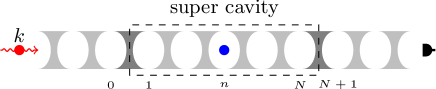
Figure 1: (Color online). Schematic configuration of the single-photon scattering problem for the 1D CCA model. A single photon (filled red circle) with the wave vector $k$ injects from the left side of the super cavity composed of $N$ cavities, which is formed by a relatively small coupling strength $\eta$ with the outside cavities. A two-level atom (filled blue circle) is in the $n$-th cavity of the SC. The transmission spectrum is measured by the detector on the right side of the SC. Here we take $N=5$ and $n=3$.

A tight-bonding model including five parts is introduced to describe the system

$$H=H_{S}+H_{L}+H_{R}+H_{SL}+H_{SR},$$ (1)

where

$$H_{S} = \sum^{N}_{j=1}\omega_{c}a^{{\dagger}}_{j}a_{j}+\sum^{N}_{j=2}\xi(a^{{\dagger}}_{j-1}a_{j}+a^{{\dagger}}_{j}a_{j-1})$$ (2)

$$+\omega_{a}|e\rangle\langle e|+g(a^{{\dagger}}_{n}\sigma^{-}+\mathrm{H.c.}),$$

$$H_{L} = \sum^{0}_{j=-\infty}[\omega_{c}a^{{\dagger}}_{j}a_{j}+\xi(a^{{\dagger}}_{j-1}a_{j}+a^{{\dagger}}_{j}a_{j-1})],$$ (3)

$$H_{R} = \sum^{\infty}_{j=N+1}[\omega_{c}a^{{\dagger}}_{j}a_{j}+\xi(a^{{\dagger}}_{j}a_{j+1}+a^{{\dagger}}_{j}a_{j+1})],$$ (4)

$$H_{SL} = \eta(a^{{\dagger}}_{0}a_{1}+\mathrm{H.c.}),$$ (5)

$$H_{SR} = \eta(a^{{\dagger}}_{N}a_{N+1}+\mathrm{H.c.}).$$ (6)

Here $H_{S}$ describes the SC system, $H_{L}$ ($H_{R}$) describes the left (right) channel that is formed by the segment of the cavity array left (right) to the SC, and $H_{SL}$ ($H_{SR}$) describes the interaction between the SC with the outsides. $a^{{\dagger}}_{j}$ ($a_{j}$) is the photon creation (annihilation) operator for the $j$-th single-mode cavity, $|e\rangle$ ($|g\rangle$) is the excited (ground) state of the atom, and $\sigma^{-}$($\sigma^{+}$) is the atomic lowering (raising) operator. $\omega_{c}$ is the intrinsic frequency of each single-mode cavity, $\omega_{a}$ is the transition frequency of the two-level atom, and $g$ is the coupling strength between the cavity and the atom. $\xi$ is the coupling strength between neighboring cavities in the SC, the left channel and the right channel, while $\eta$ is the coupling strength of neighboring cavities between them. In addition, we require that $\eta\ll\xi$, and set $\hbar=1$ throughout this paper.

The basic task here is to investigate the single photon scattering problem. When a single photon with wave vector $k$ injects from the left channel towards the SC system, what is the transmission spectrum obtained in the right channel?

Now the scattering state can be expanded as

$$|\Psi_{k}\rangle=|\phi_{k}\rangle+r|\phi_{k}^{\ast}\rangle+t|\vartheta_{k}\rangle+\sum^{N}_{j=1}d_{j}|j\rangle+\lambda|e\rangle,$$ (7)

where

$$|\phi_{k}\rangle = \sum^{0}_{j=-\infty}e^{ikj}|j\rangle,$$ (8)

$$|\vartheta_{k}\rangle = \sum^{+\infty}_{j=N+1}e^{ikj}|j\rangle,$$ (9)

with $|j\rangle=a_{j}^{\dagger}|G\rangle$ and $|e\rangle=\sigma^{+}|G\rangle$. Here, $|G\rangle=|vac;g\rangle$ represents the state with all the cavities in their vacuum states while the atom in the ground state. In Eq. (7), the coefficients $r$ and $t$ are the reflection and transmission amplitudes respectively, $d_{j}$ is the probability amplitude for finding the photon in the $j$-th cavity, and $\lambda$ is the probability amplitude for the atom in the excited state. The scattering state satisfies the stationary Schrödinger equation

$$H|\Psi_{k}\rangle=E_{k}|\Psi_{k}\rangle.$$ (10)

In general, the transmission amplitude $t$ is completely determined by Eq.(10), and the transmission rate $T={|t|}^{2}$ can be obtained. One of our main theoretical results is

$$t=\frac{ie^{-i(k+\pi)(N+1)}2\gamma^{2}\sin k}{e^{-2ik}|A_{N}^{n}|+\gamma^{2}e^{-ik}(|A_{N-1}^{n}|+|A_{N-1}^{n-1}|)+\gamma^{4}|A_{N-2}^{n}|},$$ (11)

where $\gamma=\eta/\xi$, and $A_{N}^{n}=[H_{S}(N,n)-E_{k}]/\xi$, with the dispersion relation $E_{k}=\omega_{c}+2\xi\cos k$ (the wave vector $k$ is dimensionless by setting the distance between arbitrary two neighbouring cavities as unit), $H_{S}(N,n)$ is the Hamiltonian of the SC system with $N$ cavities and the two-level atom in the $n$-th cavity, $|A_{N}^{n}|$ is the determinant of $A_{N}^{n}$. The detailed derivation of Eq.(11) is given in the Appendix.

Since $\gamma$ is a small parameter, the transmission peaks occur only when $|A_{N}^{n}|$ is small at least in the order of $\gamma^{2}$. In addition, $|A_{N}^{n}|=0$ only when $E_{k}$ is the eigen-energy of the SC system. Therefore, the necessary condition to observe the transmission peaks is that $E_{k}$ is near resonant with the eigen-modes of the SC system.

III Single photon scattering with empty super cavity

As the first step, we study the transmission spectrum for the SC without the two-level atom, i.e., an empty SC. As is well known, the eigenvalues and eigenstates of the empty SC are

$$\nu_{m} = \omega_{c}+2\xi\cos(j\theta_{m}),$$ (12)

$$|\Phi_{m}\rangle = \sqrt{\frac{2}{N+1}}\sum^{N}_{j=1}\sin(j\theta_{m})|j\rangle,$$ (13)

where $\theta_{m}=\frac{m\pi}{N+1}$ with $m$ being any integer between $1$ and $N$.

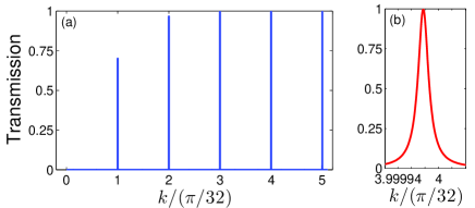
Figure 2: (Color online). (a) The transmission rate vs the incident wave vector $k$ for the empty SC. Only the first five transmission peaks are shown. (b) Zoom in of the $4$-th transmission peak. Here we choose the parameters $N=31$, $\xi=1$, and $\eta=0.01$.

Then the peaks in the transmission spectrum shall appear near the resonance $E_{k}=\nu_{m}$, i.e. $k=\theta_{m}$, which is numerically demonstrated in Fig. 2(a). In the figure, we only show the first five peaks, where the fourth peak is zoomed in in Fig. 2(b). It is apparent that each peak has a non-zero width which means the corresponding electromagnetic mode in the SC system has finite lifetime due to the dissipation arising from the coupling with the left and right channels. In other words, the left and right channels act not only as the carriers of the scattering waves, but also as the dissipation reservoirs of the SC.

As demonstrated above, the numerical results show that the SC is essentially an $N$-mode cavity, and every eigen-mode of the SC has a relatively long life time. In what follows, we will study how a single two-level atom that couples with the SC can dramatically change the transmission spectrum, and investigate the effects induced by the multi-mode cavity fields.

IV Single photon scattering with one atom in the super cavity

When a two-level atom interacts with the $n$-th cavity, it is convenient to rewrite the Hamiltonian $H_{S}$ in the eigen-modes of the SC as

$$H_{S}=\sum_{k}\nu_{k}b_{k}^{\dagger}b_{k}+\omega_{a}|e\rangle\langle e|+\sum_{k}g_{k}(b_{k}^{\dagger}\sigma_{-}+b_{k}\sigma_{+}),$$ (14)

where

$$b^{{\dagger}}_{k} = \sqrt{\frac{2}{N+1}}\sum^{N}_{j=1}\sin(j\theta_{k})a^{{\dagger}}_{j},$$ (15)

$$g_{k} = g\sqrt{\frac{2}{N+1}}\sin(j\theta_{k}).$$ (16)

Note that the coupling strength $g_{k}$ depends on the location of the atom and the length of the SC. It is the standard model of cavity QED in the multi-mode setting.

When the frequency of the atom is near resonant with a pre-selection $k^{\ast}$th mode of the SC, we may adopt the single mode approximation for the SC. Then the two relative eigen-energy levels are

$$E_{k\pm}=\frac{\nu_{k^{\ast}}+\omega_{a}}{2}\pm\frac{\Delta_{k^{\ast}}}{2},$$ (17)

where the vacuum Rabi splitting is

$$\Delta_{k^{\ast}}=\sqrt{(\nu_{k^{\ast}}-\omega_{a})^{2}+4g_{k^{\ast}}^{2}}.$$ (18)

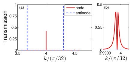
Figure 3: (Color online). (a) Transmission rates vs the incident wave vector (just around the resonant mode). Blue dashed and red solid line each stands for the atom at the antinode (n=12) or node (n=8) of the mode. (b) Zoom in of of the red peak. Here the atom is near resonant with the $4$-th mode of the SC with $\omega_{a}=1.847760755\xi$, and $g=0.1$.

Now we numerically check the validness of the above single mode approximation. First, we plot the transmission spectrum when the two-level atom is located at the node and antinode of the resonant mode of the SC, which is shown in Fig. 3 (a). When the atom is located at the antinode of the resonant mode, the obvious vacuum Rabi splitting appears. When the atom is located at the node, i.e., the two-level atom does not interact with the resonant mode of the SC, no vacuum Rabi splitting is observed as expected. However, the peak is lower than $1/2$ in the latter case. If the single mode approximation is valid, then the two-level atom without interacting with the resonant mode of the SC will not affect the transmission rate. In other words, it is expected to be similar to the case shown in Fig. 2(b). Thus we plot the zoom in for the case of the atom at the node as shown in Fig. 3(b). Obviously, the transmission spectrum shown in Fig. 2 (b) exhibits an obvious valley exactly at the resonant mode of the SC, which is essentially different from Fig. 7(b).

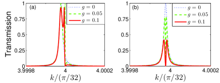
Figure 4: (Color online). Transmission spectrum for the atom at the node of the resonant mode with $g=0$ (blue dotted line), $g=0.05$ (green dashed line) and $g=0.1$ (red solid line). (a) $\omega_{a}=\nu_{4}$ . (b) $\omega_{a}=1.847760755\xi$.

To investigate the physics underlying the transmission spectrum shown in Fig. 3(b), the frequency of the atom is tuned to be resonant with the mode while keeping the atom at the node, the transmission spectrum is given for different coupling strength $g$ as shown in Fig. 4(a). When $g=0$, we recover the transmission spectrum shown in Fig. 2(b). For $g$ is not $0$, a second peak appears near the frequency of the atom. Since the atom does not couple with the resonant mode, the peak must be originated from the atom coupling with the non-resonance modes. We assert that due to the different influence of the outsides, the transmission spectrum for each channel independently is partially overlap at resonant condition which leads to the above mentioned transmission spectrum as shown in next section. By increasing $g$, the transmission peak becomes wider as expected. The numerical result in Fig. 4(a) clearly shows that in the case of the atom located at the node of the resonant mode, two channels exist for the photon transmitting through the SC, one is the resonant cavity while the other is result from the atom coupling with the non-resonance modes.

Further in Fig. 4(b), we tune the frequency of the atom so that the transmission peaks for the two channels coincides as shown in next section. However, we find that the single photon is completely reflected at the original transmission peak of the resonant mode, which implies the transmission amplitudes through the two channels interfere destructively. The appearance of the transmission valley comes from the different widths of the transmission peaks from the two channels. Moreover, the widths of the valleys are determined by the coupling strength $g$, and it further confirms the existence of quantum interference. A more physical explanation of the transmission spectrum is given in the next section to intuitively show the mechanism behind the transmission dip.

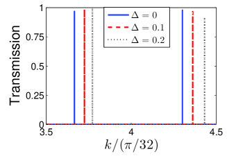
Figure 5: (Color online). Transmission spectrum for different detunings when the atom located in the antinode. Here we give the results for $\Delta=\omega_{a}-\nu_{4}=0$ (blue solid line), $\Delta=0.01\xi$ (red dashed line), and $\Delta=0.02\xi$ (black dotted line).

As discussed above, the non-resonance modes dramatically change the transmission spectrum when the atom is located at the node, so a natural problem is how the non-resonance modes affect the transmission spectrum when the two-level atom is located at the antinode of the resonant mode. To this end, we plot the transmission spectrum for different detuning when the atom is located at the antinode as shown in Fig. 5. We show that, by tuning the frequency of the atom higher than the resonant mode, the peak of high frequency will move away faster than the one with low frequency, and the opposite behavior can be seen if tuning the atom frequency lower. Obviously, this behavior can not be explained by the single mode approximation, and must be resorted to the effects of non-resonance modes of the SC. Notice that the similar phenomenon is mentioned in Ref. 11 .

V Physical explanation of the transmission valley in the two level approximation

Now let us give a more detailed and physical explanation about the transmission valley shown in Fig 4. As we know, the energy levels of the SC that are near resonant with the energy of the incoming photon dominates the photon transmission through the SC. In the cases that the transmission valley occurs, there are two energy levels of the SC that are near resonant with the energy of the incoming photon, one is the near resonant mode of the SC that does not interact with the atom, the other is the atomic excited state dressed by the non-resonance modes. So it is reasonable to maintain only these two levels in the Hamiltonian $H_{S}$, which is called the two level approximation. In the two level approximation, the Hamiltonian of our system can be written as $H=H_{S}+H_{L}+H_{R}+H_{SL}+H_{SR}$ with $H_{L}$ and $H_{R}$ the same as in the exact model and

$$H_{S} = \nu_{m}|\psi_{m}\rangle\langle\psi_{m}|+\omega_{A}|\varphi_{m}\rangle\langle\varphi_{m}|,$$ (19)

$$H_{SL} = \eta\left[(\alpha_{1}|0\rangle\langle\psi_{m}|+\beta_{1}|0\rangle\langle\varphi_{m}|)+\mathrm{H.c.}\right],$$ (20)

$$H_{SR} = \eta\left[(\alpha_{2}|N+1\rangle\langle\psi_{m}|+\beta_{2}|N+1\rangle\langle\varphi_{m}|)+\mathrm{H.c.}\right],$$ (21)

where $|\psi_{m}\rangle=b^{{\dagger}}_{m}|G\rangle$ $\alpha_{1}=\langle 1|\psi_{m}\rangle$, $\beta_{1}=\langle 1|\varphi_{m}\rangle$, $\alpha_{2}=\langle N|\psi_{m}\rangle$, and $\beta_{2}=\langle N|\varphi_{m}\rangle$. $\omega_{A}$ is the eigen-energy of the atomic state.

Now the scattering state can be expanded as

$$|\Psi_{k}\rangle=|\varphi_{k}\rangle+r|\varphi_{k}^{\ast}\rangle+t|\vartheta_{k}\rangle+\mu|\psi_{m}\rangle+\zeta|\varphi_{m}\rangle$$ (22)

with $\mu$ and $\zeta$ being the excitation amplitudes of the modes $|\psi_{m}\rangle$ and $|\varphi_{m}\rangle$, respectively.

The stationary Schrödinger equation $H|\Psi_{k}\rangle=E_{k}|\Psi_{k}\rangle$ results in the following set of scattering equations

$$\omega_{c}r^{{}^{\prime}}+\xi(e^{-ik}+re^{ik})+\eta(\alpha_{1}\mu+\beta_{1}\zeta) = E_{k}r^{{}^{\prime}}$$ (23)

$$\eta[r^{{}^{\prime}}\alpha_{1}+t^{{}^{\prime}}\alpha_{2}]+\nu_{m}\mu = E_{k}\mu$$ (24)

$$\eta[r^{{}^{\prime}}\beta_{1}+t^{{}^{\prime}}\beta_{2}]+\omega_{A}\zeta = E_{k}\zeta$$ (25)

$$\omega_{c}t^{{}^{\prime}}+\eta(\alpha_{2}\mu+\beta_{2}\zeta)+\xi t^{{}^{\prime}}e^{ik} = E_{k}t^{{}^{\prime}}$$ (26)

and the transmission rate $T=|t|^{2}$ can be determined. Here, we set $t^{{}^{\prime}}=te^{ik(N+1)}$ and $r^{{}^{\prime}}=1+r$.

From Eq. (35), the condition for the perfect reflection is

$$\alpha_{2}\mu+\beta_{2}\nu=0.$$ (27)

Eq. (27) can be understood as follows. When the three levels $|\psi_{m}\rangle$, $|\varphi_{m}\rangle$, and $|N+1\rangle$ are considered, the state $\mu|\psi_{m}\rangle+\zeta|\varphi_{m}\rangle$ is the dark state relative to $|N+1\rangle$ as in the EIT setting. This shows the interference mechanism behind the transmission valley and is the central point to understand the phenomenon.

V.1 Analytical and numerical results for $\omega_{a}=\nu_{m}$

When the atom is resonant with the $m$-th mode of the cavity ($\omega_{a}=\nu_{m}$), the state $|\varphi_{m}\rangle$ with eigen-energy $\omega_{A}=\omega_{a}$ can be analytically expressed as

$$|\varphi_{m}\rangle=c_{m}^{{\dagger}}|G\rangle+d_{m}^{{\dagger}}|G\rangle-\frac{1+\gamma}{g\sqrt{A}}\sin{\theta_{m}}|e\rangle,$$ (28)

where

$$c_{m}^{{\dagger}} = \frac{1}{\sqrt{A}}\sum^{n}_{j=1}\sin(j\theta_{m})a_{j}^{\dagger},$$

$$d_{m}^{{\dagger}} = -\frac{\gamma}{\sqrt{A}}\sum^{N}_{j=n+1}\sin(j\theta_{m})a_{j}^{\dagger},$$

$$\gamma = n/(N-n+1),$$

$$A = \sqrt{\frac{N+1}{N-n+1}\left[\frac{n}{2}+\frac{N+1}{g^{2}(N-n+1)}\sin^{2}{\theta_{m}})\right]}.$$

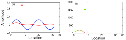
Figure 6: (Color online). (a) Blue (red) solid line and triangle each represents the excitation amplitude of the SC and the atom as in state $|\psi_{m}\rangle$ ($|\varphi_{m}\rangle$). (b) Green dashed (red solid)line and triangle (circle) each represents the excitation amplitude of the SC and the atom as in state $|\Psi_{m}\rangle_{SC}$ in the two level approximation model (the exact model). Here, $g=0.05$ and $m=4$ while all the other parameters are the same as before.

The states $|\psi_{m}\rangle$ and $|\varphi_{m}\rangle$ are demonstrated in Fig. 6(a). In addition, a simple calculation shows the perfect reflection appears at $E_{k}=\nu_{m}$. Then the analytical result of the scattering state within the SC

$$|\Psi_{m}\rangle_{SC}=C\left[\sqrt{\frac{2}{N+1}}\sin(N\theta_{m})c_{m}^{{\dagger}}|G\rangle+\frac{\alpha_{2}\sin{\theta_{m}}}{g\sqrt{A}}|e\rangle\right],$$ (29)

where

$$C=-\frac{2i(\gamma+1)\sin{\theta_{m}}}{\eta(\alpha_{1}\beta_{2}-\alpha_{2}\beta_{1})}.$$

The state is clearly localized between the atom and the left end of SC, while the two modes represented by $|\psi_{m}\rangle$ and $|\varphi_{m}\rangle$ are extended through out the SC (as clearly shown in Fig 6).

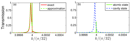
Figure 7: (Color online). Transmission rates vs the incident wave vector for different model. (a) The results under the full Hamiltonian (red solid line) and two level approximation (green dashed line). (b) The results when we only consider one channel which is supported by the $m$th eigen-state of the SC (blue dashed line) and the atomic state (green solid line).

To test the validness of the two level approximation, we compare the numerical results in the approximation with those from the exact model. As shown in Fig. 7(a), the transmission spectrum from the two level approximation agrees well with those from the exact model, which verifies that the transmission valley is a two level effect. To further clarify the two level approximation, we give the transmission spectrum when either one of the two levels is considered, which is shown in Fig. 7(b). Obviously, the transmission valley just appears in the overlap region due to quantum interference.

V.2 Numerical results for $\omega_{a}\neq\nu_{m}$

When the atom is near resonant with the $m$-th mode of the SC, the analytical expression for the state $|\varphi_{m}\rangle$ is difficult to obtain. Then we numerically evaluate the state $|\varphi_{m}\rangle$ and the eigen-energy $\omega_{A}$. The transmission spectrum within the two level approximation is shown in Fig. 8(a). As before, we also compare these approximate results with those from the exact model, and find that the approximation is quite accurate. The transmission spectrum from either one of the two levels are shown in Fig 8(b), which verifies that the transmission valley comes from the quantum interference between the two channels assisted by the two levles.

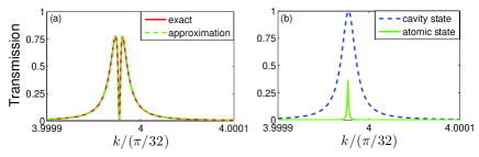
Figure 8: (Color online). Transmission spectrum for various channels. The transition frequency of the atom $\omega_{a}=1.847760755\xi$. (a) Blue dashed line: the cavity state $|\psi_{m}\rangle$. Green solid line: the atomic state $|\varphi_{m}\rangle$. (b) Green dashed line: the two level approximation. Red solid line: the exact model.

VI Remarks and Conclusion

In this paper, we have studied the single-photon scattering in a typical CCA system. Experimentally, the CCA can be realized by the superconducting transmission line resonators which supports the single mode microwave electromagnetic field with the resonant frequency $\omega_{c}/2\pi\approx 3$ GHz Wallraff . The coupling between neighboring resonators can be realized by via the tunable capacitances and its strength can be achieved $\xi(\eta)/2\pi=5-100$ MHz Wallraff ; Mariantoni . Correspondingly, the two-level atom can be realized by the superconducting qubit such as flux qubit whose transition frequency can be tuned by readily adjusting the flux through the loop, and the coupling strength between the qubit and the resonator can be achieved $g\approx 0.12\omega_{c}$ in a recent experimental scheme TN .

In conclusion, we propose a simple microscopic model of cavity QED based on CCA, and prove that the transmission peaks shall appear near the eigenvalues of the whole SC system. One of the advantages of this model is that it provides a platform to deal with the non-resonance modes in the microscopic level. Firstly we show that the SC composed by a segment of 1D cavity array is a multi-mode cavity by studying the transmission spectrum through an empty SC. Then we study the multi-mode effects in the SC system by investigating the transmission spectrum for the SC interacting with a two-level atom, located at the antinode or node of a pre-selected resonant mode of SC. When the atom locates at the antinode, we observe the vacuum Rabi splitting in the transmission spectrum as expected. However, when the two-level atom locates at the node of the near resonant mode, we find a valley in the transmission spectrum, which can be explained by the interference of the transmission amplitude through two channels, one channel is the resonant mode, the other is the atomic excited state dressed by the non-resonance modes. We hope this model can enlighten the study of multi-mode effects in cavity QED.

APPENDIX: LOCATIONS OF THE PEAKS

By comparing the coefficients of $\{|j\rangle\}$ and $|e\rangle$ in the stationary scattering equation (10), we obtain

$$E_{k}=\omega_{c}+2\xi\cos k,$$ (30)

and

$$\omega_{c}r^{{}^{\prime}}+\xi(e^{-ik}+re^{ik})+\eta d_{1} = E_{k}r^{{}^{\prime}},$$ (31)

$$\omega_{c}d_{1}+\eta r^{{}^{\prime}}+\xi d_{2} = E_{k}d_{1},$$ (32)

$$\omega_{c}d_{j}+\xi(d_{j-1}+d_{j+1}) = E_{k}d_{j},$$ (33)

$$\omega_{c}d_{n}+\xi(d_{n-1}+d_{n+1})+\lambda g = E_{k}d_{n},$$ (34)

$$\lambda\omega_{a}+gd_{n} = \lambda E_{k},$$ (35)

$$\omega_{c}d_{N}+\xi d_{N-1}+t^{{}^{\prime}}\eta = E_{k}d_{N},$$ (36)

$$\omega_{c}t^{{}^{\prime}}+\eta d_{N}+\xi t^{{}^{\prime}}e^{ik} = E_{k}t^{{}^{\prime}}.$$ (37)

where $2\leq j\leq N-1$ and $j\neq n$.

For $\omega_{a}\neq E_{k}$, Eq. (35) leads to

$$\lambda=\frac{g}{E_{k}-\omega_{a}}d_{n}.$$ (38)

Substituting Eq. (38) into Eq. (34), we have

$$(\omega_{c}+\frac{g^{2}}{E_{k}-\omega_{a}})d_{n}+\xi(d_{n-1}+d_{n+1})=E_{k}d_{n}.$$ (39)

We introduce the following parameters:

$$d_{0} = 1+r,$$ (40)

$$d_{N+1} = te^{ik(N+1)},$$ (41)

$$\alpha = \frac{\omega_{c}-E_{k}}{\xi}=-e^{ik}-e^{-ik},$$ (42)

$$\beta = \frac{\omega_{c}-E_{k}+\frac{g^{2}}{E_{k}-\omega_{a}}}{\xi}=\alpha+\frac{g^{2}}{\xi(E_{k}-\omega_{a})},$$ (43)

$$\gamma = \frac{\eta}{\xi},$$ (44)

$$\delta = e^{ik}-e^{-ik}.$$ (45)

Then the scattering equation can be expressed in the following matrix form

$$\left(\begin{array}[]{ccccccccccc}\alpha+e^{ik}&\gamma&&&&&&&&&\\ \gamma&\alpha&1&&&&&&&&\\ &1&\alpha&1&&&&&&&\\ &&&\ddots&&&&&&&\\ &&&1&\alpha&1&&&&&\\ &&&&1&\beta&1&&&&\\ &&&&&1&\alpha&1&&&\\ &&&&&&&\ddots&&&\\ &&&&&&&1&\alpha&1&\\ &&&&&&&&1&\alpha&\gamma\\ &&&&&&&&&\gamma&\alpha+e^{ik}\end{array}\right)\left(\begin{array}[]{c}d_{0}\\ d_{1}\\ d_{2}\\ \vdots\\ d_{n-1}\\ d_{n}\\ d_{n+1}\\ \vdots\\ d_{N-1}\\ d_{N}\\ d_{N+1}\end{array}\right)=\left(\begin{array}[]{c}\delta\\ 0\\ 0\\ \vdots\\ 0\\ 0\\ 0\\ \vdots\\ 0\\ 0\\ 0\end{array}\right),$$ (46)

which is abbreviated as

$$BD=\Gamma$$ (47)

with

$$B=\left(\begin{array}[]{ccc}\alpha+e^{ik}&\gamma&\\ \gamma&A^{n}_{N}&\gamma\\ &\gamma&\alpha+e^{ik}\\ \end{array}\right)$$ (48)

and

$$A^{n}_{N}=\frac{H_{S}-E_{k}}{\xi}.$$ (49)

By applying the Cramer’s Rule, the transmission amplitude is

$$t=e^{-ik(N+1)}d_{N+1}=e^{-i(k+\pi)(N+1)}\frac{\delta\gamma^{2}}{|B|}$$ (50)

with $|B|$ the determinant of the matrix. From Eq. (48), $|B|$ can be analytical expressed as

$$|B|=e^{-2ik}|A^{n}_{N}|+e^{-ik}\gamma^{2}(|A^{n-1}_{N-1}|+|A^{n}_{N-1}|)+\gamma^{4}|A^{n-1}_{N-2}|.$$ (51)

As mentioned before $\eta\ll\xi$, leads to $\gamma\ll 1$. So in order to gain large transmission probability, $|A^{n}_{N}|$ in the denominator of Eq. (51) must be small at least in the order of $\gamma^{2}$, which clearly shows that the transmission peaks should be achieved just near the eigenvalues of the SC system. This result is easy to generalize to multi-atom situation.

References

- (1) E. M. Purcell, Phys. Rev. 69, 681(1946).
- (2) R. J. Thompson, G. Rempe, and H. J. Kimble, Phys. Rev. Lett. 68, 1132(1992).
- (3) M. Brune, F. Schmidt-Kaler, A. Maali, J. Dreyer, E. Hagley, J. M. Raimond, and S. Haroche, Phys. Rev. Lett. 76, 1800(1996).
- (4) R. Rlsberger, K. Schlage, B. Sahoo, S. Couet, R. Rfer, Science 328, 1248 (2010).
- (5) M. Mcke, E. Figueroa, J. Bochmann, C. Hahn, K. Murr, S. Ritter, C. J. Villas-Boas, and G. Rempe, Nature 465, 755 (2010).
- (6) D. G. Angelakis, M. F. Santos, and S. Bose, Phys. Rev. A 88, 013832 (2013).
- (7) M. J. Hartmann, F. G. S. L. Brandaõ, and M. B. Plenio, Nat. Phys. 2 849 (2006).
- (8) A. D. Greentree, C. Tahan, J. H. Coleand, and L. C. L. Hollenberg, Nat. Phys. 2 856 (2006).
- (9) A. Kay and D. G. Angelakis, Europhys. Lett.84, 20001 (2008).
- (10) J. Cho, D. G. Angelakis, and S. Bose, Phys. Rev. Lett.101, 246809 (2008).
- (11) J. Koch, A. A. Houck, K. L. Hur, and S. M. Girvin, Phys. Rev. A 82, 043811 (2010).
- (12) M. Hafezi, E. A. Demler, M. D. Lukin, and J. M. Taylor, Nat. Phys. 7, 907 (2011).
- (13) L. Zhou, Z. R. Gong, Y. X. Liu, C. P. Sun, and F. Nori, Phys. Rev. Lett. 101, 100501(2008).
- (14) Z. R. Gong, H. Ian, L. Zhou, and C. P. Sun, Phys. Rev. A 78, 053806 (2008).
- (15) D. Z. Xu, Y. Li, C. P. Sun, and P. Zhang,Phys. Rev. A 78, 053806 (2008).
- (16) L. Zhou, Y. Chang, H. Dong, L. M. Kuang, and C. P. Sun, Phys. Rev. A 85, 013806(2012).
- (17) J. T. Shen and S. Fan, Phys. Rev. Lett. 95, 213001 (2005).
- (18) A. Wallraff, D. I. Schuster, A. Blais, L. Frunzio, R. S. Huang, J. Majer, S. Kumar, S. M. Girvin, and R. J. Schoelkopf, Nature 431, 162 (2004).
- (19) M. Mariantoni, F. Deppe, A. Marx, R. Gross, F. K. Wilhelm, and E. Solano, Phys. Rev. B 78, 104508 (2008).
- (20) T. Niemczyk, F. Deppe, H. Huebl, E. P. Menzel, F. Hocke, M. J. Schwarz, J. J. Garcia-Ripoll, D. Zueco, T. Hümmer, E. Solano, A. Marx, and R. Gross, Nat. Phys. 6, 772 (2010)