DGFIndex for Smart Grid: Enhancing Hive with a Cost-Effective Multidimensional Range Index

Abstract

In Smart Grid applications, as the number of deployed electric smart meters increases, massive amounts of valuable meter data is generated and collected every day. To enable reliable data collection and make business decisions fast, high throughput storage and high-performance analysis of massive meter data become crucial for grid companies. Considering the advantage of high efficiency, fault tolerance, and price-performance of Hadoop and Hive systems, they are frequently deployed as underlying platform for big data processing. However, in real business use cases, these data analysis applications typically involve multidimensional range queries (MDRQ) as well as batch reading and statistics on the meter data. While Hive is high-performance at complex data batch reading and analysis, it lacks efficient indexing techniques for MDRQ.

In this paper, we propose DGFIndex, an index structure for Hive that efficiently supports MDRQ for massive meter data. DGFIndex divides the data space into cubes using the grid file technique. Unlike the existing indexes in Hive, which stores all combinations of multiple dimensions, DGFIndex only stores the information of cubes. This leads to smaller index size and faster query processing. Furthermore, with pre-computing user-defined aggregations of each cube, DGFIndex only needs to access the boundary region for aggregation query. Our comprehensive experiments show that DGFIndex can save significant disk space in comparison with the existing indexes in Hive and the query performance with DGFIndex is 2-50 times faster than existing indexes in Hive and HadoopDB for aggregation query, 2-5 times faster than both for non-aggregation query, 2-75 times faster than scanning the whole table in different query selectivity.

1 Introduction

With the development of the Smart Grid, more and more electric smart meters are deployed. Massive amounts of meter data are sent to centralized systems, like Smart Grid Electricity Information Collection System, at fixed frequencies. It is challenging to store these data and perform efficient analysis, which leads to the smart meter big data problem. For example, currently 17 million smart meters are deployed in the Zhejiang Province, which will be increased to 22 million in next year. As required by the standard of the China State Grid, each of them will generate meter data once every 15 minutes (96 times a day). Even only in a single table of electric quantity, there will be 2.1 billion records needed to be stored and analyzed effectively daily.

The traditional solution in the Zhejiang province was based on a relational database management system (RDBMS). It implements its analysis logics using SQL stored procedures, and builds many indexes internally to improve the efficiency of selective data reading. It is observed that global statistics on big tables lead to poor performance, and the throughput of data writing is fairly low due to the indexes used in the database system. With the increasing of the number of metering devices and collection frequency, this situation becomes more dramatic and the capacity of the current solution is reached. Since traditional RDBMS exhibits weak scalability and unsatisfied performance on big data. On top of that it is also surprisingly expensive for business users to deploy a commercial parallel database. Hadoop [2], an open source implementation of MapReduce [12] and GFS [17] allows users to run complex analytical tasks over massive data on large commodity hardware clusters. Thus, it also is a good choice for the Zhejiang Grid. Furthermore, Hive [25, 5], a warehouse-like tool built on top of Hadoop that provides users with an SQL-like query language, is also adopted, making it easier to develop and deploy big data applications. As observed in our experiences in Zhejiang Grid, because of the excellent scalability and powerful analysis ability, Hive on top of Hadoop demonstrates its superiority in term of high throughput storage, high efficient batch reading and analyzing of big meter data. The problem is that, due to the lack of efficient multidimensional indexing in Hive, the efficiency of MDRQ processing becomes a new challenge.

Current work on indexes on HDFS either focuses on one-dimensional indexes [13, 16], or mainly for spatial data type, such as point, rectangle or polygon [15, 11]. They both can not perform effective multidimensional range query processing on non-spatial meter data. Currently, Hive features three kinds of indexes internally, the Compact Index, the Aggregate Index, and the Bitmap Index, which can get relevant splits according to the predicates of a query. These existing indexes are stored as a table in Hive containing every index dimension and an array of locations of corresponding records. As the number of index dimensions increases, the index table becomes very large. It will occupy a large amounts of disk space and result in low performance of MDRQs, as Hive first scans the index table before processing.

With our observation of the meter data and queries in smart grid, we find that it has some particular features mostly happen in general IoT (Internet of Things) system: (i) Because the collected data is directly related to physical events, there is always a time stamp field in a record. (ii) Since meter data is a fact from physical space, it becomes unchanged after being verified and persisted in database. (iii) Since the change of the schema of meter data means carefully redesign of the system, and will definitely lead to complicate redeployment or at least reconfiguration of all end devices, the schema is almost static in a fairly long period of time. (iv) Since the business logic may require to add some constraints on more than one data column, many queries contain MDRQ characteristics. (v) Most of the MDRQ queries are aggregation queries.

In this paper, taking advantage of the features of the meter data, we propose a distributed multidimensional index structure named DGFIndex (Distributed Grid File Index), which uses grid file to divide the data space into small cubes [22]. With this method, we only need to store the information of the cubes instead of every combination of multiple index dimensions. This results in a very small index size. Moreover, by storing the index in form of key-value pairs and cube-based pre-computing techniques, the processing of MDRQ in Hive is highly improved. Our contributions are three-fold: (i) We share the experience of deploying Hadoop in Smart Grid and transforming legacy applications to Hadoop-based applications. We analyze and summarize the existing index technologies used in Hive, and point out their weakness on MDRQ processing, which implies the essential requirement for multiple dimensional index in traditional industry . (ii) We propose a distributed grid file index structure named DGFIndex, which reorganizes data on HDFS according to the splitting policy of grid file(Thus, each table can only create one DGFIndex). DGFIndex can filter unrelated splits based on predicate, and filter unrelated data segments in each split. Moreover, with pre-computing technique, DGFIndex only needs to read less data than query-related data. With above techniques, DGFIndex improves greatly the performance of processing MDRQ in Hive. (iii) We conduct extensive experiments on large scale real-world meter data workloads and TPC-H workloads. The results demonstrates the improved performance of processing MDRQs using DGFIndex over existing indexes in Hive and HadoopDB.

Compared with current indexes in Hive and other indexes on HDFS, DGFIndex’s advantages are: (i) Smaller index size can accelerate the speed of accessing index and improve the query performance. (ii) For aggregation query, DGFIndex can efficiently perform it by only scanning the boundary of query region and directly get the pre-computed value of the inner query region. (iii) By making use of the time stamp difference and setting the time stamp of collecting data as the default index dimension, DGFIndex does not need to update or rebuild after inserting more data, which makes sure that the writing throughput will not be influenced by existence of DGFIndex.

The rest of the paper is organized as follows. In Section 2, we give details of the big smart meter data problem and introduce the existing indexes in Hive. In Section 3, we will share the experience of transforming traditional legacy system to cost effective Hadoop based system. In Section 4, we describe DGFIndex, and give details on its architecture, the index construction, and how it is used in the MDRQ process. Section 5 discusses our comprehensive experiment results in detail. Section 6 shows some findings and practical experience about the existing indexes in Hive. Section 7 presents related work. Finally, Section 8 concludes the paper with future work.

2 Background

In this section, we will give an overview of the Big Smart Meter Data Problem and introduce the Hive architecture and Hive’s indexes.

2.1 The Big Smart Meter Data Problem

To make electric power consumption more economic, electric power companies and grid companies are trying to improve the precision of their understanding of the demand of power and the trend of power consumption for increasing time frames. In recent years, the development and broad adaption of smart meters makes it possible to collect meter data multiple times every day. By analyzing these data, electric power companies and grid companies can get valuable information about continuous, up-to-date power consumption and figure out in time important business supporting results, like line loss rate, etc.

With the number of smart meters deployed and the frequency of data collection increasing, the amount of meter data becomes very large. The form of meter data record is illustrated in Figure 1. Each record of meter data consists of a user id, power consumption, collection date, positive active total electricity (PATE) with different rates, reverse active total electricity with different rates and various other metrics. The number of unique user ids is tens of millions in a province of China.

UserId	PowerConsumed	TimeStamp	PATE with Rate 1	Other Metrics
24012	12.34	1332988833	10.45	…

Figure 1: An Example of Meter Data Record

To get more statistical information, analysts need to perform many ad-hoc queries on these data. These queries have multidimensional range feature. For example, below are some typical queries:

• What was the average power consumption of user ids in the range 100 to 1000 and dates in the rangs ”2013-01-01” to ”2013-02-01”?

• How many users exist with a power consumption between 120.34 and 230.2 in the date range from ”2013-01-01” to ”2013-02-01”?

Additionally, many timing work flows are executed to analysis these meter data (stored procedures in previous RDBMS, will be described in Section 3). Many HiveQL predicates in these work flows have the same characteristics with the above ad-hoc queries. Thus, an efficient multidimensional range index is crucial for processing these queries in Hive.

2.2 Hive

Hive is a popular open-source data warehousing solution built on top of Hadoop. Hive features HiveQL, an SQL-like declarative language. By transforming HiveQL to a DAG (Directed Acyclic Graph) flow of MapReduce jobs, Hive allows users to run complex analysis expressed in HiveQL over massive data. When Hive reads the input table, it first generates a certain number of mappers based on the size of input table, every mapper processes a segment of the input table, which is named a split. Then, these mappers filter data according to the predicate of the query. Tables in Hive can be stored in different file formats, for example, plain text format (TextFile) and binary format (SequenceFile and RCFile [18]). Even though each file format can be compressed with different compression algorithms, Hive still has to scan the whole table without the help of index. This in turn results in large amounts of redundant I/O, and leads to high cost of resources and poor performance, especially for queries with low selectivity.

Index is a powerful technique to reduce data I/O and to improve query performance. Hive provides an interface for developers to add new index implementations. The purpose of an index in Hive is to reduce the number of input splits produced by the predicate in a query. As a result, the number of mappers will also be reduced. In the current version of Hive, there are three kinds of indexes, the Compact Index [8], the Aggregate Index [6], and the Bitmap Index [7]. All the three types are stored as a Hive table, and their purpose is to decrease the amount of data that needs to be read.

For the Compact Index, the schema of the index table is shown in Table 1. If the base table is not partitioned, Hive uses the HiveQL statement shown in Listing 1 to populate the index table. The INPUT_FILE_NAME represents the name of input file. The BLOCK_OFFSET_INSIDE_FILE represents the line offset in the TextFile format and the SequenceFile format and the block offset in the RCFile (not to be mistaken with the block in HDFS). Compact Index stores the position information of all combinations of multiple index dimensions of different data files.

⬇

INSERT OVERWRITE TABLE IndexTable

SELECT <index dimension list>,

INPUT_FILE_NAME,

collect_set(BLOCK_OFFSET_INSIDE_FILE)

FROM BaseTable

GROUP BY <index dimension list>,

INPUT_FILE_NAME

Listing 1: The Creation of a Compact Index

Table 1: Schema of a 3-Dimensional Compact Index

Column Name	Type
$index\ dimension\ 1$	$type\ in\ base\ table$
$index\ dimension\ 2$	$type\ in\ base\ table$
$index\ dimension\ 3$	$type\ in\ base\ table$
$\_bucketname$	$string$
$\_offset$	$array<bigint>$

An Aggregate Index is built on the basis of Compact Index, its purpose is to improve the processing of the GROUP BY query type. The user can specify pre-computed aggregations when creating an Aggregate Index (for now, only the $Count$ aggregation is supported). The schema of an Aggregate Index’ table includes additional pre-computed aggregations at the end of every line in a Compact Index table. The Aggregate Index uses the idea of index as data. Using query rewriting technique, it changes the GROUP BY query on the base table to a scan-based query over the smaller index table. Unfortunately, the use of Aggregate Indexes is heavily restricted: the dimensions that are referenced in SELECT, WHERE, and GROUP BY should be in the index dimensions, and the aggregations in a query should be in the pre-computed aggregation lists or can be derived from them.

The Bitmap Index is a powerful structure for indexing columns with a small amount of distinct values. In the RCFile format, except storing the offset of block, it stores the offset of every row in the block as a bitmap. In TextFile format, every line is seen as a block, so the offset of every row in the block is 0. Thus, Bitmap Index only improves the query performance on RCFile format data. A Bitmap Index changes the type of _offset in the compact index to bigint and adds a column _bitmaps with type array<bigint>.

Partition is another mechanism to improve query performance. Every partition is a directory in HDFS. It is similar to partitioning in a RDBMS. Partition can be seen as a coarse-grained index. The difference of partition with above indexes is that it needs to reorganize data into different directories.

When Hive processes query with Compact Index or Bitmap Index, it first scans the index table and writes relevant $filename-offsets$ pairs to a temporary file. Afterwards, the method $getSplits$ in $InputFormat$ reads the temporary file, and gets all splits from these file names in it. Finally, $getSplits$ filters irrelevant splits based on the offsets in temporary file.

Compact Index and Bitmap Index are used to filter unrelated splits, and Aggregate Index is used to improve the performance of GROUP BY queries. These three kinds of indexes have several limitations when processing MDRQs:

1. When the number of distinct values in every index dimensions is very large, the number of records in index table will be huge. The reason is that tables of these three types of indexes store all the combinations of each index dimensions. This leads to excessive disk consumption and, ultimately, a bad query performance.

2. When the records of an index dimension that have the same value are scattered evenly in the file (for example, every split has one record), these indexes will not filter any splits. The reason is that they do not reorganize data to put these records together, and their processing unit is split.

3. If the output temporary file of index is very big, it may overflow the memory of master, because the method $getSplits$ is run in a single master and it needs to load all information of the temporary file into memory before running MapReduce jobs.

Partitioning in Hive is not flexible, and when creating partitions for multiple dimensions, it will create a huge amount of directories. This will quickly overload the NameNode. In HDFS, all metadata about directories, files, and blocks are stored in the NameNode’s memory. The metadata of every directory occupies 150 bytes memory of NameNode [1]. For example, if we create partitions from three dimensions with 100 distinct values each, 1 million directories will be created, and 143 MB will be occupied in the NameNode’s memory, which is not including the metadata of files and blocks. However, partition is a good complement for index, because an index can be created on the basis of each partition.

3 Smart Grid Electricity Information Collection System

In this section, we will describe the data flow, system migration experience from a RDBMS-based system to a RDBMS and Hadoop/Hive-based system of the Electricity Consumption Information Collection System in Zhejiang Grid.

3.1 Data Flow in Zhejiang Grid

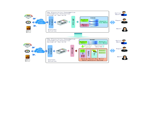
Figure 2: Previous Solution and Current Solution in Zhejiang Grid

Figure 2 shows the data flow abstraction in Zhejiang Grid. The smart meters are deployed in resident houses, public facilities and business facilities etc. The reporting frequency of smart meter can be set. The more frequent, the more precise. The reported meter data is transmitted by a information collector service to several queues. The clients of RDBMS then get the data from queues and write them into meter data tables in database.

In Zhejiang Grid, the data can be classified into three categories. The first one is meter data which is collected at fixed frequency. Its features are: (1) massive amounts of data, (2) a time stamp field in every record, (3) no changes are performed once meter data is verified and persisted into the database, and (4) the schema of meter data is almost static. The second category is archive data which records the detailed archived information of meter data, for example, user information of a particular smart meter, information of power distribution areas, information of smart meter device, etc. The archive data has different features compared to meter data: (1) the amount is relatively small, (2) archive data is not static. The third category is statistical data. The data analysis in Zhejiang Grid consists of many off-line function modules. Each module is in the form of a stored procedure (in the previous solution, which will be described in Section 3.2). Each stored procedure contains tens of SQL statements. These stored procedure are executed at fixed frequencies to compute, for example, data acquisition rate, power calculation, line loss analysis, terminal traffic statistics etc. Some SQL statements in each stored procedure join a particular class(or several classes) of meter data with corresponding archive data to generate statistic data and populate related tables. The statistic data can be accessed by consumers or decision makers in the Zhejiang Grid. Except function modules, the data analysis in the Zhejiang Grid also includes ad-hoc queries. These queries are dynamic compared to the function modules.

3.2 System Migration Experience

Based on the description of the features of data and data flow in the Zhejiang Grid, there are mainly three requirements for the Electricity Consumption Information Collection System in Zhejiang Grid:

1. High write throughput. The current collected data flow needs to be written onto disk before the next data flow arrives. Otherwise, cumulative meter data will overflow the queues. Some records in current data flow may be lost. This is forbidden in Zhejiang Grid, because complete meter data analysis is crucial for power consuming monitoring and power supply adjustment. Also, the collected data typically is incomplete, which will influence the accuracy of analysis result.

2. High performance analysis. High performance analysis enables more timely analysis report for decision makers, which makes it possible to adjust the power supply on demand more precisely.

3. Flexible scalability. The current meter data scale has increased 30 times since 2008. As the collecting frequency and the number of deployed smart meters increase, the meter data scale will grow rapidly. The system should be flexibly scaled as the data scale.

Figure 2 shows the previous solution and current solution of the Electricity Consumption Information Collection System of the Zhejiang Grid. The upper figure shows the previous solution - an RDBMS-based storage and analysis system, this solution mainly relies on a commercial RDBMS deployed on high-end servers. Considering the requirements above and the meter data explosion in Zhejiang Grid, we can easily determine that the RDBMS in the previous solution will become the bottleneck, mainly because of three reasons: (1) Weak scalability. RDBMSes usually depend on horizontal sharding and vertical sharding to scale out or upgrading hardware to scale up to improve the performance. In each scale out, the developers need to redesign the sharding strategy and the logic in applications. In each scale up, the system maintainer needs to buy more powerful hardware. In both cases, each improvement will lead to huge cost of human and financial resources. (2) Low write throughput. Figure 3 shows the write performance in real environment of Zhejiang Grid. DBMS-X is a RDBMS from a major relational database vendor, which is deployed on two high-end servers. The Hadoop is deployed on 13 commodity servers cluster. We can see that the write performance of DBMS-X is much lower than HDFS. If the table in DBMS-X has an index, the write performance will be worse. The result in Figure 3 is consistent with the findings in [23, 24]. (3) Resources competition. Putting on-line transaction processes and off-line analysis processes together in single RDBMS will aggravate the performance. On top of that, the commercial RDBMS license is very expensive.

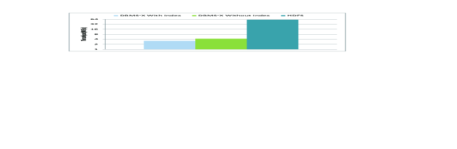
Figure 3: DBMS-X vs HDFS Write Performance

The lower figure in Figure 2 shows the current solution - a Hadoop / Hive and RDBMS-based storage and analysis system. Hadoop / Hive are mainly utilized for data collecting, data analysis and ad-hoc query. The RDBMS is still a good choice for online query and CRUD operations on the archive data. The current solution combines the advantage of off-line batch processing and high write throughput of Hadoop ecosystem with the advantage of powerful OLTP of RDBMS. It releases the burden of RDBMS on big data analysis, and make Hadoop a data collecting / computing engine for the whole system. After system migration, the burden on the RDBMS is much smaller than before. Introducing such an cost-efficient open source platform into Smart Grid is not costly, on the contrary, it will consequently make it possible to reduce the ”heavy armor” configuration of the RDBMS-X, which do not need to raise but significantly reduce the overall budget. The IT team and the financial manager meet in their way to the business objective. Another advantage is that open source Hadoop ecosystem can be customized for Smart Grid, for example, adding dedicated effective multidimensional index - DGFIndex, one of our efforts for improving the performance of Hadoop/Hive on big data analysis of Zhejiang Grid.

In the current solution, meter data is directly written into HDFS by multiple HDFS clients. Although, HBase[4] as an alternative to HDFS could also enable high write throughput and support more update operations than append as does HDFS. Also, Hive could perform queries on HBase. However, based on our experiments using a TPC-H workload, the query performance of Hive on HDFS is 3-4 times better than that of Hive on HBase. To get high analysis performance, we use HDFS directly as the storage of meter data. The archive data is stored in RDBMS, so as to perform efficient CRUD operations by users. Furthermore, a copy of archive data is stored in HDFS, which facilitates join operation analysis between archive data and meter data. The two copies need to be consistent. The analysis results (i.e., statistic data) are written into RDBMS for online query. The SQL statements in stored procedures of the RDBMS are transformed to corresponding HiveQL statements by our mapping tool [26]. The HiveQL statements in a stored procedure are organized as work flow in Oozie [9]. All stored procedures, archive data synchronization, and statistic data ETL are scheduled by the coordinator in Oozie.

Previous experiments questioned the performance of Hadoop/Hive in comparison to RDBMSs or parallel databases [23, 24]. However, many improvements have be developed for Hadoop / Hive [14] and its performance has increased significantly. One of the main reasons leading to poor performance of Hadoop / Hive is that scan-based query processing method. To solve this problem, adding effective index can improves Hadoop/Hive’s performance dramatically [20]. Other Hadoop/Hive optimization for Zhejiang Grid applications we have done are presented in [26, 19]. Furthermore, much data analysis in Zhejiang Grid is based on loops on separate regions, thus the logic can easily be parallelized. However, in current RDBMS, the degree of parallelism is highly limited by the configuration of the number of CPU cores, the memory capacity and the speed of disk I/O. Higher degrees of parallelism will need more high-end servers, which will lead to higher costs. In a Hadoop / Hive cluster, we only need to add cheap commodity servers, which puts less pressure on the budget. With a higher degree of parallelism, efficient indexes, and other optimizations, Hadoop / Hive’s performance can be comparable or even better than that of expensive RDBMSs.

Parallel databases could also be a candidate for data analysis in the State Grid. But it has the same drawbacks with RDBMS, e.g., its write throughput is much lower than HDFS [23, 24]. Again, the software license cost is also high and it requires sophisticated configuration parameter tuning and query performance optimization, and lots of maintenance efforts.

4 DGFIndex

In the following, we will present our novel indexing technique DGFIndex for multidimensional range queries.

4.1 DGFIndex Architecture

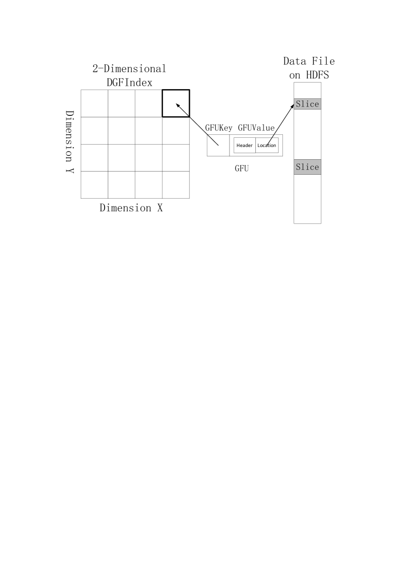
Figure 4: DGFIndex Architecture

Figure 4 shows a 2-dimensional DGFIndex, in which dimension X and Y can be any two dimensions in the record of the meter data. DGFIndex uses a grid file to split the data space into small units named grid file unit (GFU), which consists of GFUKey and GFUValue. GFUKey is defined as the left lower coordinate of each GFU in the data space. GFUValue consists of the header and the location of the data Slice stored in HDFS. A Slice is a segment of a file in HDFS. The header in GFUValue contains pre-computed aggregation values of numerical dimensions, such as max, min, sum, count, and other UDFs (need to be additive functions) supported by Hive. For example, we can pre-compute $sum(num*price)$ of all records located in the same GFU. The location in GFUValue contains the start and end offset of the corresponding Slice. All records in a Slice belong to the same GFU.

An example of a DGFIndex can be seen in Figure 5. In the example, there is a Hive table consisting of three dimensions: A, B, and C. Suppose that the most frequently queried HiveQL statement on this table is like the one shown in Listing 2.

⬇

SELECT SUM(C)

FROM Table

WHERE A>=5 AND A<12

AND B>=12 AND B<16;

Listing 2: Multidimensional Range HiveQL Query

We build DGFIndex for dimensions A and B. Dimension A and B are equally divided into intervals with granularity of 3 and 2, respectively. Every interval is left closed-right open, e.g., $[1,4)$. The data space is divided into GFUs along dimension A and B. The records are scattered in these GFUs. For example, the first record $<1,14,0.1>$ is located in the region $\{(A,B)|1\leq A<4,13\leq B<15\}$. All records in the same GFU are stored in a single HDFS Slice. Every GFU is a key-value pair, for example, the key-value pair of the highlighted GFU is as showed in Figure 5. The GFUKey 7_13 is the left lower coordinate of the red one. The first part in GFUValue is pre-computed sum(C) of all records in the Slice. Users can specify any Hive supported functions and UDFs when constructing an DGFIndex. Once a DGFIndex is deployed, users can still add more UDFs dynamically to DGFIndex on demand. The second part in GFUValue is the location of the Slice on HDFS.

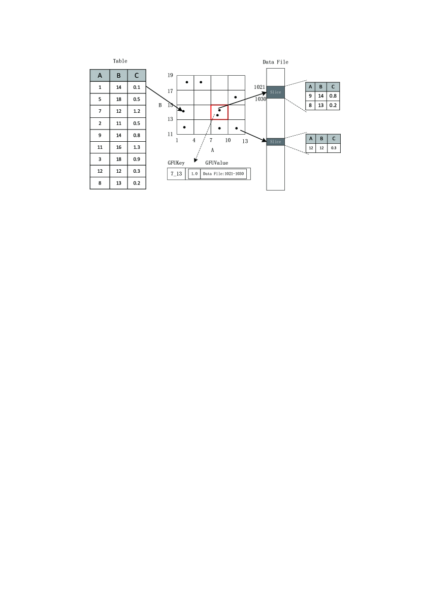
Figure 5: DGFIndex Example

Since the index will become fairly big after many insertions, we can utilize a distributed key-value store, such as HBase, Cassandra, or Voldemort to improve the performance of the index access. In the current implementation, we use HBase as the storage system for DGFIndex.

4.2 DGFIndex Construction

Algorithm 1 Map(Text line)

1:  $idxDValue=\textbf{getIdxDimensionList}(line)$;

2:  $GFUKey=\phi;$

3:  for $value$ in $idxDValue$ do

4:     $GFUKey\bigcup\textbf{standard}(value);$

5:  end for

6:  $\textbf{emit}<GFUKey,line>$

Before constructing a DGFIndex, one needs to specify the splitting policy (the interval size of every index dimension) according to the distribution of the meter data. The construction of DGFIndex is a MapReduce job. The job reorganizes the meter data into a set of Slices based on the specified splitting policy. In the meantime, it builds a GFUKey-GFUValue pair for every Slice and adds the pair into the key-value store. The details of the job is showed in Algorithm 1 and Algorithm 2. In the map phase, the mapper first gets all values of index dimensions (Line 1). Then, the mapper standardizes each value based on the splitting policy and combines these standard values to generate GFUKey (Lines 2-5). The ”standard” method is to find the previous coordinate in splitting policy relative to the value on this dimension. At last, the mapper emits $<GFUKey,line>$ to the reducer. In the reduce phase, the reducer first sets the start and end position of current Slice as the current offset of the output file of reducer and -1 respectively (Line 1-2), and then sets the sliceSize equal to 0, fileName as the current output file’s name, header as null (Line 3-5). Second, the reducer computes all the pre-computed values and combines them into header, the sliceSize records the cumulative size of current Slice (Line 6-12). At last, the reducer computes the end position of current Slice and GFUValue (Line 13-14), then the reducer puts the $<GFUKey,GFUValue>$ pair into the key-value store. In addition, the minimum and maximum standardized values in every index dimensions are stored in the key-value store when constructing a DGFIndex. This information is very useful when the number of index dimension in a query is less than the number of index dimension in the DGFIndex.

Algorithm 2 Reduce(Text GFUKey, List$<$Text$>$ lineList)

1:  $start=current\ offset\ of\ ouput\ file;$

2:  $end=-1;$

3:  $sliceSize=0;$

4:  $fileName=current\ ouput\ file^{\prime}s\ name;$

5:  $header=NULL;$

6:  for $line$ in $lineList$ do

7:     $preComValue=\textbf{getPreComDimensionList}(line)$;

8:     for $value$ in $preComValue$ do

9:        $header=\textbf{combine}(header,\textbf{preCompute}(value));$

10:     end for

11:     $sliceSize=sliceSize+\textbf{sizeOf}(line);$

12:  end for

13:  $end=end+sliceSize$

14:  $GFUValue=<header,<fileName,start,end>>;$

15:  $KVStore.\textbf{put}(GFUKey,GFUValue);$

An example of the DGFIndex construction is shown in Figure 6. The 5th and 9th record are located in the same GFU, thus, after reorganization, the two records are stored together in a Slice. Suppose that the size of every record is 9 bytes. After the index construction, every Slice generates a $<GFUKey,GFUValue>$ pair. In this example, we pre-compute sum(C) from every Slice. From the example, we can see that the maximum number of $<GFUKey,GFUValue>$ pairs is the number of GFU no matter how many distinct value exist in every index dimension.The number of records in index table is fairly small compared with the existing indexes in Hive. For example, if we have a table containing 1000 records, we create Compact Index for 3 dimensions which have 10 distinct value respectively. There will be 1000 records in index table, same with base table. If we create DGFIndex for these 3 dimensions with interval of 2 respectively. There are only 125 records in key-value store.

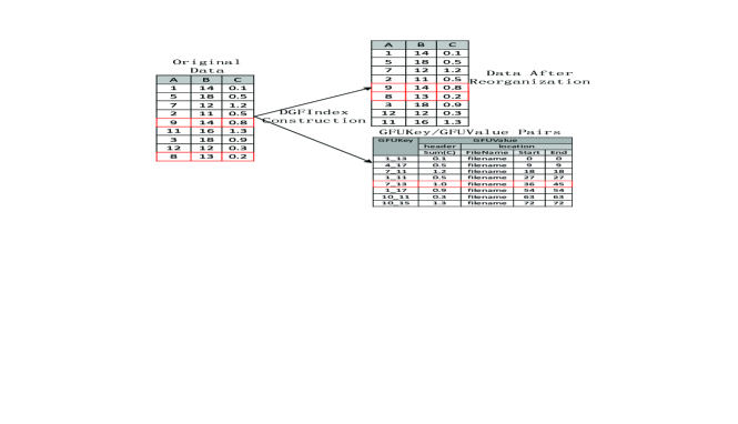
Figure 6: DGFIndex Construct Example

In our implementation, the syntax of constructing an DGFIndex is the same as constructing a Compact Index in Hive except that the user needs to specify the splitting policy and pre-computing UDF in IDXPROPERTIES part as shown in Listing 3. We specify the minimum value and interval for every index dimension. For date type, we also need to specify the unit of interval.

⬇

CREATE INDEX idx_a_b

ON TABLE Table(A,B)

AS ’org...dgf.DgfIndexHandler’

IDXPROPERTIES (’A’=’1_3’, ’B’=’11_2’,

’precompute’=’sum(C)’);

Listing 3: DGFIndex Creation

There is a time stamp field in the meter data and it has been added as a default dimension in our index. When the new meter data flow is written into HDFS, these data first is stored in several temporary files. After these data is verified, the time stamp dimension in DGFIndex is extended and the DGFIndex construction process is executed on these temporary files, and the reorganized data is written into the table directory. Thus, the data load process is the same as the original HDFS, it does not influenced by our index.

4.3 DGFIndex Query

The DGFIndex query process can be divided into three steps. In the first step, as shown in Algorithm 3, when the DGFIndex handler receives a predicate from Hive, it first extracts the related index value from the predicate (Line 1). If the number of index dimension in predicate is less than the number of index dimension in DGFIndex, the DGFIndex handler will get the minimum and maximum standardized value of the missing index dimension from the key-value store. Then the DGFIndex handler gets the query related GFUs based on the splitting policy. There are two kinds of GFUs, one is entirely in the query region (inner GFU) (Line 2), another is partially in query region (boundary GFU) (Line 3). For inner GFUs, if the query is only an aggregation or UDF like query, we only require the header from the key-value store, and do not need to access data from HDFS. Thus, we can easily get the sub result from these headers of the inner GFUs, and write it to a temporary file (Line 5-7). When Hive finishes computing the boundary GFUs, the two sub results are combined, and returned to the user. If the query is not an aggregation or UDF like query, we need to get all locations of the query-related Slices(not scanning the index table which is different with Hive’s indexes) from the key-value store, and write them to a temporary file to help filter unrelated splits (Line 9-12).

Algorithm 3 DGFIndex Query(predicate)

1:  $idxPred=\textbf{extract}(predicate);$

2:  $innerKeySet=DGFIndex.\textbf{search}(idxPred);$

3:  $boundaryKeySet=DGFIndex.\textbf{search}(idxPred);$

4:  $queryKeySet=boundaryKeySet$

5:  if $isAggregationQuery$ then

6:     $subResult=KVStore.\textbf{getHeader}(innerKeySet);$

7:     $\textbf{writeToTmpFile}(subResult);$

8:  else

9:     $queryKeySet=queryKeySet\bigcup innerKeySet;$

10:  end if

11:  $sliceLoc=KVStore.\textbf{getLocation}(queryKeySet);$

12:  $\textbf{writeToTmpFile}(sliceLoc);$

In the second step, as shown in Algorithm 4, the algorithm is implemented in DgfInputFormat.getSplits(). The process is similar to the Compact Index. First, we get the set of Slices from the temporary file in Algorithm 3 (Line 2). Then, we get all splits according to the name of files in the set of Slices (Line 3). The splits that fully contain or overlap with Slices will be chosen (Line 4-8). We prepare a $<split,slicesInSplit>$ pair for every chosen split to filter unrelated Slices in split (Line 9-12). The $sliceInSplit$ is ordered by $start$ offset of every Slice.

Algorithm 4 Split Filter

1:  $chosenSplit=\phi;$

2:  $sliceSet=\textbf{readFromTmpFile}();$

3:  $allSplit=\textbf{getSplitsFromSliceSet}($sliceSet$);$

4:  for $split$ in $allSplit$ do

5:     if $split\bigcap sliceSet\neq\phi$ then

6:        $chosenSplit=chosenSplit\bigcup split$

7:     end if

8:  end for

9:  for $split$ in $chosenSplit$ do

10:     $slicesInSplit=\textbf{getRelatedSlices}(sliceSet);$

11:     $KVStore.put(split,slicesInSplit);$

12:  end for

13:  $return\ chosenSplit;$

In the third step, we implement a $RecordReader$ that can skip unrelated Slices in a split. At the initialization of the $RecordReader$, it gets a Slice list from the key-value store for the split it is processing. When the mapper invokes the $next$ function in the RecordReader, we only need to read the records in each Slice and skip the margin between adjacent Slices.

The processing of the query in Listing 2 is shown in Figure 7. In step 1, the query region is $Q:\{(A,B)|5<=A<12,12<=B<16\}$ (highlighted in green), the inner region is $I:\{(A,B)|7\leq A<10,13\leq B<15\}$ (highlighted in red). Because the GFU is the smallest reading unit for our index, the region that needs to be read is $R:\{(A,B)|4\leq A<13,11\leq B<17\}$. Consequently, the boundary region is $R-I$. As the query is an aggregation query, we can get a sub result from I. Then we get the location information of the Slices from the key-value store by GFUKeys located in boundary region. In step 2, we use the Slice location information to filter splits, then we create a Slice list for every chosen split. In our example, we only have one split, the Slice list means we just need to read these regions in the split $<filename:0>$:[18-18],[63-63] and [72-72]. Other regions can be skipped. In Step 3, we can filter unrelated Slices based on the Slice list in Step 2.

A Slice may stretch across two splits. In this case, we divide the Slice into two parts: one is in previous split, another is in the adjacent split. The two Slices are processed by different mappers. In our implementation, DGFIndex is transparent from the user, Hive will automatically use a DGFIndex when processing MDRQs.

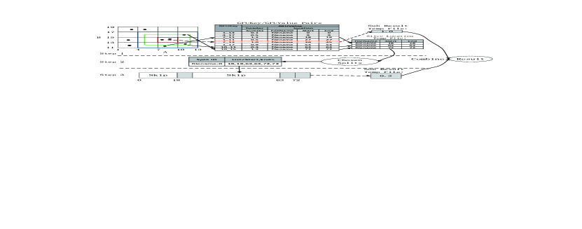
Figure 7: DGFIndex Query Example

5 Experiments and Results

In this section, we evaluate the DGFIndex and compare it with the existing indexes in Hive. Furtermore, we compare DGFIndex with HadoopDB as a comparison with parallel databases [10]. Our experiments mainly focus on three aspects: (1) the size of index, (2) the index construction time, and (3) the query performance.

5.1 Cluster Setup

We conduct experiments on a cluster of 29 virtual nodes. One node is master for Hadoop and HBase, and the remaining 28 nodes are workers. Each node has 8 virtual cores, 8GB memory, and 300GB disk. All nodes run CentOS 6.5, Java 1.6.0_45 64bit, Hadoop-1.2.1 and HBase-0.94.13 as the key-value store. DGFIndex is implemented based on Hive-0.10.0. Every workers in Hadoop is configured with up to 5 mappers and 3 reducers. The replication factor is set to 2 in HDFS. The block size is 64MB default. The mapred.task.io.sort.mb is set 512Mb to achieve better performance. Other configurations in Hadoop, HBase and Hive are default. For HadoopDB, we install it based on the instructions on [3]. We use PostgreSQL 8.4.20 as the storage layer and above Hadoop as the computation layer. Each experiments is run three times and we report the average result.

5.2 DataSet and Query

In our experiments, we use two datasets to verify the efficiency of DGFIndex on processing of MDRQ. The first dataset is the lineitem table from TPC-H ( 4.1 billion, about 518GB in TextFile format, about 468GB in RCFile format, both no compression), we use it as a general case. Another dataset is real world meter data ( 11 billion records, about 1TB in TextFile format, about 890GB in RCFile format, both no compression). This dataset is a kind meter data of a month. The table comprises of 17 fields, which contains userId, regionId( the region where the user lives), the number of how much power consumed, and other metrics, for example positive active total electricity with different rates etc. These fields is not related to our queries in experiments. The number of distinct value in userId, regionId and time is 14 million, 11 and 30 respectively. In real world dataset, the records that have same time are stored together, which is obey the rules of meter data. In addition, the real world data set also contain a user’s information table which is a kind of archive data and is about 2GB. This table will be used to join with meter data table.

We choose some queries from Zhejiang Grid for our experiments, these queries have similar predicate with the SQLs in stored procedures. These chosen queries mainly focus on userId, regionId, and time. The detailed query forms are list in following parts. In each kind of query, we change the selectivity: point query, 5% and 12%. In our experiments, we suppose that there is no partitions in the tables, if there is, we can assume that our data set is in one partition among these partitions.

For HadoopDB, we use its GlobalHasher to partition the meter data into 28 partitions based on the userId. Each node retrieves a 38 GB partition from HDFS. Then we use its LocalHasher to partition the data into 38 chunks based on userId, 1GB each. All chunks are bulk-loaded into separate databases in PostgreSQL. We create a multi-column index on the userId, regionId and time for each meterdata table. The user table is also partitioned into 28 partitions based on userId. Each node retrieves a 83 MB partition and puts it to all the databases of current node. Since the SMS in HadoopDB only supports specific queries, we extend the MapReduce-based query code in HadoopDB to perform the queries in our experiments.

5.3 Real World Data Set

5.3.1 Index Size and Construction Time

For indexes in Hive, we only compare DGFIndex with Compact Index, since Compact index is the basis of Aggregate Index and Bitmap Index. For now, our DGFIndex only supports TextFile table. So we use TextFile table as the base table of DGFIndex. However, it is easy to expend DGFIndex to support other file formats. For the Compact Index, RCFile-based Compact Index will lead to smaller index table size, which will improve the query performance. So, in our experiments, we choose RCFile format table as the base table for the Compact Index.

In an initial experiment, we created a 3-dimensional (userId, regionId, and time) Compact Index for the RCFile table. The size of index table was 821GB, which is almost same with base table. As Hive first scans index table before processing query, the 3-dimensional Compact Index will not improve query performance. So, we only created a 2-dimensional index (regionid and time, which have few distinct values, 11 and 30, respectively). On the other hand, our DGFIndex can easily handle this case. So, we create 3-dimensional DGFIndex in following experiments. Because the number of distinct value in $regionId$ and $time$ is small, we fix the interval size for these: 1 and 1 day respectively. For dimension $userId$, we change the interval size, as follow, to evaluate the influence of different interval size on index size and query performance. (i) Large: split dimension $userId$ equally to 100 intervals with large interval size. (ii) Medium: split dimension $userId$ equally to 1000 intervals with medium interval size. (iii) Small: split dimension $userId$ equally to 10000 intervals with small interval size. What’s more, we pre-compute $sum(powerConsumed)$ when building DGFIndex. This information will be used in Section 5.3.2.

In Table 2, we can see that in the 3-dimensional case, the construction of DGFIndex takes longer time than the construction of the Compact Index, the reason is the base table needs to be reorganized by shuffling all data to reducer via network and pre-computation CPU cost. However, the size of DGFIndex is much smaller than 3-dimensional Compact Index , and almost equal or smaller than 2-dimensional Compact Index. In addition, as the interval size decreases, the number of intervals in $userId$ becomes larger, and the number of GFU also becomes larger, which leads to more $<GFUKey,GFUValue>$ pairs, thus bigger DGFIndex size. In the 2-dimensional case, the size of Compact Index is much smaller than 3-dimensional case. Because the number of distinct value in $regionId$ and $time$ is very small. The combinations of the two dimensions is much smaller than three dimensions. But decreasing the number of index dimensions will decrease the accuracy of index.

Table 2: Index Size and Construction Time

Index	Table	Dimension	Size	Time
Type	Type	Number		(s)
$Compact$	$RCFile$	$3$	$821GB$	$23350$
$Compact$	$RCFile$	$2$	$7MB$	$1884$
$DGF-L$	$TextFile$	$3$	$0.94MB$	$25816$
$DGF-M$	$TextFile$	$3$	$3MB$	$25632$
$DGF-S$	$TextFile$	$3$	$13MB$	$26027$

5.3.2 Aggregation Query

In this part, we will demonstrate the efficiency of pre-computing in DGFIndex. We choose a query like Listing 4. Figure 16, 16, and 16 show the cost time of this query in different selectivities. The upper part of the first two columns in the figures is the time of reading the index and other time(like HiveQL parsing time and launching task time). The lower part is the time of reading the data after filtered by the index and processing. The third column is the cost time of HadoopDB. In HadoopDB, the query in Listing 4 is pushed into all PostgreSQL databases, and then we use a MapReduce job to collect the results. Table 3 shows how many records needed to read after filtered by DGFIndex and Compact Index. We do not show the number for HadoopDB, because it is not easy to get the number out of PostgreSQL after filtering by the index. The $accurate$ in the table means the accurate number of records specified by predicate.

The ScanTable-based time for this kind query is about 1950s. From the result, we can see that Compact Index improves the performance about 26.6, 2.5, 1.7 times over scanning the whole table in different selectivity. In large interval size case, DGFIndex improves the performance about 66.9, 65, 65.5 times over scanning the whole table. In medium interval size case, it improves the performance 67, 59.9, 63.9 times. In small interval size case, it improves the performance 78.1, 54.6, 46.2 times over scaning the whole table. The number of HadoopDB is 32.2, 2.6, 1.3 respectively. What’s more, because of pre-computing, the performance of DGFIndex on aggregation query processing nearly does not be influenced by the query selectivity. HadoopDB has the almost same performance with Compact Index on processing aggregation query. DGFIndex is almost 2-50 times faster than the Compact Index and HadoopDB. We also find that HadoopDB has some performance degradation with the selectivity increasing compared with Compact Index. The reason is that when PostgreSQL processes multiple concurrent queries, it will lead to resources competition, and the low batch reading performance of RDBMS is another reason.

Because we pre-compute $sum(powerConsumed)$ when constructing DGFIndex, Hive only reads the data located in the boundary region. From Table 3, we can see that with the decrease of interval size, the size of $GFU$ also decrease, that is, the accuracy of DGFIndex increases, so Hive needs to read less data. In point query case, there is no inner $GFU$, so Hive needs to read all data located in the $GFU$. Because Compact Index can not filter unrelated data in each splits, Hive will read the whole split, which leads to more data reading.

⬇

SELECT sum(powerConsumed)

FROM meterdata

WHERE regionId>r1 and regionId<r2

and userId>u1 and userId<u2

and time>t1 and time<t2;

Listing 4: Aggregation Query

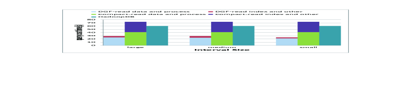
Figure 8: Aggregate Query Time For Point Query

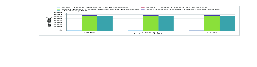
Figure 9: Aggregate Query Time For 5% Selectivity

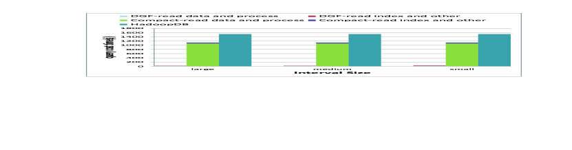
Figure 10: Aggregate Query Time For 12% Selectivity

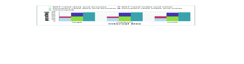
Figure 11: Group By Query Time For Point Query

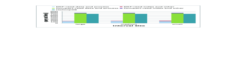
Figure 12: Group By Query Time For 5% Selectivity

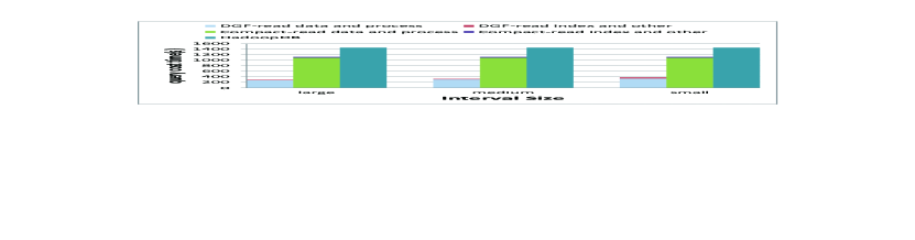
Figure 13: Group By Query Time For 12% Selectivity

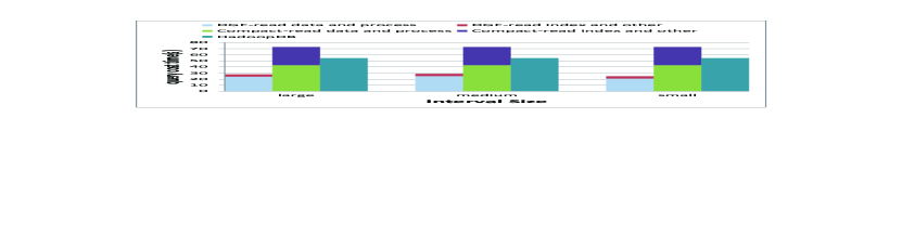
Figure 14: Join Query Time For Point Query

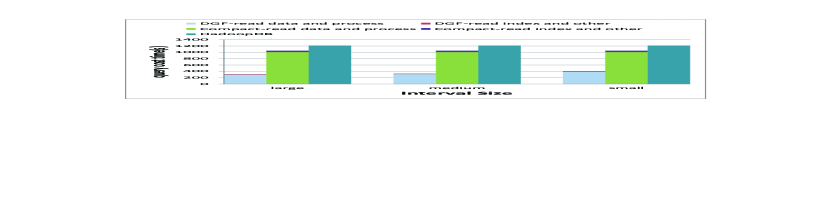
Figure 15: Join Query Time For 5% Selectivity

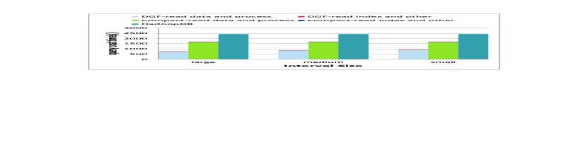
Figure 16: Join Query Time For 12% Selectivity

Table 3: Records Number for Aggregation Query

Index Type	Point	5%	12%
$Compact$	$169,395,953$	$4,756,501,768$	$6,586,886,752$
$DGF-L$	$4,347,200$	$67,678$	$100,386$
$DGF-M$	$4,258,358$	$20,280$	$31,215$
$DGF-S$	$2,291,718$	$16,122$	$23,712$
$Accurate$	$26$	$569,186,384$	$1,354,351,336$

Table 4: Records Number for Group By Query

Index Type	Point	5%	12%
$Compact$	$169,395,953$	$4,756,501,768$	$6,586,886,752$
$DGF-L$	$4,347,200$	$681,321,681$	$1,433,931,728$
$DGF-M$	$4,258,358$	$641,128,331$	$1,401,070,456$
$DGF-S$	$2,291,718$	$572,231,864$	$1,367,754,156$
$Accurate$	$26$	$569,186,384$	$1,354,351,336$

5.3.3 GroupBy Query and Join Query

In this part, we evaluate the performance of DGFIndex on processing non-aggregation query, this means that DGFIndex can not use pre-computed information. We use a Group By query like Listing 5 and a Join query like Listing 6. For HadoopDB, we extend its aggregation task code and join task code to perfom the two queries. The cost time of Group By query is shown in Figure 16,16, 16 and the cost time of Join query is shown in Figure 16, 16, and 16. Table 4 shows the number of records needed to read of Group By query and Join query after they are filtered by the index. The number is same for both query, since their predicate is the same.

In Group By query case, the ScanTable-based time is about 1900s. In Join query case, the time is about 1930s. The Compact Index improves performance 1.2-31 times over scanning the whole table in both cases. HadoopDB improves performance 0.8-35.3 times over scanning the whole table. On other hand, the number of DGFIndex is 2.1-75.8 times. From the result, we can see that DGFIndex is about 2-5 times faster than Compact Index and HadoopDB on different selectivities. From Figure 16,16, we can see that the time of reading index becomes longer with the decreasing of interval size. Because when the interval size becomes smaller, more $GFU$s will be located in query region. The index handler needs to get more GFUValue from HBase. However, storing index in key-value store decreases index reading time. From Figure 16 and 16, we can see that Compact Index and HadoopDB’s performance is almost equal or worse than ScanTable-based style when processing high selectivity query. The reason for Compact Index is the inaccuracy of two dimensional index leads to reading almost all splits. The reason for HadoopDB is resources competition and low batch reading speed. However, for DGFIndex, since it can accurately read related data, thus it can maintain effectiveness for high selectivity query.

As shown in Table 4, as the interval sizes increase, more data is located in one $GFU$. So a DGFIndex with the large interval size needs to read more data than a DGFIndex with small interval size. Which leads to some performance degradation, especially for high selectivity query. However, since DGFIdex can filter unrelated slices when reading each split, the amount of data read by DGFIndex is much smaller than in the case of Compact Index, which improves Hive’s performance dramatically.

⬇

SELECT time,sum(powerConsumed)

FROM meterdata

WHERE regionId>r1 and regionId<r2

and userId>u1 and userId<u2

and time>t1 and time<t2

GROUP BY time;

Listing 5: Aggregation Query

⬇

INSERT OVERWRITE DIRECORY ’/tmp/result’

SELECT t2.userName,t1.powerConsumed

FROM meterdata t1

JOIN userInfo t2

ON t1.userId=t2.userId

WHERE t1.regionId>r1 AND t1.regionId<r2

AND t1.userId>u1 AND t1.userId<u2

AND t1.time>t1 AND t1.time<t2;

Listing 6: Join Query

5.3.4 Partial Specified Query

In practice, the number of dimensions in the predicate clause may be more or less than the indexed dimensions. If the number is more than indexed dimensions, DGFIndex just uses the indexed dimensions in the predicate to filter unrelated data; If the number is less than indexed dimensions, DGFIndex gets the minimum and maximum value of the missing dimension from HBase to complement the predicate. This part evaluates the second case. Because the number of $userId$ values is the largest among the three index dimensions. We delete the $userId$ range condition from predicate, and choose a query as shown in Listing 7. The result is shown in Figure 17. From the result we can see that DGFIndex is 2-4.6 times faster than Compact Index.

⬇

SELECT SUM(powerConsumed)

FROM meterdata

WHERE regionId=11

AND time=’2012-12-30’;

Listing 7: Partital Query

5.4 TPC-H Data Set

In this part, we want to demonstrate the efficiency of DGFIndex for general case, not only for meter data. In this experiment, we use the Q6 in TPC-H as our query. We create 2-dimensional(l_discount and l_quantity, which have few distinct value) and 3-dimensional Compact Index for lineitem table. For DGFIndex, we set the interval size of l_discount, l_quantity and l_shipdate to 0.01, 1.0 and 100 days respectively. The index size and constructing time are showed in Table 5. The query performance is showed in Figure 18. Table 6 shows how many records needed to read after filtered by index.

The ScanTable-based time for this query is 632s. In this case, 2-dimensional and 3-dimensioinal Compact Index both are slower than scanning the whole table. Because Compact Index does not filter any split. DGFIndex is 25 times faster than Compact Index. The index size and the number of data needed read of DGFindex is much smaller than Compact Index. From the result, we can see that the performance of Compact Index is much worse than real world data set. The difference between real world data set and TPC-H data set is that the real world data set actually is sorted by time, however, in TPC-H data set, the records are evenly scattered in data files. Because Compact Index does not reorganize data, it can not improve query performance on this kind of data.

Table 5: Index Size and Construction Time for TPC-H

Index	Table	Dimension	Size	Time
Type	Type	Number		(s)
$Compact$	$RCFile$	$3$	$189GB$	$7367$
$Compact$	$RCFile$	$2$	$637MB$	$991$
$DGFIndex$	$TextFile$	$3$	$4.3MB$	$10997$

Table 6: Records Number for TPC-H Workload

Index Type	Record Number
$Whole\ Table$	$4,095,002,340$
$Compact-3$	$4,095,002,340$
$Compact-2$	$4,095,002,340$
$DGFIndex$	$85,430,966$
$Accurate$	$77,955,077$

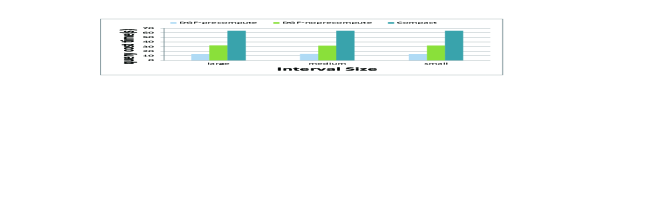
Figure 17: Partial Query Time

Figure 18: TPC-H Workload Query Time

6 Experience About Hive Index

In this section, we will report some findings and some practical experience about performance improvement of Hive at the aspect of index. For now, the existing indexes in Hive are not practical and hard to use, as there is limited documentation and usage examples. Without reading the source code of Hive to get more information about the indexes, they are not usable. The Compact Index is the basis of other indexes. The number of records it stores is decided by the number of combinations of indexed dimensions and the number of data files. The performance of Compact Index is dependent of the size of the index table and the distribution of the values of indexed dimensions. If the index dimensions have few distinct values and the data file of the table is sorted by the indexed dimension, a good query performance improvement can be achieved using Compact Index. On the other hand, if the indexed dimension has many distinct values and they are evenly distributed in the data files, no performance improvement can be achieved with Compact Index. On the contrary, the performance will be worse than scanning the whole table. The idea of the technique of the Aggregate Index is good, but in practice, there are very few use case that can meet its restrictions.

In industry, the most practical method to improve query performance in Hive currently is partition. Partition reorganizes data into different directories based on partition dimension. The best way to improve Hive performance is combining partition with Compact Index. However, the user need to make sure that the index dimensions do not have too many distinct value and are not evenly distributed.

7 Related Work

As mentioned above, the existing indexes in Hive, Compact Index, Bitmap Index and Aggregate Index, are closely related to our DGFIndex. However, they are not well fitted to process multidimensional range queries. [10] combines MapReduce and RDBMS, and uses the indexes in RDBMS to filter unrelated data in every worker. But the data loading speed is lower than HDFS, and its multiple databases storage mode easily leads to serious resource competition, especially for high selectivity query.

Current various parallel databases have been applied for many companies, such as Greenplum, Teradata, Aster Data, Netezza, Datallegro, Dataupia, Vertica, ParAccel, Neoview, DB2(via the Database Partitioning Feature), and Oracle(via Exadata). But these systems have low data loading performance and the software license is very expensive. What’s more, they usually need complex configuration parameters tuning and lots of maintenance efforts[23]. Our objective in this paper is to provide a scalable and cost effective solution for the big meter data problem in Zhejiang Grid, the solution’s performance can be comparable or even better than parallel database, but with much low budget.

In the context of index on HDFS, [20] proposes a kind of one-dimensional range index for sorted file on HDFS. The sorted file is divided into some equal-size pages. It creates one index entry which comprises of the start, end value and offset for every page. [13] proposes two kinds of indexes, Trojan index and Trojan join index, to filter unrelated splits and improve the performance of join tasks respectively. In Trojan index, it stores the first key, last key and records number for every split. [16] stores the range information for every numerical and date field dimensions in a split, and creates a inverted index for the string type dimension. Since these values are rarely changing, it create a materialized view to store them in a separate file. [21] creates LZO block level full-text inverted index for data on HDFS to accelerate selection operations that contains free-text filters. Both, [20] and [13] mainly focus on one-dimensional index and they need to sort data file based on index dimension. The primary purpose of [20], [13], and [16] is filtering unrelated splits. They can not filter unrelated records in a split. [21] can not process multidimensional range query. In contrast, DGFIndex can process multidimensional query efficiently, and does not need to sort data files based on index dimensions. It only puts these records in the same GFU together in a file. Moreover, DGFIndex can filter unrelated Slices in a split.

In the context of spatial database on Hadoop, Spatial Hadoop[15] proposes a two level multidimensional index on Hadoop. It first partitions data using Grid File, R-Tree or R+-Tree into equal-size block(64MB), second creates local index for each block, the local index is stored as a file on HDFS, third it create global index for all block, the global index is stored in master’s memory. Spatial Hadoop is mainly for spatial data types, such as Point, Rectangle and Polygon. Hadoop-Gis[11] also proposes a two level spatial index on Hadoop. It splits data with grid partition into small size tiles, which is much smaller than 64MB. Then a global index is created to stored the MBRs of these tiles, it is stored in the memory of master. The local index of each tile is created on demand based on the query type. Both indexes are applied in spatial applications, which is much different with our index, our DGFIndex is for improving the traditional applications. Another difference is that our DGFIndex is organized as one level index, which is simpler and easier to maintenance than the both above. The last difference is that we combine pre-aggregated technique with Grid File, which makes aggregation query processing more effective.

8 Conclusion and Future Work

In this paper, we share the system migration experience from traditional RDBMS to Hadoop based system. To improve Hadoop/Hive’s performance on smart meter big data analysis, we propose a multidimensional range index named DGFIndex. By dividing the data space into some $GFU$s, DGFIndex only stores the information of $GFU$ rather than the combinations of index dimensions. This method reduces the index size dramatically. With $GFU$-based pre-computing, DGFIndex enhances greatly the multidimensional aggregation processing ability of Hive. DGFIndex first filters splits with $Slice$ location information, then skips unrelated $Slice$ in each split. By doing this, DGFIndex reduces greatly the number of data need to read and improve the performance of Hive. Our experiments on real world data set and TPC-H data set demonstrate that DGFIndex not only improve the performance of Hive on meter data, but also is applicable to general data set. In future work, we will work on an algorithm to find the best splitting policy for DGFIndex based on the distribution of the meter data and the query history. The optimal placement of $Slice$s will also be our next step research problem.

Acknowledgements: This work is supported by the National Natural Science Foundation of China under Grant No.61070027, 61020106002, 61161160566. This work is also supported by Technology Project of the State Grid Corporation of China under Grant No.SG [2012] 815.

References

- [1] Cloudera blog. https://blog.cloudera.com/blog/2009/02/the-small-files-problem/.
- [2] Hadoop. http://hadoop.apache.org/.
- [3] Hadoopdb install instructions. http://hadoopdb.sourceforge.net/guide/.
- [4] Hbase. https://hbase.apache.org/.
- [5] Hive. http://hive.apache.org/.
- [6] Hive aggregate index. https://issues.apache.org/jira/browse/HIVE-1694.
- [7] Hive bitmap index. https://issues.apache.org/jira/browse/HIVE-1803.
- [8] Hive compact index. https://issues.apache.org/jira/browse/HIVE-417.
- [9] Oozie. https://oozie.apache.org/.
- [10] A. Abouzeid, K. Bajda-Pawlikowski, D. Abadi, A. Silberschatz, and A. Rasin. Hadoopdb: an architectural hybrid of mapreduce and dbms technologies for analytical workloads. Proceedings of the VLDB Endowment, 2(1):922–933, 2009.
- [11] A. Aji, F. Wang, H. Vo, R. Lee, Q. Liu, X. Zhang, and J. Saltz. Hadoop gis: a high performance spatial data warehousing system over mapreduce. Proceedings of the VLDB Endowment, 6(11):1009–1020, 2013.
- [12] J. Dean and S. Ghemawat. Mapreduce: Simplified data processing on large clusters. Communications of the ACM, 51(1):107–113, 2008.
- [13] J. Dittrich, J.-A. Quiané-Ruiz, A. Jindal, Y. Kargin, V. Setty, and J. Schad. Hadoop++: Making a yellow elephant run like a cheetah (without it even noticing). Proceedings of the VLDB Endowment, 3(1-2):515–529, 2010.
- [14] C. Doulkeridis and K. Nørvåg. A survey of large-scale analytical query processing in mapreduce. The VLDB Journal, pages 1–26, 2013.
- [15] A. Eldawy and M. F. Mokbel. A demonstration of spatialhadoop: an efficient mapreduce framework for spatial data. Proceedings of the VLDB Endowment, 6(12):1230–1233, 2013.
- [16] M. Y. Eltabakh, F. Özcan, Y. Sismanis, P. J. Haas, H. Pirahesh, and J. Vondrak. Eagle-eyed elephant: split-oriented indexing in hadoop. In Proceedings of the 16th International Conference on Extending Database Technology, pages 89–100. ACM, 2013.
- [17] S. Ghemawat, H. Gobioff, and S.-T. Leung. The google file system. In SOSP ’03: Proceedings of the 19th ACM Symposium on Operating Systems Principles, pages 29–43, 2003.
- [18] Y. He, R. Lee, Y. Huai, Z. Shao, N. Jain, X. Zhang, and Z. Xu. Rcfile: A fast and space-efficient data placement structure in mapreduce-based warehouse systems. In Data Engineering (ICDE), 2011 IEEE 27th International Conference on, pages 1199–1208. IEEE, 2011.
- [19] S. Hu, W. Liu, T. Rabl, S. Huang, Y. Liang, Z. Xiao, H.-A. Jacobsen, and X. Pei. Dualtable: A hybrid storage model for update optimization in hive. CoRR, abs/1404.6878, 2014.
- [20] D. Jiang, B. C. Ooi, L. Shi, and S. Wu. The performance of mapreduce: An in-depth study. Proceedings of the VLDB Endowment, 3(1-2):472–483, 2010.
- [21] J. Lin, D. Ryaboy, and K. Weil. Full-text indexing for optimizing selection operations in large-scale data analytics. In Proceedings of the second international workshop on MapReduce and its applications, pages 59–66. ACM, 2011.
- [22] J. Nievergelt, H. Hinterberger, and K. C. Sevcik. The grid file: An adaptable, symmetric multikey file structure. ACM Transactions on Database Systems (TODS), 9(1):38–71, 1984.
- [23] A. Pavlo, E. Paulson, A. Rasin, D. J. Abadi, D. J. DeWitt, S. Madden, and M. Stonebraker. A comparison of approaches to large-scale data analysis. In Proceedings of the 2009 ACM SIGMOD International Conference on Management of data, pages 165–178. ACM, 2009.
- [24] M. Stonebraker, D. Abadi, D. J. DeWitt, S. Madden, E. Paulson, A. Pavlo, and A. Rasin. Mapreduce and parallel dbmss: friends or foes? Communications of the ACM, 53(1):64–71, 2010.
- [25] A. Thusoo, J. S. Sarma, N. Jain, Z. Shao, P. Chakka, N. Zhang, S. Antony, H. Liu, and R. Murthy. Hive-a petabyte scale data warehouse using hadoop. In Data Engineering (ICDE), 2010 IEEE 26th International Conference on, pages 996–1005. IEEE, 2010.
- [26] Y. Xu and S. Hu. Qmapper: a tool for sql optimization on hive using query rewriting. In Proceedings of the 22nd international conference on World Wide Web companion, pages 211–212. International World Wide Web Conferences Steering Committee, 2013.