EUROPEAN ORGANIZATION FOR NUCLEAR RESEARCH (CERN)
![]() CERN-PH-EP-2014-069
LHCb-PAPER-2014-012
22 April 2014
CERN-PH-EP-2014-069
LHCb-PAPER-2014-012
22 April 2014
Measurement of the resonant and components in decays
The LHCb collaboration†††Authors are listed on the following pages.
The resonant structure of the reaction is studied using data from 3 of integrated luminosity collected by the LHCb experiment, one-third at 7 center-of-mass energy and the remainder at 8. The invariant mass of the pair and three decay angular distributions are used to determine the fractions of the resonant and non-resonant components. Six interfering states: , , , , and are required to give a good description of invariant mass spectra and decay angular distributions. The positive and negative fractions of each of the resonant final states are determined. The meson is not seen and the upper limit on its presence, compared with the observed rate, is inconsistent with a model where these scalar mesons are formed from two quarks and two anti-quarks (tetraquarks) at the eight standard deviation level. In the model, the absolute value of the mixing angle between the and the scalar mesons is limited to be less than at 90% confidence level.
Submitted to Phys. Rev. D
© CERN on behalf of the LHCb collaboration, license CC-BY-3.0.
LHCb collaboration
R. Aaij41,
B. Adeva37,
M. Adinolfi46,
A. Affolder52,
Z. Ajaltouni5,
J. Albrecht9,
F. Alessio38,
M. Alexander51,
S. Ali41,
G. Alkhazov30,
P. Alvarez Cartelle37,
A.A. Alves Jr25,38,
S. Amato2,
S. Amerio22,
Y. Amhis7,
L. An3,
L. Anderlini17,g,
J. Anderson40,
R. Andreassen57,
M. Andreotti16,f,
J.E. Andrews58,
R.B. Appleby54,
O. Aquines Gutierrez10,
F. Archilli38,
A. Artamonov35,
M. Artuso59,
E. Aslanides6,
G. Auriemma25,n,
M. Baalouch5,
S. Bachmann11,
J.J. Back48,
A. Badalov36,
V. Balagura31,
W. Baldini16,
R.J. Barlow54,
C. Barschel38,
S. Barsuk7,
W. Barter47,
V. Batozskaya28,
Th. Bauer41,
A. Bay39,
L. Beaucourt4,
J. Beddow51,
F. Bedeschi23,
I. Bediaga1,
S. Belogurov31,
K. Belous35,
I. Belyaev31,
E. Ben-Haim8,
G. Bencivenni18,
S. Benson50,
J. Benton46,
A. Berezhnoy32,
R. Bernet40,
M.-O. Bettler47,
M. van Beuzekom41,
A. Bien11,
S. Bifani45,
T. Bird54,
A. Bizzeti17,i,
P.M. Bjørnstad54,
T. Blake48,
F. Blanc39,
J. Blouw10,
S. Blusk59,
V. Bocci25,
A. Bondar34,
N. Bondar30,38,
W. Bonivento15,38,
S. Borghi54,
A. Borgia59,
M. Borsato7,
T.J.V. Bowcock52,
E. Bowen40,
C. Bozzi16,
T. Brambach9,
J. van den Brand42,
J. Bressieux39,
D. Brett54,
M. Britsch10,
T. Britton59,
N.H. Brook46,
H. Brown52,
A. Bursche40,
G. Busetto22,q,
J. Buytaert38,
S. Cadeddu15,
R. Calabrese16,f,
M. Calvi20,k,
M. Calvo Gomez36,o,
A. Camboni36,
P. Campana18,38,
D. Campora Perez38,
A. Carbone14,d,
G. Carboni24,l,
R. Cardinale19,38,j,
A. Cardini15,
H. Carranza-Mejia50,
L. Carson50,
K. Carvalho Akiba2,
G. Casse52,
L. Cassina20,
L. Castillo Garcia38,
M. Cattaneo38,
Ch. Cauet9,
R. Cenci58,
M. Charles8,
Ph. Charpentier38,
S.-F. Cheung55,
N. Chiapolini40,
M. Chrzaszcz40,26,
K. Ciba38,
X. Cid Vidal38,
G. Ciezarek53,
P.E.L. Clarke50,
M. Clemencic38,
H.V. Cliff47,
J. Closier38,
V. Coco38,
J. Cogan6,
E. Cogneras5,
P. Collins38,
A. Comerma-Montells11,
A. Contu15,38,
A. Cook46,
M. Coombes46,
S. Coquereau8,
G. Corti38,
M. Corvo16,f,
I. Counts56,
B. Couturier38,
G.A. Cowan50,
D.C. Craik48,
M. Cruz Torres60,
S. Cunliffe53,
R. Currie50,
C. D’Ambrosio38,
J. Dalseno46,
P. David8,
P.N.Y. David41,
A. Davis57,
K. De Bruyn41,
S. De Capua54,
M. De Cian11,
J.M. De Miranda1,
L. De Paula2,
W. De Silva57,
P. De Simone18,
D. Decamp4,
M. Deckenhoff9,
L. Del Buono8,
N. Déléage4,
D. Derkach55,
O. Deschamps5,
F. Dettori42,
A. Di Canto38,
H. Dijkstra38,
S. Donleavy52,
F. Dordei11,
M. Dorigo39,
A. Dosil Suárez37,
D. Dossett48,
A. Dovbnya43,
F. Dupertuis39,
P. Durante38,
R. Dzhelyadin35,
A. Dziurda26,
A. Dzyuba30,
S. Easo49,38,
U. Egede53,
V. Egorychev31,
S. Eidelman34,
S. Eisenhardt50,
U. Eitschberger9,
R. Ekelhof9,
L. Eklund51,38,
I. El Rifai5,
Ch. Elsasser40,
S. Ely59,
S. Esen11,
T. Evans55,
A. Falabella16,f,
C. Färber11,
C. Farinelli41,
N. Farley45,
S. Farry52,
D. Ferguson50,
V. Fernandez Albor37,
F. Ferreira Rodrigues1,
M. Ferro-Luzzi38,
S. Filippov33,
M. Fiore16,f,
M. Fiorini16,f,
M. Firlej27,
C. Fitzpatrick38,
T. Fiutowski27,
M. Fontana10,
F. Fontanelli19,j,
R. Forty38,
O. Francisco2,
M. Frank38,
C. Frei38,
M. Frosini17,38,g,
J. Fu21,38,
E. Furfaro24,l,
A. Gallas Torreira37,
D. Galli14,d,
S. Gallorini22,
S. Gambetta19,j,
M. Gandelman2,
P. Gandini59,
Y. Gao3,
J. Garofoli59,
J. Garra Tico47,
L. Garrido36,
C. Gaspar38,
R. Gauld55,
L. Gavardi9,
E. Gersabeck11,
M. Gersabeck54,
T. Gershon48,
Ph. Ghez4,
A. Gianelle22,
S. Giani’39,
V. Gibson47,
L. Giubega29,
V.V. Gligorov38,
C. Göbel60,
D. Golubkov31,
A. Golutvin53,31,38,
A. Gomes1,a,
H. Gordon38,
C. Gotti20,
M. Grabalosa Gándara5,
R. Graciani Diaz36,
L.A. Granado Cardoso38,
E. Graugés36,
G. Graziani17,
A. Grecu29,
E. Greening55,
S. Gregson47,
P. Griffith45,
L. Grillo11,
O. Grünberg62,
B. Gui59,
E. Gushchin33,
Yu. Guz35,38,
T. Gys38,
C. Hadjivasiliou59,
G. Haefeli39,
C. Haen38,
S.C. Haines47,
S. Hall53,
B. Hamilton58,
T. Hampson46,
X. Han11,
S. Hansmann-Menzemer11,
N. Harnew55,
S.T. Harnew46,
J. Harrison54,
T. Hartmann62,
J. He38,
T. Head38,
V. Heijne41,
K. Hennessy52,
P. Henrard5,
L. Henry8,
J.A. Hernando Morata37,
E. van Herwijnen38,
M. Heß62,
A. Hicheur1,
D. Hill55,
M. Hoballah5,
C. Hombach54,
W. Hulsbergen41,
P. Hunt55,
N. Hussain55,
D. Hutchcroft52,
D. Hynds51,
M. Idzik27,
P. Ilten56,
R. Jacobsson38,
A. Jaeger11,
J. Jalocha55,
E. Jans41,
P. Jaton39,
A. Jawahery58,
M. Jezabek26,
F. Jing3,
M. John55,
D. Johnson55,
C.R. Jones47,
C. Joram38,
B. Jost38,
N. Jurik59,
M. Kaballo9,
S. Kandybei43,
W. Kanso6,
M. Karacson38,
T.M. Karbach38,
M. Kelsey59,
I.R. Kenyon45,
T. Ketel42,
B. Khanji20,
C. Khurewathanakul39,
S. Klaver54,
O. Kochebina7,
M. Kolpin11,
I. Komarov39,
R.F. Koopman42,
P. Koppenburg41,38,
M. Korolev32,
A. Kozlinskiy41,
L. Kravchuk33,
K. Kreplin11,
M. Kreps48,
G. Krocker11,
P. Krokovny34,
F. Kruse9,
M. Kucharczyk20,26,38,k,
V. Kudryavtsev34,
K. Kurek28,
T. Kvaratskheliya31,
V.N. La Thi39,
D. Lacarrere38,
G. Lafferty54,
A. Lai15,
D. Lambert50,
R.W. Lambert42,
E. Lanciotti38,
G. Lanfranchi18,
C. Langenbruch38,
B. Langhans38,
T. Latham48,
C. Lazzeroni45,
R. Le Gac6,
J. van Leerdam41,
J.-P. Lees4,
R. Lefèvre5,
A. Leflat32,
J. Lefrançois7,
S. Leo23,
O. Leroy6,
T. Lesiak26,
B. Leverington11,
Y. Li3,
M. Liles52,
R. Lindner38,
C. Linn38,
F. Lionetto40,
B. Liu15,
G. Liu38,
S. Lohn38,
I. Longstaff51,
J.H. Lopes2,
N. Lopez-March39,
P. Lowdon40,
H. Lu3,
D. Lucchesi22,q,
H. Luo50,
A. Lupato22,
E. Luppi16,f,
O. Lupton55,
F. Machefert7,
I.V. Machikhiliyan31,
F. Maciuc29,
O. Maev30,
S. Malde55,
G. Manca15,e,
G. Mancinelli6,
M. Manzali16,f,
J. Maratas5,
J.F. Marchand4,
U. Marconi14,
C. Marin Benito36,
P. Marino23,s,
R. Märki39,
J. Marks11,
G. Martellotti25,
A. Martens8,
A. Martín Sánchez7,
M. Martinelli41,
D. Martinez Santos42,
F. Martinez Vidal64,
D. Martins Tostes2,
A. Massafferri1,
R. Matev38,
Z. Mathe38,
C. Matteuzzi20,
A. Mazurov16,f,
M. McCann53,
J. McCarthy45,
A. McNab54,
R. McNulty12,
B. McSkelly52,
B. Meadows57,55,
F. Meier9,
M. Meissner11,
M. Merk41,
D.A. Milanes8,
M.-N. Minard4,
N. Moggi14,
J. Molina Rodriguez60,
S. Monteil5,
D. Moran54,
M. Morandin22,
P. Morawski26,
A. Mordà6,
M.J. Morello23,s,
J. Moron27,
R. Mountain59,
F. Muheim50,
K. Müller40,
R. Muresan29,
M. Mussini14,
B. Muster39,
P. Naik46,
T. Nakada39,
R. Nandakumar49,
I. Nasteva2,
M. Needham50,
N. Neri21,
S. Neubert38,
N. Neufeld38,
M. Neuner11,
A.D. Nguyen39,
T.D. Nguyen39,
C. Nguyen-Mau39,p,
M. Nicol7,
V. Niess5,
R. Niet9,
N. Nikitin32,
T. Nikodem11,
A. Novoselov35,
A. Oblakowska-Mucha27,
V. Obraztsov35,
S. Oggero41,
S. Ogilvy51,
O. Okhrimenko44,
R. Oldeman15,e,
G. Onderwater65,
M. Orlandea29,
J.M. Otalora Goicochea2,
P. Owen53,
A. Oyanguren64,
B.K. Pal59,
A. Palano13,c,
F. Palombo21,t,
M. Palutan18,
J. Panman38,
A. Papanestis49,38,
M. Pappagallo51,
C. Parkes54,
C.J. Parkinson9,
G. Passaleva17,
G.D. Patel52,
M. Patel53,
C. Patrignani19,j,
A. Pazos Alvarez37,
A. Pearce54,
A. Pellegrino41,
M. Pepe Altarelli38,
S. Perazzini14,d,
E. Perez Trigo37,
P. Perret5,
M. Perrin-Terrin6,
L. Pescatore45,
E. Pesen66,
K. Petridis53,
A. Petrolini19,j,
E. Picatoste Olloqui36,
B. Pietrzyk4,
T. Pilař48,
D. Pinci25,
A. Pistone19,
S. Playfer50,
M. Plo Casasus37,
F. Polci8,
A. Poluektov48,34,
E. Polycarpo2,
A. Popov35,
D. Popov10,
B. Popovici29,
C. Potterat2,
A. Powell55,
J. Prisciandaro39,
A. Pritchard52,
C. Prouve46,
V. Pugatch44,
A. Puig Navarro39,
G. Punzi23,r,
W. Qian4,
B. Rachwal26,
J.H. Rademacker46,
B. Rakotomiaramanana39,
M. Rama18,
M.S. Rangel2,
I. Raniuk43,
N. Rauschmayr38,
G. Raven42,
S. Reichert54,
M.M. Reid48,
A.C. dos Reis1,
S. Ricciardi49,
A. Richards53,
M. Rihl38,
K. Rinnert52,
V. Rives Molina36,
D.A. Roa Romero5,
P. Robbe7,
A.B. Rodrigues1,
E. Rodrigues54,
P. Rodriguez Perez54,
S. Roiser38,
V. Romanovsky35,
A. Romero Vidal37,
M. Rotondo22,
J. Rouvinet39,
T. Ruf38,
F. Ruffini23,
H. Ruiz36,
P. Ruiz Valls64,
G. Sabatino25,l,
J.J. Saborido Silva37,
N. Sagidova30,
P. Sail51,
B. Saitta15,e,
V. Salustino Guimaraes2,
C. Sanchez Mayordomo64,
B. Sanmartin Sedes37,
R. Santacesaria25,
C. Santamarina Rios37,
E. Santovetti24,l,
M. Sapunov6,
A. Sarti18,m,
C. Satriano25,n,
A. Satta24,
M. Savrie16,f,
D. Savrina31,32,
M. Schiller42,
H. Schindler38,
M. Schlupp9,
M. Schmelling10,
B. Schmidt38,
O. Schneider39,
A. Schopper38,
M.-H. Schune7,
R. Schwemmer38,
B. Sciascia18,
A. Sciubba25,
M. Seco37,
A. Semennikov31,
K. Senderowska27,
I. Sepp53,
N. Serra40,
J. Serrano6,
L. Sestini22,
P. Seyfert11,
M. Shapkin35,
I. Shapoval16,43,f,
Y. Shcheglov30,
T. Shears52,
L. Shekhtman34,
V. Shevchenko63,
A. Shires9,
R. Silva Coutinho48,
G. Simi22,
M. Sirendi47,
N. Skidmore46,
T. Skwarnicki59,
N.A. Smith52,
E. Smith55,49,
E. Smith53,
J. Smith47,
M. Smith54,
H. Snoek41,
M.D. Sokoloff57,
F.J.P. Soler51,
F. Soomro39,
D. Souza46,
B. Souza De Paula2,
B. Spaan9,
A. Sparkes50,
F. Spinella23,
P. Spradlin51,
F. Stagni38,
S. Stahl11,
O. Steinkamp40,
O. Stenyakin35,
S. Stevenson55,
S. Stoica29,
S. Stone59,
B. Storaci40,
S. Stracka23,38,
M. Straticiuc29,
U. Straumann40,
R. Stroili22,
V.K. Subbiah38,
L. Sun57,
W. Sutcliffe53,
K. Swientek27,
S. Swientek9,
V. Syropoulos42,
M. Szczekowski28,
P. Szczypka39,38,
D. Szilard2,
T. Szumlak27,
S. T’Jampens4,
M. Teklishyn7,
G. Tellarini16,f,
F. Teubert38,
C. Thomas55,
E. Thomas38,
J. van Tilburg41,
V. Tisserand4,
M. Tobin39,
S. Tolk42,
L. Tomassetti16,f,
D. Tonelli38,
S. Topp-Joergensen55,
N. Torr55,
E. Tournefier4,
S. Tourneur39,
M.T. Tran39,
M. Tresch40,
A. Tsaregorodtsev6,
P. Tsopelas41,
N. Tuning41,
M. Ubeda Garcia38,
A. Ukleja28,
A. Ustyuzhanin63,
U. Uwer11,
V. Vagnoni14,
G. Valenti14,
A. Vallier7,
R. Vazquez Gomez18,
P. Vazquez Regueiro37,
C. Vázquez Sierra37,
S. Vecchi16,
J.J. Velthuis46,
M. Veltri17,h,
G. Veneziano39,
M. Vesterinen11,
B. Viaud7,
D. Vieira2,
M. Vieites Diaz37,
X. Vilasis-Cardona36,o,
A. Vollhardt40,
D. Volyanskyy10,
D. Voong46,
A. Vorobyev30,
V. Vorobyev34,
C. Voß62,
H. Voss10,
J.A. de Vries41,
R. Waldi62,
C. Wallace48,
R. Wallace12,
J. Walsh23,
S. Wandernoth11,
J. Wang59,
D.R. Ward47,
N.K. Watson45,
D. Websdale53,
M. Whitehead48,
J. Wicht38,
D. Wiedner11,
G. Wilkinson55,
M.P. Williams45,
M. Williams56,
F.F. Wilson49,
J. Wimberley58,
J. Wishahi9,
W. Wislicki28,
M. Witek26,
G. Wormser7,
S.A. Wotton47,
S. Wright47,
S. Wu3,
K. Wyllie38,
Y. Xie61,
Z. Xing59,
Z. Xu39,
Z. Yang3,
X. Yuan3,
O. Yushchenko35,
M. Zangoli14,
M. Zavertyaev10,b,
F. Zhang3,
L. Zhang59,
W.C. Zhang12,
Y. Zhang3,
A. Zhelezov11,
A. Zhokhov31,
L. Zhong3,
A. Zvyagin38.
1Centro Brasileiro de Pesquisas Físicas (CBPF), Rio de Janeiro, Brazil
2Universidade Federal do Rio de Janeiro (UFRJ), Rio de Janeiro, Brazil
3Center for High Energy Physics, Tsinghua University, Beijing, China
4LAPP, Université de Savoie, CNRS/IN2P3, Annecy-Le-Vieux, France
5Clermont Université, Université Blaise Pascal, CNRS/IN2P3, LPC, Clermont-Ferrand, France
6CPPM, Aix-Marseille Université, CNRS/IN2P3, Marseille, France
7LAL, Université Paris-Sud, CNRS/IN2P3, Orsay, France
8LPNHE, Université Pierre et Marie Curie, Université Paris Diderot, CNRS/IN2P3, Paris, France
9Fakultät Physik, Technische Universität Dortmund, Dortmund, Germany
10Max-Planck-Institut für Kernphysik (MPIK), Heidelberg, Germany
11Physikalisches Institut, Ruprecht-Karls-Universität Heidelberg, Heidelberg, Germany
12School of Physics, University College Dublin, Dublin, Ireland
13Sezione INFN di Bari, Bari, Italy
14Sezione INFN di Bologna, Bologna, Italy
15Sezione INFN di Cagliari, Cagliari, Italy
16Sezione INFN di Ferrara, Ferrara, Italy
17Sezione INFN di Firenze, Firenze, Italy
18Laboratori Nazionali dell’INFN di Frascati, Frascati, Italy
19Sezione INFN di Genova, Genova, Italy
20Sezione INFN di Milano Bicocca, Milano, Italy
21Sezione INFN di Milano, Milano, Italy
22Sezione INFN di Padova, Padova, Italy
23Sezione INFN di Pisa, Pisa, Italy
24Sezione INFN di Roma Tor Vergata, Roma, Italy
25Sezione INFN di Roma La Sapienza, Roma, Italy
26Henryk Niewodniczanski Institute of Nuclear Physics Polish Academy of Sciences, Kraków, Poland
27AGH - University of Science and Technology, Faculty of Physics and Applied Computer Science, Kraków, Poland
28National Center for Nuclear Research (NCBJ), Warsaw, Poland
29Horia Hulubei National Institute of Physics and Nuclear Engineering, Bucharest-Magurele, Romania
30Petersburg Nuclear Physics Institute (PNPI), Gatchina, Russia
31Institute of Theoretical and Experimental Physics (ITEP), Moscow, Russia
32Institute of Nuclear Physics, Moscow State University (SINP MSU), Moscow, Russia
33Institute for Nuclear Research of the Russian Academy of Sciences (INR RAN), Moscow, Russia
34Budker Institute of Nuclear Physics (SB RAS) and Novosibirsk State University, Novosibirsk, Russia
35Institute for High Energy Physics (IHEP), Protvino, Russia
36Universitat de Barcelona, Barcelona, Spain
37Universidad de Santiago de Compostela, Santiago de Compostela, Spain
38European Organization for Nuclear Research (CERN), Geneva, Switzerland
39Ecole Polytechnique Fédérale de Lausanne (EPFL), Lausanne, Switzerland
40Physik-Institut, Universität Zürich, Zürich, Switzerland
41Nikhef National Institute for Subatomic Physics, Amsterdam, The Netherlands
42Nikhef National Institute for Subatomic Physics and VU University Amsterdam, Amsterdam, The Netherlands
43NSC Kharkiv Institute of Physics and Technology (NSC KIPT), Kharkiv, Ukraine
44Institute for Nuclear Research of the National Academy of Sciences (KINR), Kyiv, Ukraine
45University of Birmingham, Birmingham, United Kingdom
46H.H. Wills Physics Laboratory, University of Bristol, Bristol, United Kingdom
47Cavendish Laboratory, University of Cambridge, Cambridge, United Kingdom
48Department of Physics, University of Warwick, Coventry, United Kingdom
49STFC Rutherford Appleton Laboratory, Didcot, United Kingdom
50School of Physics and Astronomy, University of Edinburgh, Edinburgh, United Kingdom
51School of Physics and Astronomy, University of Glasgow, Glasgow, United Kingdom
52Oliver Lodge Laboratory, University of Liverpool, Liverpool, United Kingdom
53Imperial College London, London, United Kingdom
54School of Physics and Astronomy, University of Manchester, Manchester, United Kingdom
55Department of Physics, University of Oxford, Oxford, United Kingdom
56Massachusetts Institute of Technology, Cambridge, MA, United States
57University of Cincinnati, Cincinnati, OH, United States
58University of Maryland, College Park, MD, United States
59Syracuse University, Syracuse, NY, United States
60Pontifícia Universidade Católica do Rio de Janeiro (PUC-Rio), Rio de Janeiro, Brazil, associated to2
61Institute of Particle Physics, Central China Normal University, Wuhan, Hubei, China, associated to3
62Institut für Physik, Universität Rostock, Rostock, Germany, associated to11
63National Research Centre Kurchatov Institute, Moscow, Russia, associated to31
64Instituto de Fisica Corpuscular (IFIC), Universitat de Valencia-CSIC, Valencia, Spain, associated to36
65KVI - University of Groningen, Groningen, The Netherlands, associated to41
66CBU-Manisa, Manisa, Turkey, associated to38
aUniversidade Federal do Triângulo Mineiro (UFTM), Uberaba-MG, Brazil
bP.N. Lebedev Physical Institute, Russian Academy of Science (LPI RAS), Moscow, Russia
cUniversità di Bari, Bari, Italy
dUniversità di Bologna, Bologna, Italy
eUniversità di Cagliari, Cagliari, Italy
fUniversità di Ferrara, Ferrara, Italy
gUniversità di Firenze, Firenze, Italy
hUniversità di Urbino, Urbino, Italy
iUniversità di Modena e Reggio Emilia, Modena, Italy
jUniversità di Genova, Genova, Italy
kUniversità di Milano Bicocca, Milano, Italy
lUniversità di Roma Tor Vergata, Roma, Italy
mUniversità di Roma La Sapienza, Roma, Italy
nUniversità della Basilicata, Potenza, Italy
oLIFAELS, La Salle, Universitat Ramon Llull, Barcelona, Spain
pHanoi University of Science, Hanoi, Viet Nam
qUniversità di Padova, Padova, Italy
rUniversità di Pisa, Pisa, Italy
sScuola Normale Superiore, Pisa, Italy
tUniversità degli Studi di Milano, Milano, Italy
1 Introduction
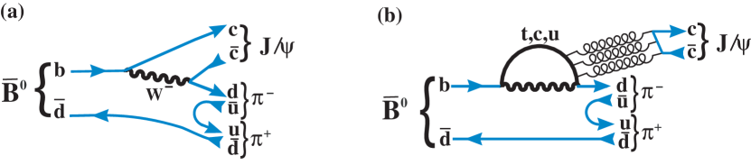
The decay mode is of particular interest in the study of violation in the system.111In this paper, mention of a particular decay mode implies the use of the charge conjugate decay as well, unless stated otherwise. The decay can proceed either via a tree level process, shown in Fig. 1(a), or via the penguin mechanisms shown in Fig. 1(b). The ratio of penguin to tree amplitudes is enhanced in this decay relative to [1, *Faller:2008zc]. Thus the effects of penguin topologies can be investigated by using the decay and comparing different measurements of the violating phase, , in , and individual channels such as .
The decay is also useful for the study of the substructure of light mesons that decay into . Tests have been proposed to ascertain if the scalar and mesons are formed of or tetraquarks. In the model of Ref. [3], if these scalar states are tetraquarks, the ratio of decay widths is predicted to be 1/2. If instead these are states, they can be mixtures of two base states; in this scenario the width ratio can be any value and is determined principally by the mixing angle between the base states.
The decay was first observed by the BaBar collaboration [Aubert:2002vb, *Aubert:2007xw]. It has been previously studied by LHCb using data from 1 of integrated luminosity [5]. The branching fraction was measured to be . The mass and angular distributions were used to measure the resonant substructure. That analysis, however, did not use the angle between the and decay planes, due to limited statistics. A new theoretical approach [6] now allows us to include all the angular information and measure the fraction of -even and -odd states. This information is vital to any subsequent violation measurements.
2 Data sample and detector
In this paper, we measure the resonant substructure and content of the decay from data corresponding to 3 of integrated luminosity collected with the LHCb detector [7] using collisions. One-third of the data was acquired at a center-of-mass energy of 7, and the remainder at 8. The detector is a single-arm forward spectrometer covering the pseudorapidity range , designed for the study of particles containing or quarks. The detector includes a high-precision tracking system consisting of a silicon-strip vertex detector surrounding the interaction region, a large-area silicon-strip detector located upstream of a dipole magnet with a bending power of about , and three stations of silicon-strip detectors and straw drift tubes [8] placed downstream. The combined tracking system provides a momentum measurement with relative uncertainty that varies from 0.4% at 5 to 0.6% at 100,222We work in units where . and impact parameter (IP) resolution of 20 for tracks with large transverse momentum (). Different types of charged hadrons are distinguished by information from two ring-imaging Cherenkov (RICH) detectors[9]. Photon, electron and hadron candidates are identified by a calorimeter system consisting of scintillating-pad and preshower detectors, an electromagnetic calorimeter and a hadronic calorimeter. Muons are identified by a system composed of alternating layers of iron and multiwire proportional chambers [10].
The trigger consists of a hardware stage, based on information from the calorimeter and muon systems, followed by a software stage that applies a full event reconstruction [11]. Events selected for this analysis are triggered by a decay, where the meson is required at the software level to be consistent with coming from the decay of a meson by use either of IP requirements or detachment of the meson decay vertex from the primary vertex (PV). In the simulation, collisions are generated using Pythia [12, *Sjostrand:2007gs] with a specific LHCb configuration [14]. Decays of hadronic particles are described by EvtGen [15], in which final state radiation is generated using Photos [16]. The interaction of the generated particles with the detector and its response are implemented using the Geant4 toolkit [17, 18] as described in Ref. [19].
3 Decay amplitude formalism
3.1 Observables used in the analysis
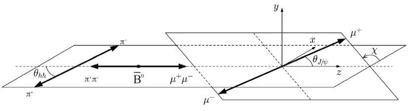
The decay with can be described by the invariant mass of the () pair, and three angles: (i) the angle between the direction in the rest frame with respect to the direction in the rest frame, ; (ii) the angle between the direction and the opposite direction of the candidate momentum in the rest frame, ; and (iii) the angle between the and decay planes in the rest frame, . The angular variables are illustrated in Fig. 2.
In our previous study [5], we used the “Dalitz-plot” variables: the invariant mass squared of , , and the invariant mass squared of the pair, . Due to the spin, the event distributions in the and plane do not directly show the effect of the matrix-element squared. Since the probability density functions (PDFs) expressed as functions of and are easier to normalize, we use them instead. In this paper, the notation is equivalent to . The Dalitz-plot variables can be translated into (, ), and vice versa. The formalism described below is for the decay sequence , .
3.2 Amplitude formalism
The decay rate of has been described in detail in Ref. [6]. The differential decay width can be written in terms of the decay time and the four other variables and as [20, *Bigi:2000yz]
| (1) |
| (2) |
where is a constant; is the amplitude of at the decay time , which is itself a function of and , summed over all resonant (and possibly non-resonant) components; is the mass difference between the heavy and light mass eigenstates, and the width difference;333We use the conventions that and , where and correspond to the light and heavy mass eigenstates, respectively. and are complex parameters that describe the relation between mass and flavor eigenstates. In this analysis we take to be equal to unity.
Forming the sum of and decay widths and integrating over decay time, yields the time-integrated and flavor-averaged decay width
| (3) |
where we drop the term arising from quantum interference of the amplitudes in the last line. This results from the fact that the factor is negligibly small for meson decays. Specifically,
| (4) |
where is the decay time dependent detection efficiency.444For uniform acceptance, . Since is of the order of for meson decays [22], the term is about the same size.
We define to be the mass line shape of the resonance , which in most cases is a Breit-Wigner function. It is combined with the decay properties of the and resonance to form the expression for the decay amplitude. For each resonance :
| (5) |
Here () is the scalar momentum of one of the two daughters of the resonance (or the meson) in the (or ) rest frame, is the spin of , is the orbital angular momentum between the and system, and the orbital angular momentum in the decay, and thus is the same as the spin of the resonance. and are the centrifugal barrier factors for the and the resonance, respectively [23]. The factor results from converting the phase space of the Dalitz-plot variables and to that of and . The function defined in Eq. (5) is based on previous amplitude analyses [24, 23].
We must sum over all final states, , so for each helicity, denoted by , equal to , and we have the overall decay amplitudes:
| (6) |
where the Wigner- functions are defined in Ref. [22] and are complex helicity coefficients. We note that the value of the is equal to that of the resonance. Finally, the total decay rate of at is given by
| (7) |
In order to determine the components, it is convenient to replace the complex helicity coefficients by the complex transversity coefficients using the relations
| (8) |
Here corresponds to the longitudinal polarization of the meson, and the other two coefficients correspond to polarizations of the meson and system transverse to the decay axis: for parallel polarization of the and , and for perpendicular polarization.
Assuming the absence of direct violation, the relation between the and transversity coefficients is , where is the eigenvalue of the transversity component for the intermediate state , and denotes the or components. Note that for the system both and are given by , so the of the system is always even. The total of the final state is , since the of the is also even. The final state parities, for S, P, and D-waves, are listed in Table 1.
In this analysis a fit determines the amplitude modulus and the phase of the amplitude
| (9) |
for each resonance , and each transversity component . For the amplitude, the value of spin-1 (or spin-2) resonances is 1 (or 2). While the other transversity components, 0 or , have two possible values of 0 and 2 (or 1 and 3) for spin-1 (or -2) resonances. We use only the smaller values for each. Studies show that our results for fractions of different interfering components are not sensitive to these choices.
| Spin | |||
|---|---|---|---|
| 0 | |||
| 1 | 1 | 1 | |
| 2 | 1 |
3.3 Dalitz fit fractions
A complete description of the decay is given in terms of the fitted complex amplitudes. Knowledge of the contribution of each component can be summarized by defining a fit fraction for each transversity , . To determine one needs to integrate over all the four variables: . The interference terms between different helicity components vanish after integrating Eq. (3.2) over the two variables of and , i.e.
| (10) |
The decay rate is the sum of the contributions from the three helicity terms. To define the transversity fractions, we need to write Eq. (3.3) in terms of transversity amplitudes. Since , the sum of the three helicity terms is equal to the sum of three transversities, given as
| (11) |
Thus, we define the transversity fit fractions as
| (12) |
where for , and for or .
The sum of the fit fractions is not necessarily unity due to the potential presence of interference between two resonances. Interference term fractions are given by
| (13) |
and
| (14) |
Interference between different spin- states vanishes when integrated over angle, because the angular functions are orthogonal.
4 Selection requirements
In this analysis we adopt a two step selection. The first step, preselection, is followed by a multivariate selection based on a boosted decision tree (BDT) [25]. Preselection criteria are implemented to preserve a large fraction of the signal events, yet reject easily eliminated backgrounds, and are identical to those used in Ref. [5]. A candidate is reconstructed by combining a candidate with two pions of opposite charge. To ensure good track reconstruction, each of the four particles in the candidate is required to have the track fit /ndf to be less than 4, where ndf is the number of degrees of freedom of the fit. The candidate is formed by two identified muons of opposite charge having greater than 500 , and with a geometrical fit vertex less than 16. Only candidates with dimuon invariant mass between and from the observed mass peak are selected, and are then constrained to the mass [22] for subsequent use.
Each pion candidate is required to have greater than 250 , and that the scalar sum, is required to be larger than 900 . Both pions must have greater than 9 to reject particles produced from the PV. The is computed as the difference between the of the PV reconstructed with and without the considered track. Both pions must also come from a common vertex with , and form a vertex with the with a /ndf less than 10 (here ndf equals five). Pion candidates are identified using the RICH and muon systems. The particle identification makes use of the logarithm of the likelihood ratio comparing two particle hypotheses (DLL). For the pion selection we require DLL and DLL. The candidate must have a flight distance of more than 1.5 . The angle between the combined momentum vector of the decay products and the vector formed from the positions of the PV and the decay vertex (pointing angle) is required to be less than .
The BDT uses eight variables that are chosen to provide separation between signal and background. These are the minimum of DLL() of the and , , the minimum of of the and , and the properties of vertex , pointing angle, flight distance, and . The BDT is trained on a simulated sample of two million signal events generated uniformly in phase space with unpolarized decays, and a background data sample from the sideband . Then the BDT is tested on independent samples from the same sources. The BDT can take any value from -1 to 1. The distributions of signal and background are approximately Gaussian shaped with r.m.s. of about 0.13. Signal peaks at BDT of 0.27 and background at -0.22. To minimize possible bias on the signal acceptance due to the BDT, we choose a loose requirement of BDT, which has about a signal efficiency and a background rejection rate.
5 Fit model
We first select events based on their invariant mass and then perform a full fit to the decay variables. The invariant mass of the selected combinations is shown in Fig. 3. There is a large peak at the mass and a smaller one at the mass on top of the background. A double Crystal Ball function with common means models the radiative tails and is used to fit each of the signals [26]. The known mass difference [22] is used to constrain the difference in mean values. Other components in the fit model take into account background contributions from and decays combined with a random , with , with , and reflections, and combinatorial backgrounds. The exponential combinatorial background shape is taken from like-sign combinations, that are the sum of and candidates, and found to be a good description in previous studies [23, 27].
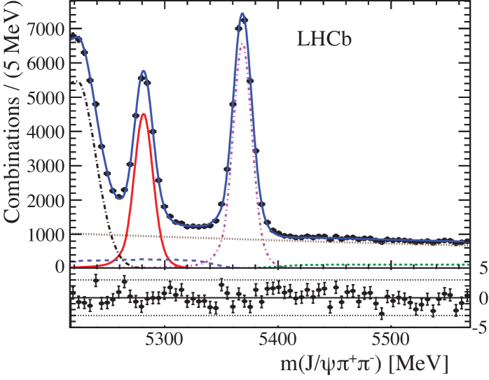
The shapes of the other components are taken from the Monte Carlo simulation with their normalizations allowed to vary. The mass fit gives signal and background candidates within MeV of the mass peak. Only candidates within of the mass peak are retained for further analysis. To improve the resolution of the mass and angular variables used in the amplitude analysis, we perform a kinematic fit constraining the and masses to their PDG mass values [22], and recompute the final state momenta [28].
One of the main challenges in performing a mass and angular analysis is to construct a realistic probability density function, where both the kinematic and dynamical properties are modeled accurately. The PDF is given by the sum of signal, , and background, , functions. The signal includes events from the reaction . These are described by a separate term in the PDF. The total PDF is
| (15) | |||||
where is the fraction of the signal in the fitted region ( obtained from the mass fit in Fig. 3), is the detection efficiency described in Sec. 5.1, and is the background PDF described in Sec. 5.2. The component is modeled by a Gaussian function, , with mean and width . The Gaussian parameters together with the fraction in the peak, , are determined in the fit. The normalization factors for the signal and for the candidates are efficiency-multiplied theoretical functions integrated over the four analysis variables, , , , and , given by
| (16) |
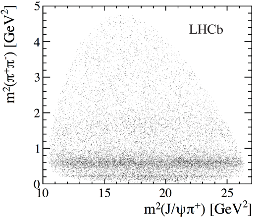
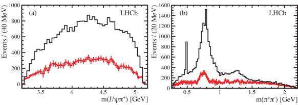
Examination of the event distribution for versus in Fig. 4 shows obvious structures in . To investigate if there are visible exotic structures in , we examine the invariant mass distribution as shown in Fig. 5(a) where we fit the distribution to extract the background levels in bins of (red points). Similarly, Fig. 5(b) shows the mass distribution. Apart from a large signal peak due to the , there are visible structures at about 1270 MeV and a component at about 500 MeV.
5.1 Detection efficiency
The detection efficiency is determined from a sample of about four million simulated events that are generated uniformly in phase space with unpolarized decays. The efficiency model can be expressed as
| (17) |
where and are functions of ; such parameter transformations in are implemented in order to use the Dalitz-plot based efficiency model developed in previous publications [23, 5].
The efficiency dependence on is modeled by
| (18) |
where and . The free parameters are determined by fitting the simulated distributions using Eq. (18) in bins of . The fit gives and GeV-2; , GeV-2 and GeV-4.
The acceptance in depends on . We disentangle this correlation by fitting the distribution in 24 bins of using the parameterization
| (19) |
The fitted values of are modeled by a second order polynomial function
| (20) |
with , GeV-2 and GeV-4.
We model the detection efficiency, , by using the symmetric observables
| (21) |
These variables are related to by
| (22) |
Thus, can be modeled by a two-dimensional fifth order polynomial function as
| (23) | |||||
where all the are the fit parameters. The is 313/299. The values of the parameters are given in Table 2.
| 0.12200.0097 | |
| 0.11630.0182 | |
| 0.00510.0004 | |
| 0.03990.0101 | |
| -0.00120.0007 | |
| 0.100510.0023 | |
| 0.00020.0005 | |
| -0.0001500.000007 | |
| -0.0000110.000261 | |
| 0.0003500.000146 | |
| -0.0001130.000011 |
The projections of the fit used to measure the efficiency parameters are shown in Fig. 6. The efficiency shapes are well described by the parametrization.
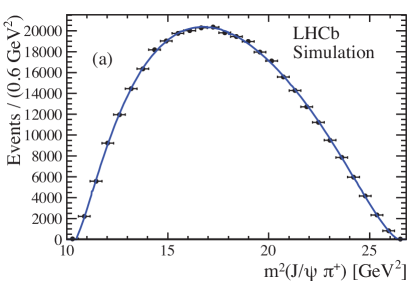
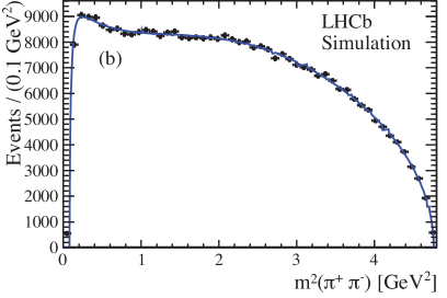
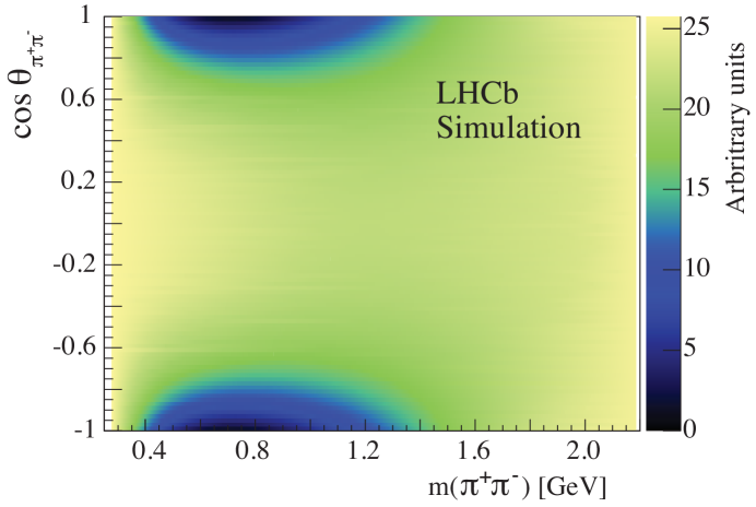
The parameterized efficiency as a function of versus is shown in Fig. 7.
5.2 Background composition
The main background source in the signal region is combinatorial and can be taken from the like-sign combinations within MeV of the mass peak. In addition, there is background arising from partially reconstructed decays (, with and with ), reflections from misidentified and decays, which cannot be present in the like-sign combinations. We use simulated samples of these decays to model their contributions. The normalizations are determined from a previous analysis [29]. The background level in the opposite-sign combination () is studied by fitting the distributions in bins of . The resulting background distribution in the MeV signal region is shown in Fig. 8 by points with error bars. A fit to this distribution gives a partially reconstructed background fraction of 10.7%, the reflection from of 5.3%, and the reflection from the baryon of 15.5% of the total background. The like-sign combinations summed with the additional backgrounds modeled by simulation are shown in Fig. 8.
When this data-simulation hybrid sample is used to extract the background parameters, a further re-weighting procedure is applied based on comparison of distributions between the overall fit and the background data points in Fig. 5(b).

To better model the angular distributions in the mass region, the background is separated into the reflection from , the , and other backgrounds. The total background PDF is sum of these three components:
| (24) |
where the ’s are normalizations, the contributing fractions having values of and ; the other background is normalized as .
The background is modeled by the function
| (25) |
where , , , , are free parameters determined by fitting to the simulation. The last part is a function of the angle. We have verified that the three backgrounds have consistent distributions, thus the parameters and are determined by fitting all backgrounds simultaneously.
The background is described by the function
| (26) |
where , are free parameters. The parameters are obtained by fitting to simulated events.
The model for the remaining backgrounds is
| (27) |
with the function
| (28) |
Here the variable , where and are the fit boundaries, is a fifth order Chebychev polynomial with coefficients (-5), and and are two first order Chebychev polynomials with parameters (-4).
Figure 9 shows the projections of and from the like-sign data combinations added with all the additional simulated backgrounds. The other background includes the background and the combinatorial background which is described by the like-sign combinations. The fitted background parameters are given in Table 3. The background distribution is shown in Fig. 10. Lastly, the background distribution, shown in Fig. 11 fit with the function , determines the parameters and .

| GeV4 | ||||
5.3 Resonance models
| Resonance | Spin | Helicity | Resonance | Mass (MeV) | Width (MeV) | Source |
|---|---|---|---|---|---|---|
| formalism | ||||||
| 1 | BW | PDG [22] | ||||
| 0 | 0 | BW | CLEO [30] | |||
| 2 | BW | PDG [22] | ||||
| 1 | BW | PDG [22] | ||||
| 0 | 0 | Flatté | See text | |||
| 1 | BW | PDG [22] | ||||
| 1 | BW | PDG [22] | ||||
| 0 | 0 | BW | LHCb [31] | |||
| 0 | 0 | BW | PDG [22] |
To study the resonant structures of the decay we use 29 047 event candidates with invariant mass within MeV of the mass peak which include background candidates. The background yield is fixed in the fit. Apart from non-resonant (NR) decays, the possible resonance candidates in the decay are listed in Table 4. We use Breit-Wigner (BW) functions for most of the resonances except . The masses and widths of the BW resonances are listed in Table 4. When used in the fit, they are fixed to these values except for the parameters of which are allowed to vary by their uncertainties. For the we use a Flatté shape [32]. Besides the mass, this shape has two additional parameters and , which are fixed in the fit to the ones obtained from an amplitude analysis of [31], where a large signal is evident. These parameters are MeV, MeV and . All background and efficiency parameters are fixed in the fit.
To determine the complex amplitudes in a specific model, the data are fitted maximizing the unbinned likelihood given as
| (29) |
where is the total number of candidates, and is the total PDF defined in Eq. (15).
6 Fit results
6.1 Final state composition
In order to compare the different models quantitatively, an estimate of the goodness of fit is calculated from 4D partitions of the fitting variables. To distinguish between models, we use the Poisson likelihood [33] defined as
| (30) |
where is the number of events in the four-dimensional bin and is the expected number of events in that bin according to the fitted likelihood function. The and the negative of the logarithm of the likelihood, , of the fits are given in Table 5 for various fitting models, where ndf, the number of degrees of freedom, is equal to minus the number of fit parameters minus one. Here the five-resonance model (5R) contains the resonances: , , , and , the “Best Model” adds a resonance to the 5R model, the 7R model adds a resonance to the Best Model, and the 7R+NR model adds a non-resonant component. We also give the change of for various fits with respect to the 5R model in Table 5.
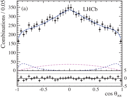
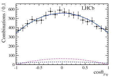
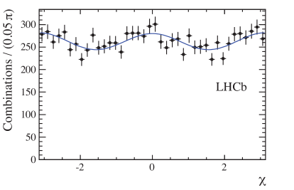
The 7R model gives a slightly better likelihood compared to the Best Model, however, the decrease of the due to adding is less than the expected at 3 significance. Thus, we use the Best Model, which maintains a significance larger than 3 for each resonance component, as our baseline fit, while the 7R model is only used to establish an upper limit on the presence of the . The Dalitz fit projections on the four observables: , , and are shown in Fig. 12 for the Best Model.
| Resonance model | Decrease of | ||
|---|---|---|---|
| 5R Model | 169271 | 2396/2041 | |
| 5R Model + (Best Model) | 169327 | 2293/2035 | |
| Best Model + (7R Model) | 169329 | 2295/2033 | |
| 7R + | 169333 | 2293/2031 | |
| 7R + | 169329 | 2295/2031 | |
| 7R + NR | 169342 | 2292/2031 |

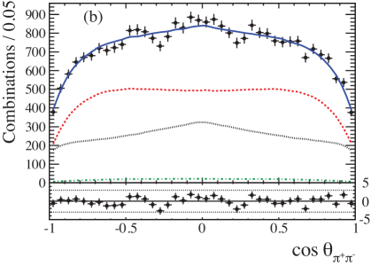
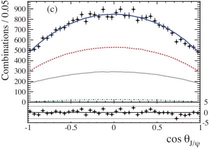
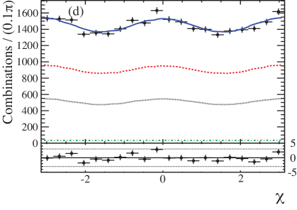
Table 6 shows the summary of fit fractions of different components for various models. The fit fractions of the interference terms in the Best Model are computed using Eq. (13) and listed in Table 7. Table 8 shows the resonant phases from the Best Model. In the Best Model the -even components sum to (56.01.4)%, including the interference terms, so that the -odd fraction is (44.01.4)%. The structure near the peak of the is due to interference. The fit fraction ratio is found to be
where the uncertainties are statistical and systematic, respectively; wherever two uncertainties are quoted in this paper, they will be of this form. The systematic uncertainties will be discussed in detail in Sec. 6.3.
The 7R model fit gives the ratio of observed decays into for equal to . To determine the statistical uncertainty, the full error matrix and parameter values from the fit are used to generate 500 data-size sample parameter sets. For each set, the fit fractions are calculated. The distributions of the obtained fit fractions are described by bifurcated Gaussian functions. The widths of the Gaussians are taken as the statistical errors on the corresponding parameters. We will discuss the implications of this measurement in Sec. 7.
| 5R | Best Model | 7R | 7R+ | 7R+ | 7R+NR | |
| – | – | |||||
| – | – | – | – | – | ||
| – | – | – | – | – | ||
| – | ||||||
| – | ||||||
| – | ||||||
| NR | – | – | – | – | – | |
| Sum | 99.8 | 110.2 | 108.8 | 105.9 | 109.3 | 115.5 |
| Interfering components | Intererence fraction (%) | ||
|---|---|---|---|
| Components | phase (∘) |
|---|---|
| 0 (fixed) | |
| 0 (fixed) | |
In Fig. 13 we show the fit fractions of the different resonant components in the Best Model.
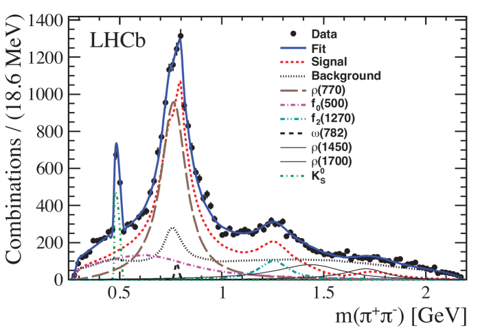
Table 9 lists the fit fractions and the transversity fractions of each contributing resonance. For a - or -wave resonance, we report its total fit fraction by summing all the three components.
| Transversity fractions (%) | ||||
|---|---|---|---|---|
| Component | Fit fraction (%) | |||
| 1 | 0 | 0 | ||
| | ||||
Table 10 shows the branching fractions of the resonant modes calculated by multiplying the fit fraction listed in Table 9 with , obtained from our previous study [5], where the uncertainties are statistical, systematic, and due to normalization, respectively. These branching fractions are proportional to the squares of the individual resonant amplitudes.
6.2 Angular moments
Angular moments are defined as an average of the spherical harmonics, , in each efficiency-corrected and background-subtracted invariant mass interval. The moment distributions provide an additional way of visualizing the effects of different resonances and their interferences, similar to a partial wave analysis. Figure 14 shows the distributions of the angular moments for the Best Model. In general the interpretation of these moments is that is the efficiency corrected and background subtracted event distribution, the sum of the interference between S-wave and P-wave and between P-wave and D-wave amplitudes, the sum of the P-wave, D-wave and the interference of S-wave and D-wave amplitudes, the interference between P-wave and D-wave, the D-wave, and results from an F-wave [23, 34]. For the moments with odd-, one will always find that and have opposite sign; thus the sum of their contributions is expected to be small.

6.3 Systematic uncertainties
The sources of systematic uncertainties on the results of the amplitude analysis are summarized in Table 11. Uncertainties due to particle identification and tracking are taken from Ref. [5] and are taken into account in the branching fraction results, but do not appear in the fit fractions as they are independent of pion kinematics. For the uncertainties due to the acceptance or background modeling, we repeat the data fit 100 times where the parameters of acceptance or background modeling are varied according to the corresponding error matrix. For the acceptance function, the error matrix is obtained by fitting the simulated acceptance as described in Sec. 5.1. For the background function, the error matrix is obtained by fitting the hybrid data-simulated sample as described in Sec. 5.2.
There is uncertainty on the fractions of sources in the hybrid MC-data sample for background modeling. Instead of using the fits to the mass distribution to determine the background fractions, we use the fractions found from the mass fit shown in Fig. 3 that finds the reflection is , the reflection is , the background is and the combinatorial part is , instead of the ones found in Sec. 5.2. We then fit the new hybrid sample to get the background parameters. The data fit is repeated with the new background parameters; the changes on the fit results are added in quadrature with the uncertainties of the background modeling discussed above. The two background uncertainties have similar sizes.
We neglect the mass resolution in the fit where the typical resolution is 3. A previous study shows that the resolution effects are negligible except for the resonance whose total fit fraction is underestimated by . We take the quadrature of 0.09% and 0.08%, equal to 0.12%, as the systematic uncertainty of the total fit fraction of the . These uncertainties are included in the “Acceptance” category.
The uncertainties due to the fit model include adding each resonance that is listed in Table 4 but not used in the 7R model, varying the centrifugal barrier factors defined in Eq. (5) substantially, replacing model by a Bugg function [35] and using the alternative Gounaris and Sakurai Model [36] for the various mesons. The largest variation among those changes is assigned as the systematic uncertainty for modeling. We also find that increasing the default angular momentum for the P and D-wave cases gives negligible differences.
Finally, we repeat the amplitude fit by varying the mass and width of all the resonances except for the , in the 7R model within their errors one at a time, and add the changes in quadrature. For the resonance, we change the resonance parameters , and to the values obtained from Solution II in [31] instead of using the ones obtained from Solution I.
| Item | Acceptance | Background | Fit model | Resonance | Total |
|---|---|---|---|---|---|
| model | parameters | ||||
| Fit fractions (%) | |||||
| Transversity fractions (%) | |||||
| Transversity fractions (%) | |||||
| Transversity fractions (%) | |||||
| Ratio of fit fractions (%) | |||||
7 Substructure of the and mesons
The substructure of mesons belonging to the scalar nonet is controversial. Most mesons are thought to be formed from a combination of a and a . Some authors introduce the concept of states or superpositions of the tetraquark state with the state [37]. In either case, the and the are thought to be mixtures of the underlying states whose mixing angle has been estimated previously. In the model, the mixing is parameterized by a normal 22 rotation matrix characterized by the angle , so that the observed states are given in terms of the base states as
| (31) |
In this case only the part of the wave function contributes (see Fig. 1). Thus we have
| (32) |
where the ’s are phase space factors [3, 38, 37]. The phase space in this pseudoscalar to vector-pseudoscalar decay is proportional to the cube of the momenta. Taking the average of the momentum dependent phase space over the resonant line shapes results in the ratio of phase space factors .
The 7R model fit gives the ratio of branching fractions
We need to correct for the individual branching fractions of the resonances decaying into . BaBar measures the relative branching ratios of of using and decays [39]. BES has extracted relative branching ratios using decays where the , and either both ’s decay into or one into and the other into . Their results [40, *Ablikim:2005kp] are that the relative branching ratio of is [42]. Averaging the two measurements gives
| (33) |
Assuming that the and decays are dominant we can also extract
| (34) |
where we have assumed that the only other decays are to (one-half of the rate), and to neutral kaons (equal to charged kaons). We use , which follows from isospin Clebsch-Gordan coefficients, and assuming that the only decays are into two pions. Since we have only an upper limit on the final state, we will only find an upper limit on the mixing angle, so if any other decay modes of the exist, they would make the limit more stringent.
In order to set an upper limit on , we simulate the final measurement using as input the central value of the measured ratio, the full statistical error matrix obtained from the 7R model fit, and asymmetric Gaussian random variables different for the positive, +3.3%, and negative, %, systematic uncertainties (see Table 11). The resulting rate ratios of to are then multiplied by a factor of where a Gaussian random variable is used for to take into account the uncertainty in the measurement shown in Eq. (34). The upper limit at 90% confidence level is determined when 10% of the simulations exceed the limit value. We find
which translates into a limit of
where we neglect the effect caused by the small systematic uncertainty on the ratio of phase space factors.
If the scalar meson substructure is tetraquark, the wave functions are:
| (35) | |||||
| (36) |
The ratio was predicted to be for pure tetraquark states in Ref. [3]. The measured upper limit on of 0.098 at 90% CL deviates from the tetraquark prediction by 8 standard deviations.
8 Conclusions
We have studied the resonance structure of decays using a modified amplitude analysis. The decay distributions are formed by a series of final states described by individual interfering decay amplitudes. The data are best described by adding coherently the , , , , and resonances, with the largest component being the . The final state is % -even, where we have taken into account both the fit fractions and the interference terms of the different components. Our understanding of the final state composition allows future measurements of violation in these resonant final states. These results supersede those obtained in Ref. [5].
There is no evidence for resonance production. We limit the absolute value of the mixing angle between the lightest two scalar states, the and the , in the model to be less than an absolute value of at 90% confidence level. We find that production is much smaller than predicted for tetraquarks, which we rule out at the 8 standard deviation level using the model of Ref. [3]. Concern has been expressed [37] that if the were a tetraquark state the measurement of the mixing-dependent -violating phase in the decay could be affected due to additional decay mechanisms. Our result here alleviates this potential source of error.
Acknowledgements
We express our gratitude to our colleagues in the CERN accelerator departments for the excellent performance of the LHC. We thank the technical and administrative staff at the LHCb institutes. We acknowledge support from CERN and from the national agencies: CAPES, CNPq, FAPERJ and FINEP (Brazil); NSFC (China); CNRS/IN2P3 and Region Auvergne (France); BMBF, DFG, HGF and MPG (Germany); SFI (Ireland); INFN (Italy); FOM and NWO (The Netherlands); SCSR (Poland); MEN/IFA (Romania); MinES, Rosatom, RFBR and NRC “Kurchatov Institute” (Russia); MinECo, XuntaGal and GENCAT (Spain); SNSF and SER (Switzerland); NASU (Ukraine); STFC and the Royal Society (United Kingdom); NSF (USA). We also acknowledge the support received from EPLANET, Marie Curie Actions and the ERC under FP7. The Tier1 computing centres are supported by IN2P3 (France), KIT and BMBF (Germany), INFN (Italy), NWO and SURF (The Netherlands), PIC (Spain), GridPP (United Kingdom). We are indebted to the communities behind the multiple open source software packages on which we depend. We are also thankful for the computing resources and the access to software R&D tools provided by Yandex LLC (Russia).
References
- [1] R. Fleischer, Recent theoretical developments in violation in the system, Nucl. Instrum. Meth. A446 (2000) 1, arXiv:hep-ph/9908340
- [2] S. Faller, M. Jung, R. Fleischer, and T. Mannel, The golden modes in the era of precision flavour physics, Phys. Rev. D79 (2009) 014030, arXiv:0809.0842
- [3] S. Stone and L. Zhang, Use of decays to discern the or tetraquark nature of scalar mesons, Phys. Rev. Lett. 111 (2013) 062001, arXiv:1305.6554
- [4] BaBar collaboration, B. Aubert et al., Branching fraction and charge asymmetry measurements in decays, Phys. Rev. D76 (2007) 031101, arXiv:0704.1266
- [5] LHCb collaboration, R. Aaij et al., Analysis of the resonant components in , Phys. Rev. D87 (2013) 052001, arXiv:1301.5347
- [6] L. Zhang and S. Stone, Time-dependent Dalitz-plot formalism for , Phys. Lett. B719 (2013) 383, arXiv:1212.6434
- [7] LHCb collaboration, A. A. Alves Jr. et al., The LHCb detector at the LHC, JINST 3 (2008) S08005
- [8] R. Arink et al., Performance of the LHCb outer tracker, JINST 9 (2014) P01002, arXiv:1311.3893
- [9] M. Adinolfi et al., Performance of the LHCb RICH detector at the LHC, Eur. Phys. J. C73 (2013) 2431, arXiv:1211.6759
- [10] A. A. Alves Jr. et al., Performance of the LHCb muon system, JINST 8 (2013) P02022, arXiv:1211.1346
- [11] R. Aaij et al., The LHCb trigger and its performance in 2011, JINST 8 (2013) P04022, arXiv:1211.3055
- [12] T. Sjöstrand, S. Mrenna, and P. Skands, PYTHIA 6.4 physics and manual, JHEP 0605 (2006) 026, arXiv:hep-ph/0603175
- [13] T. Sjöstrand, S. Mrenna, and P. Skands, A brief introduction to PYTHIA 8.1, Comput. Phys. Commun. 178 (2008) 852, arXiv:0710.3820
- [14] I. Belyaev et al., Handling of the generation of primary events in Gauss, the LHCb simulation framework, Nuclear Science Symposium Conference Record (NSS/MIC) IEEE (2010) 1155
- [15] D. J. Lange, The EvtGen particle decay simulation package, Nucl. Instrum. Meth. A462 (2001) 152
- [16] P. Golonka and Z. Was, PHOTOS Monte Carlo: a precision tool for QED corrections in and decays, Eur. Phys. J. C45 (2006) 97, arXiv:hep-ph/0506026
- [17] Geant4 collaboration, J. Allison et al., Geant4 developments and applications, IEEE Trans. Nucl. Sci. 53 (2006) 270
- [18] Geant4 collaboration, S. Agostinelli et al., Geant4: A simulation toolkit, Nucl. Instrum. Meth. A506 (2003) 250
- [19] M. Clemencic et al., The LHCb simulation application, Gauss: design, evolution and experience, Journal of Physics: Conference Series 331 (2011) 032023
- [20] U. Nierste, Three lectures on meson mixing and CKM phenomenology, arXiv:0904.1869
- [21] I. I. Bigi and A. Sanda, CP violation, Camb. Monogr. Part. Phys. Nucl. Phys. Cosmol. 9 (2000) 1
- [22] Particle Data Group, J. Beringer et al., Review of particle physics, Phys. Rev. D86 (2012) 010001
- [23] LHCb Collaboration, R. Aaij et al., Analysis of the resonant components in , Phys. Rev. D86 (2012) 052006, arXiv:1204.5643
- [24] Belle collaboration, R. Mizuk et al., Observation of two resonance-like structures in the mass distribution in exclusive decays, Phys. Rev. D78 (2008) 072004, arXiv:0806.4098
- [25] L. Breiman, J. H. Friedman, R. A. Olshen, and C. J. Stone, Classification and regression trees, Wadsworth international group, Belmont, California, USA, 1984
- [26] T. Skwarnicki, A study of the radiative cascade transitions between the Upsilon-prime and Upsilon resonances, PhD thesis, Institute of Nuclear Physics, Krakow, 1986, DESY-F31-86-02
- [27] S. Stone and L. Zhang, Measuring the violating phase in mixing using , arXiv:0909.5442
- [28] W. D. Hulsbergen, Decay chain fitting with a Kalman filter, Nucl. Instrum. Meth. A552 (2005) 566, arXiv:physics/0503191
- [29] LHCb collaboration, R. Aaij et al., Precision measurement of the ratio of the to lifetimes, arXiv:1402.6242
- [30] CLEO collaboration, H. Muramatsu et al., Dalitz analysis of , Phys. Rev. Lett. 89 (2002) 251802, arXiv:hep-ex/0207067
- [31] LHCb collaboration, R. Aaij et al., Measurement of resonant and components in decays, arXiv:1402.6248, to appear in Phys. Rev. D.
- [32] S. M. Flatté, On the nature of mesons, Phys. Lett. B63 (1976) 228
- [33] S. Baker and R. D. Cousins, Clarification of the use of and likelihood functions in fits to histograms, Nucl. Instrum. Meth. 221 (1984) 437
- [34] BaBar collaboration, P. del Amo Sanchez et al., Dalitz plot analysis of , Phys. Rev. D83 (2011) 052001, arXiv:1011.4190
- [35] D. V. Bugg, The mass of the sigma pole, J. Phys. G34 (2007) 151, arXiv:hep-ph/0608081
- [36] G. J. Gounaris and J. J. Sakurai, Finite-width corrections to the vector-mesion-dominance prediction for , Phys. Rev. Lett. 21 (1968) 244
- [37] R. Fleischer, R. Knegjens, and G. Ricciardi, Anatomy of , Eur. Phys. J. C71 (2011) 1832, arXiv:1109.1112
- [38] W. Ochs, The status of glueballs, J. Phys. G40 (2013) 043001, arXiv:1301.5183
- [39] BaBar collaboration, B. Aubert et al., Dalitz plot analysis of the decay , Phys. Rev. D74 (2006) 032003, arXiv:hep-ex/0605003
- [40] BES collaboration, M. Ablikim et al., Evidence for production in decays, Phys. Rev. D70 (2004) 092002, arXiv:hep-ex/0406079
- [41] BES collaboration, M. Ablikim et al., Partial wave analysis of , Phys. Rev. D72 (2005) 092002, arXiv:hep-ex/0508050
- [42] CLEO collaboration, K. M. Ecklund et al., Study of the semileptonic decay and implications for , Phys. Rev. D80 (2009) 052009, arXiv:0907.3201