Model-Independent Measurements of Cosmic Expansion and Growth at $z=0.57$ Using the Anisotropic Clustering of CMASS Galaxies From the Sloan Digital Sky Survey Data Release 9

Abstract

We analyze the anisotropic two dimensional galaxy correlation function (2DCF) of the CMASS galaxy samples from the Sloan Digital Sky Survey Data Release 9 (DR9) of the Baryon Oscillation Spectroscopic Survey (BOSS) data. Modeling the 2DCF fully including nonlinear effects and redshift space distortions (RSD) in the scale range of 30 to 120 $h^{-1}$Mpc, we find $H(0.57)r_{s}(z_{d})/c=0.0444\pm 0.0019$, $D_{A}(0.57)/r_{s}(z_{d})=9.01\pm 0.23$, and $f_{g}(0.57)\sigma_{8}(0.57)=0.474\pm 0.075$, where $r_{s}(z_{d})$ is the sound horizon at the drag epoch computed using a simple integral, and $f_{g}(z)$ is the growth rate at redshift $z$, and $\sigma_{8}(z)$ represents the matter power spectrum normalization on $8\,h^{-1}$Mpc scale at $z$. We find that the scales larger than 120 $h^{-1}$Mpc are dominated by noise in the 2DCF analysis, and that the inclusion of scales 30-40 $h^{-1}$Mpc significantly tightens the RSD measurement. Our measurements are consistent with previous results using the same data, but have significantly better precision since we are using all the information from the 2DCF in the scale range of 30 to 120 $h^{-1}$Mpc. Our measurements have been marginalized over sufficiently wide priors for the relevant parameters; they can be combined with other data to probe dark energy and gravity.

1 Introduction

Galaxy clustering (GC) is one of the most powerful probes in our continuing quest to illuminate the mystery of cosmic acceleration (Riess et al., 1998; Perlmutter et al., 1999), and differentiate between its two possibles causes: an unknown energy component in the Universe (i.e., dark energy), or modification of general relativity (i.e., modified gravity). This is because galaxy clustering enables the measurement of cosmic expansion history (Blake & Glazebrook, 2003; Seo & Eisenstein, 2003), as well as the growth history of cosmic large scale structure (Guzzo et al., 2008; Wang, 2008). At present, our largest GC data set comes from the Baryon Oscillation Spectroscopic Survey (BOSS) [part of the Sloan Digital Sky Survey (SDSS) III], which will obtain galaxy redshifts over 10,000 square degrees up to a redshift of 0.7 upon completion in 2014 . The Euclid space mission, scheduled for launch in 2020, will obtain galaxy redshifts over 15,000 square degrees over a wide redshift range up to a redshift of two (Laureijs et al., 2011).

The SDSS Data Release 9 (DR9) provides us with the first public data set for galaxy clustering from BOSS. In this paper, we build on methods first presented in Chuang & Wang (2012), Chuang & Wang (2013), Wang, Chuang, & Hirata (2013), and Hemantha, Wang, & Chuang (2013), and present an independent new analysis of the DR9 BOSS galaxy clustering data. The main differences between this analysis and previous work using the same data are: (1) We utilize all the available information (not just the multipoles) in the anisotropic two dimensional galaxy correlation function (2DCF) of the CMASS galaxy samples of DR9 BOSS data, and obtain model-independent constraints on the cosmic expansion rate $H(z)$, the angular-diameter distance $D_{A}(z)$, and the normalized growth rate $f_{g}(z)\sigma_{8}(z)$ (Song & Percival, 2009) (with $f_{g}(z)$ denoting the growth rate at redshift $z$, and $\sigma_{8}(z)$ denoting the matter power spectrum normalization on $8\,h^{-1}$Mpc scale at $z$). (2) We marginalize over sufficiently wide priors for $\Omega_{m}h^{2}$, $\Omega_{b}h^{2}$, $n_{s}$, $P_{0}$, as well as parameters used to model nonlinear effects and RSD; thus our results can be combined with other data to probe dark energy and gravity.

We present our method in Section 2, our results in Section 3, and summarize and conclude in Section 4.

2 Methodology

2.1 Modeling the Galaxy Correlation Function

We model the two point galaxy correlation function by convolving the 2DCF with linear RSD with a distribution for galaxy peculiar velocities $f(v)$:

$$\xi(\sigma,\pi)=\int_{-\infty}^{\infty}\tilde{\xi}\left(\sigma,\pi-\frac{v}{H(z)a(z)}\right)\,f(v)dv,$$ (1)

where $H(z)$ is the Hubble parameter and $a(z)$ is the cosmic scale factor, and $f(v)$ is given by (Ratcliffe et al., 1998; Landy, 2002)

$$f(v)=\frac{1}{\sigma_{v}\sqrt{2}}\exp\left(-\frac{\sqrt{2}|v|}{\sigma_{v}}\right),$$ (2)

with $\sigma_{v}$ denoting the galaxy peculiar velocity dispersion.

The 2DCF $\tilde{\xi}$ is the Fourier transform of the dewiggled galaxy power spectrum (Hemantha, Wang, & Chuang, 2013):

$$P(\mbox{\bf k})_{dw,nl}^{g,s}=b^{2}\left(1+\beta\mu^{2}\right)^{2}F_{NL}(k)\,P_{dw,lin}(\mbox{\bf k}),$$ (3)

where $b$ is galaxy bias, $\beta$ is the linear redshift distortion parameter, and $\mu$ is the cosine of the angle between k and the line-of-sight. The linear dewiggled power spectrum is given by

$$P_{dw,lin}(\mbox{\bf k})=G^{2}(z)P_{0}k^{n_{s}}\left\{T^{2}_{\rm nw}(k)+T^{2}_{\rm BAO}(k)e^{-g_{\mu}k^{2}/(2k_{*}^{2})}\right\},$$ (4)

where we have defined

$$T^{2}_{\rm BAO}(k)=T^{2}(k)-T^{2}_{\rm nw}(k),$$ (5)

with $T(k)$ denoting the linear matter transfer function, and $T_{\rm nw}(k)$ denoting the pure CDM (no baryons) transfer function given by Eq.(29) from Eisenstein & Hu (1998). The nonlinear damping factor, $e^{-g_{\mu}k^{2}/(2k_{*}^{2})}$, was derived by Eisenstein, Seo, & White (2007) using N-body simulations. The factor $g_{\mu}$ describes the enhanced damping along the line of sight due to the enhanced power:

$$g_{\mu}(\mbox{\bf k},z)\equiv G^{2}(z)\{1-\mu^{2}+\mu^{2}[1+f_{g}(z)]^{2}\}.$$ (6)

Note that $g_{\mu}$ scales with the linear growth factor $G(z)$ squared, which corresponds to the scale of the linear regime increasing with $1/G(z)$ at high redshifts. As density perturbations grow with cosmic time, the linear regime expands as we go to higher redshifts. The function $F_{NL}(k)$ models nonlinear evolution and scale-dependent bias (Cole et al., 2005):

$$F_{NL}(k)=\frac{1+Qk^{2}}{1+Ak+Bk^{2}}.$$ (7)

We take $B=Q/10$ (Sanchez, Baugh, & Angulo, 2008).

In taking the Fourier transform of $P(\mbox{\bf k})_{dw,nl}^{g,s}$, it is useful to write

$$P(\mbox{\bf k})_{dw,nl}^{g,s}=P(\mbox{\bf k})_{nw,nl}^{g,s}+P(\mbox{\bf k})_{BAO,dw,nl}^{g,s}$$ (8)

$$P(\mbox{\bf k})_{nw,nl}^{g,s}=b^{2}G^{2}(z)\left(1+\beta\mu^{2}\right)^{2}P_{0}k^{n_{s}}T^{2}_{\rm nw}(k)F_{NL}(k)$$

$$P(\mbox{\bf k})_{BAO,dw,nl}^{g,s}=b^{2}G^{2}(z)\left(1+\beta\mu^{2}\right)^{2}P_{0}k^{n_{s}}T^{2}_{\rm BAO}(k)$$

$$\hskip 85.35826ptF_{NL}(k)e^{-g_{\mu}k^{2}/(2k_{*}^{2})}.$$

Fourier transform of Eq.(8) gives

$$\tilde{\xi}(\sigma,\pi)=\xi^{g,s}_{nw}(\sigma,\pi)+\xi_{BAO,dw}^{g,s}(\sigma,\pi),$$ (9)

where $\sigma$ and $\pi$ are the transverse and line-of-sight separations of a pair of galaxies, respectively. It is most efficient to Fourier transform the two term in Eq.(8) separately, as they have different dependence on $\mu$.

The Fourier transform of $P(\mbox{\bf k})_{nw,nl}^{g,s}$ is given by (Hamilton, 1992)

$$\xi^{g,s}_{nw}(\sigma,\pi) = b^{2}G^{2}(z)P_{0}(\xi_{0}^{nw}(s)P_{0}(\mu)+\xi_{2}^{nw}(s)P_{2}(\mu)$$ (10)

$$\hskip 28.45274pt+\xi_{4}^{nw}(s)P_{4}(\mu)),$$

where $s=\sqrt{\sigma^{2}+\pi^{2}}$, $\mu$ is the cosine of the angle between $\mbox{\bf s}=(\sigma,\pi)$ and the line-of-sight, and $P_{l}$ are Legendre polynomials. The multipoles of $\xi^{nw}$ are defined as

$$\xi_{0}^{nw}(r) = \left(1+\frac{2\beta}{3}+\frac{\beta^{2}}{5}\right)\xi^{nw}(r),$$ (11)

$$\xi_{2}^{nw}(r) = \left(\frac{4\beta}{3}+\frac{4\beta^{2}}{7}\right)[\xi^{nw}(r)-\bar{\xi}^{nw}(r)],$$ (12)

$$\xi_{4}^{nw}(r) = \frac{8\beta^{2}}{35}\left[\xi^{nw}(r)+\frac{5}{2}\bar{\xi}^{nw}(r)-\frac{7}{2}\overline{\overline{\xi}}^{nw}(r)\right],$$ (13)

where $\beta$ is the linear RSD parameter and

$$\bar{\xi}^{nw}(r) = \frac{3}{r^{3}}\int_{0}^{r}\xi^{nw}(r^{\prime})r^{\prime 2}dr^{\prime},$$ (14)

$$\overline{\overline{\xi}}^{nw}(r) = \frac{5}{r^{5}}\int_{0}^{r}\xi^{nw}(r^{\prime})r^{\prime 4}dr^{\prime},$$ (15)

where $\xi^{nw}(r)$ is given by

$$\xi^{nw}(r)=\frac{1}{2\pi^{2}r}\int_{0}^{\infty}\mbox{d}k\,k^{n_{s}+1}T^{2}_{\rm nw}(k)F_{NL}(k)\sin(kr).$$ (16)

The Fourier transform of $P(\mbox{\bf k})_{BAO,dw,nl}^{g,s}$ is more complicated due to the additional damping factor $e^{-g_{\mu}k^{2}/(2k_{*}^{2})}$, where $g_{\mu}$ depends on $\mu$ (see Eq.[6]). This $\mu$-dependent damping factor in $k$-space becomes a Gaussian convolution in configuration space (Chuang & Wang, 2013):

$$\xi^{g,s}_{BAO,dw}(\sigma,\pi)=\frac{1}{\sigma_{\star}\sqrt{\pi}}\int_{-\infty}^{\infty}\mbox{d}x\,\xi^{g,s}_{BAO,sdw}(\sigma,\pi-x)\,e^{-x^{2}/\sigma_{\star}^{2}},$$ (17)

where $\xi^{g,s}_{BAO,sdw}(\sigma,\pi)$ is the Fourier transform of $P(\mbox{\bf k})_{BAO,dw,nl}^{g,s}$ with the damping factor $e^{-g_{\mu}k^{2}/(2k_{*}^{2})}$ replaced by its $\mu$-independent part, $e^{-G^{2}(z)k^{2}/(2k_{*}^{2})}$, and

$$\sigma_{\star}^{2}=\frac{[4f_{g}(z)+2f^{2}_{g}(z)]G^{2}(z)}{k_{\star}^{2}}.$$ (18)

$\xi^{g,s}_{BAO,sdw}(\sigma,\pi)$ can be obtained using Eq. (10)-(15), with the superscript “nw” replaced by “BAO”, and $\xi^{nw}(r)$ replaced by

$$\xi^{BAO}(r)=\frac{1}{2\pi^{2}r}\int_{0}^{\infty}\mbox{d}k\,k^{n_{s}}T^{2}_{\rm BAO}(k)F_{NL}(k)e^{-G^{2}(z)k^{2}/(2k_{*}^{2})}$$ (19)

2.2 Data and Covariance Matrix

We use the CMASS samples (both North and South) of BOSS from SDSS DR9 made publicly available by the BOSS Collaboration. The CMASS North sample consists of 207,246 galaxies, while the CMASS South sample consists of 57,037 galaxies. The total effective area (accounting for all applied cuts and the completeness in every sector included) of the North and South samples is 3275 (deg)² (Anderson et al., 2012).

We convert the measured redshifts of galaxies to comoving distances assuming the same fiducial model as that of the mock catalogs: $\Lambda$CDM model with $\Omega_{k}=0$, $h=0.7$, $\Omega_{m}h^{2}=0.13426$ ($\Omega_{m}=0.274$), $\Omega_{b}h^{2}=0.0224$ ($\Omega_{b}=0.0457$), $n_{s}=0.95$, and $\sigma_{8}=0.8$. We use the Landy & Szalay (1993) two-point correlation function estimator given by

$$\xi(\sigma,\pi)=\frac{DD(\sigma,\pi)-2DR(\sigma,\pi)+RR(\sigma,\pi)}{RR(\sigma,\pi)},$$ (20)

where $\pi$ is the separation along the line of sight (LOS), $\sigma$ is the separation in the plane of the sky, DD, DR, and RR represent the normalized data-data, data-random, and random-random pair counts respectively in a given distance range. The LOS is defined as the direction from the observer to the center of a pair. The bin size we use here is $10\,h^{-1}$Mpc$\times 10\,h^{-1}$Mpc. The Landy and Szalay estimator has minimal variance for a Poisson process. We use the random data sets that accompany the BOSS data sets; these have been generated with the same radial and angular selection functions as the real data. Note that the BOSS catalogs include weights that should be applied to each galaxy.

We use the publicly available BOSS DR9 mock catalogs by Manera et al. (2013), to estimate the covariance matrix of the observed correlation function. We calculate the 2D correlation functions of the 600 mock catalogs and construct the covariance matrix as

$$C_{ij}=\frac{1}{N-1}\sum^{N}_{k=1}(\bar{\xi}_{i}-\xi_{i}^{k})(\bar{\xi}_{j}-\xi_{j}^{k}),$$ (21)

where $N$ is the number of the mock catalogs, $\bar{\xi}_{m}$ is the mean of the $m^{th}$ bin of the mock catalog correlation functions, and $\xi_{m}^{k}$ is the value in the $m^{th}$ bin of the $k^{th}$ mock catalog correlation function.

2.3 The Likelihood Analysis

We perform a Markov Chain Monte-Carlo likelihood analysis (Lewis & Bridle, 2002) in obtaining our results. For Gaussian distributed measurements, the likelihood of a model given the data is proportional to $\exp(-\chi^{2}/2)$ (Press et al., 1992), where $\chi^{2}$ compares data with model predictions. For our analysis, $\chi^{2}$ is given by

$$\chi^{2}\equiv\sum_{i,j=1}^{N_{bins}}\left[\xi_{th}(\mbox{\bf s}_{i})-\xi_{obs}(\mbox{\bf s}_{i})\right]C_{ij}^{-1}\left[\xi_{th}(\mbox{\bf s}_{j})-\xi_{obs}(\mbox{\bf s}_{j})\right]$$ (22)

where $\xi_{th}$ (described in Sec.2.1) and $\xi_{obs}$ (described in Sec.2.2) are the theoretical and observed correlation functions respectively. $N_{bins}$ is the number of data bins used, and $\mbox{\bf s}_{i}=(\sigma_{i},\pi_{i})$.

Naively, $\xi_{obs}$ should be measured from the observed galaxy redshifts and positions for each $\xi_{th}$ tested. However, the observed galaxy distribution occupies different physical volumes in different cosmological models. This means that the number of data bins varies from model to model, which renders the $\chi^{2}$ values ill-defined in a galaxy correlation function analysis. This problem is solved by noting that the fiducial model is only used in converting redshifts into distances for the galaxies in our data sample. This means that assuming different models in converting redshifts into distances results in observed galaxy distributions that are related by simple scaling of the galaxy separations.

The separations of galaxies in angle and redshift are observables, and independent of the model assumed, i.e.,

$$\Delta\theta=\frac{\sigma}{D_{A}(z)}=\frac{\sigma_{fid}}{D_{A}^{fid}(z)}$$ (23)

$$\Delta z=H(z)\pi=H^{fid}(z)\pi_{fid},$$ (24)

where $(\sigma,\pi)$ and $(\sigma_{fid},\pi_{fid})$ are the transverse and line-of-sight separations of galaxies in an arbitrary model and the fiducial model, respectively. $\{H(z),D_{A}(z)\}$ and $\{H^{fid}(z),D_{A}^{fid}(z)\}$ are the Hubble parameter and the angular diameter distance in an arbitrary model and the fiducial model, respectively. Therefore, for a thin redshift shell, we can convert the separation of one pair of galaxies from the fiducial model to another model by performing the scaling (see, e.g., Seo & Eisenstein (2003))

$$(\sigma,\pi)=\left(\frac{D_{A}(z)}{D_{A}^{fid}(z)}\sigma_{fid},\frac{H^{fid}(z)}{H(z)}\pi_{fid}\right).$$ (25)

Consequently, the measured 2D correlation functions assuming an arbitrary model and the fiducial model are related as follows:

$$\xi_{obs}(\sigma,\pi)=T\left(\xi^{fid}_{obs}(\sigma_{fid},\pi_{fid})\right)$$ (26)

where $T$ denotes the mapping given by Eq.(25).

Now we can rewrite the $\chi^{2}$ from Eq.(22) as (Chuang & Wang, 2012)

$$\chi^{2} \equiv \sum_{i,j=1}^{N_{bins}}\left\{T^{-1}\left[\xi_{th}(\mbox{\bf s}_{i})\right]-\xi^{fid}_{obs}(\mbox{\bf s}_{i})\right\}C_{fid,ij}^{-1}\cdot$$ (27)

$$\cdot\left\{T^{-1}\left[\xi_{th}(\mbox{\bf s}_{j})\right]-\xi_{obs}^{fid}(\mbox{\bf s}_{j})\right\},$$

where $C_{fid}$ is the covariance matrix of the observed data assuming the fiducial model, and $T^{-1}\left[\xi_{th}(\mbox{\bf s}_{i})\right]$ maps the model computed at $\{\sigma,\pi\}$ to the fiducial model frame coordinates $(\sigma_{fid},\pi_{fid})$ as given by Eq.(25).

In practice, $\xi_{th}(\sigma,\pi)$ is computed on a grid of $\{\sigma,\pi\}$, assuming an arbitrary cosmological model parametrized by $\Omega_{m}h^{2}$, $\Omega_{b}h^{2}$, $n_{s}$, $P_{0}$, as well as parameters used to model nonlinear effects and RSD. This model is assumed to have Hubble parameter $H(z)$ and the angular diameter distance $D_{A}(z)$. This means that we are using the shape of the galaxy 2PCF as a standard ruler, with cosmological parameters ($\Omega_{m}h^{2}$, $\Omega_{b}h^{2}$, $n_{s}$, $P_{0}$) and parameters that describe systematic effects (nonlinearity and RSD) included as calibration parameters.

To compare with data, the model is scaled to match the data grid $\{\sigma_{fid},\pi_{fid}\}$ using Eq.(25). The measured $\xi^{fid}_{obs}(\sigma_{i}^{fid},\pi_{i}^{fid})$ is compared with the model at

$$\sigma_{fid}=\frac{D_{A}^{fid}(z)}{D_{A}(z)}\sigma$$ (28)

$$\pi_{fid}=\frac{H(z)}{H^{fid}(z)}\pi,$$ (29)

with the model multiplied by a volume factor given by

$$V_{fac}=\frac{H(z)}{H^{fid}(z)}\left(\frac{D_{A}^{fid}(z)}{D_{A}(z)}\right)^{2}.$$ (30)

3 Results

We perform a Markov Chain Monte-Carlo likelihood analysis (Lewis & Bridle, 2002). The parameter space that we explore spans the parameter set of $\{H(0.57),D_{A}(0.57),\beta,\Omega_{m}h^{2},\Omega_{b}h^{2},n_{s},P_{norm},\sigma_{v},k_{\star}\,f_{g}(0.57),Q,A\}$, where the dimensionless normalization parameter $P_{norm}=P_{0}b^{2}(0.57)G^{2}(0.57)[h\,$Mpc${}^{-1}]^{n_{s}+3}$. From these parameters, we can derive the constraints on three parameters which are well constrained and insensitive to systematic effects:

$$x_{h}\equiv H(0.57)r_{s}(z_{d})/c$$ (31)

$$x_{d}\equiv D_{A}(0.57)/r_{s}(z_{d})$$ (32)

$$f_{g}(0.57)\sigma_{8}(0.57)=I_{0}^{1/2}P_{norm}^{1/2}\beta,$$ (33)

where we have defined

$$I_{0}\equiv\int_{0}^{\infty}{\rm d}\bar{k}\,\frac{\bar{k}^{n_{s}+2}}{2\pi^{2}}\,T^{2}(\bar{k}\cdot h\mbox{Mpc}^{-1})\,\left[\frac{3j_{1}(8\bar{k})}{8\bar{k}}\right]^{2},$$ (34)

where $\bar{k}\equiv k/[h\,\mbox{Mpc}^{-1}]$, and $j_{1}(kr)$ is spherical Bessel function. Note that since $k_{\parallel}$ and $k_{\perp}$ scale as $H(z)$ and $1/D_{A}(z)$ respectively, the measured 2DCF does not depend on $h$ (Wang, Chuang, & Hirata, 2013). However, there is an explicit $h$-dependence via the use of $\sigma_{8}$, since $\sigma_{8}\propto I_{0}=I_{0}(\omega_{m},\omega_{b},n_{s},h)$; we compute $I_{0}$ with $h=0.7$ as assumed for the fiducial model. The comoving sound horizon at redshift $z_{d}$ is given by

$$r_{s}(z_{d}) = \int_{0}^{t}\frac{c_{s}\,dt^{\prime}}{a}=cH_{0}^{-1}\int_{z}^{\infty}dz^{\prime}\,\frac{c_{s}}{E(z^{\prime})},$$

$$= cH_{0}^{-1}\int_{0}^{a}\frac{da^{\prime}}{\sqrt{3(1+\overline{R_{b}}\,a^{\prime})\,{a^{\prime}}^{4}E^{2}(z^{\prime})}}$$

$$= \frac{2997.9\,\mbox{Mpc}}{\sqrt{0.75\overline{R_{b}}\omega_{m}}}\,\ln\left\{\frac{\sqrt{a_{d}+a_{eq}}+\sqrt{a_{d}+\overline{R_{b}}^{-1}}}{\sqrt{a_{eq}}+\sqrt{\overline{R_{b}}^{-1}}}\right\},$$

where $a$ is the cosmic scale factor, $a=1/(1+z)$, and $a^{4}E^{2}(z)=\Omega_{m}(a+a_{\rm eq})+\Omega_{k}a^{2}+\Omega_{X}X(z)a^{4}$, with $a_{\rm eq}=\Omega_{\rm rad}/\Omega_{m}=1/(1+z_{\rm eq})$, and $z_{\rm eq}=2.5\times 10^{4}\Omega_{m}h^{2}(T_{CMB}/2.7\,{\rm K})^{-4}$. The sound speed is $c_{s}=1/\sqrt{3(1+\overline{R_{b}}\,a)}$, with $\overline{R_{b}}\,a=3\rho_{b}/(4\rho_{\gamma})$, $\overline{R_{b}}=31500\Omega_{b}h^{2}(T_{CMB}/2.7\,{\rm K})^{-4}$. We take $T_{CMB}=2.72548$ (Fixsen, 2009).

The redshift of the drag epoch $z_{d}$ is given by Eisenstein & Hu (1998)

$$z_{d}=\frac{1291(\Omega_{m}h^{2})^{0.251}}{1+0.659(\Omega_{m}h^{2})^{0.828}}\left[1+b_{1}(\Omega_{b}h^{2})^{b2}\right],$$ (36)

where

$$b_{1} = 0.313(\Omega_{m}h^{2})^{-0.419}\left[1+0.607(\Omega_{m}h^{2})^{0.674}\right],$$ (37)

$$b_{2} = 0.238(\Omega_{m}h^{2})^{0.223}.$$ (38)

We have chosen to compute $r_{s}(z_{d})$ using the simple formulae given above. For a given cosmological model, this conventional choice gives a $r_{s}(z_{d})$ value that differs from that given by CAMB by a factor that is close to one and nearly independent of the cosmological model (Mehta et al., 2012). Note that $r_{s}(z_{d})$ is only used to scale $H(z)$ and $D_{A}(z)$. As long as we use the same formulae to compute $r_{s}(z_{d})$ in making model predictions, the comparison between the measured and predicted values of $\{H(0.57)r_{s}(z_{d})/c,D_{A}(0.57)/r_{s}(z_{d}),f_{g}(0.57)\sigma_{8}(0.57)\}$ should be insensitive to the choice of $r_{s}(z_{d})$.

We apply flat priors on all the parameters. The priors on $H(0.57)$, $D_{A}(0.57)$, $\beta$, $\Omega_{m}h^{2}$, and $P_{norm}$ are sufficiently wide that further increasing the width of the priors have no effect on the results. The priors we impose on $\Omega_{b}h^{2}$ and $n_{s}$ are $(0.02018,0.02438)$ and $(0.9137,1.0187)$, corresponding to the 7$\sigma$ range of these parameters from the first year Planck data, with $\sigma$ from the Gaussian fits by Wang & Wang (2013); these priors are wide enough to ensure that CMB constraints are not double counted when our results are combined with CMB data (Chuang, Wang, & Hemantha, 2012). Our results are not sensitive to the parameters that describe the systematic uncertainties, $\{\sigma_{v},k_{\star},f_{g}(0.57),Q,A\}$. We have applied reasonable flat priors on these: $\sigma_{v}=0-500$km/s, $k_{\star}/G(0.57)=0.1-0.3h/$Mpc, $f_{g}(0.57)=0.35-0.55$, $Q=0-40\,($Mpc$/h)^{2}$, and $A=0-10\,$Mpc$/h$.

3.1 Validation of our methodology

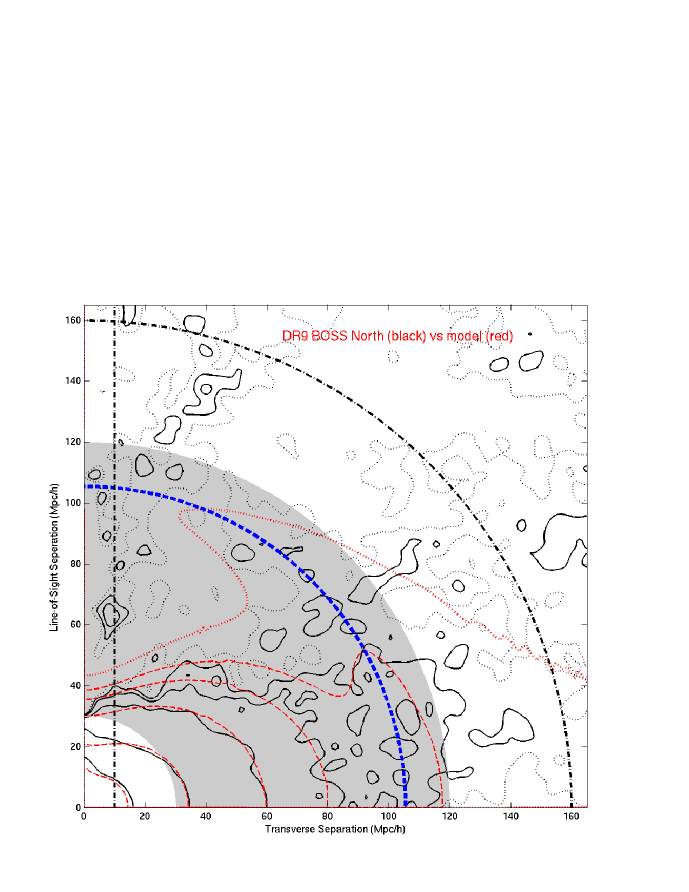
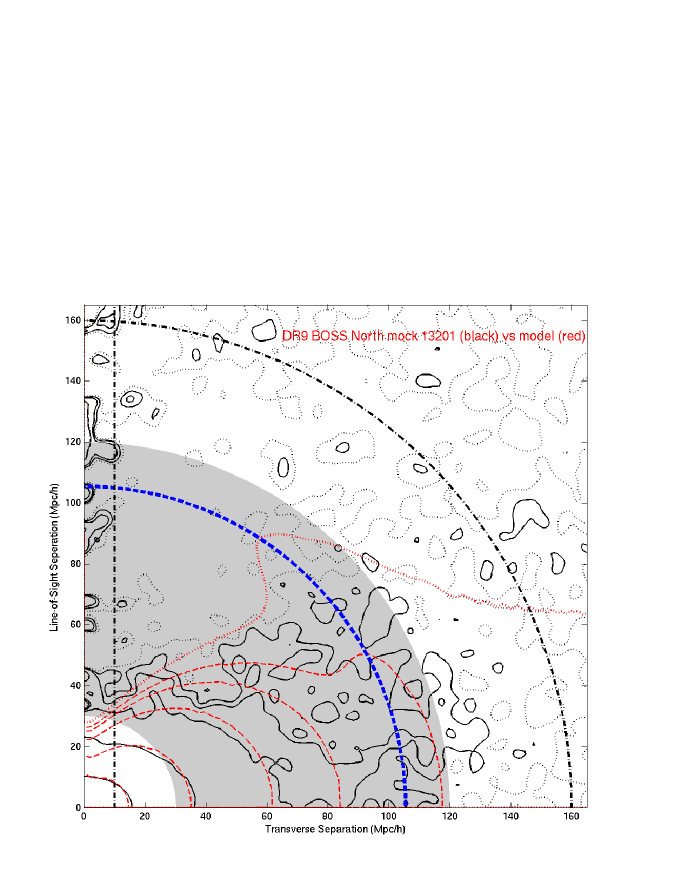
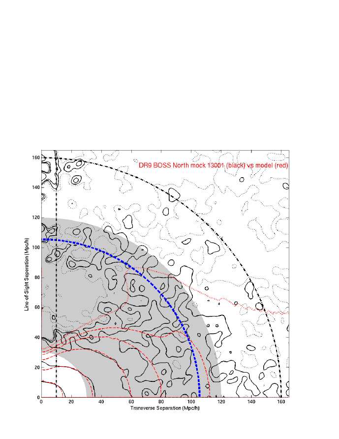
Figure 1: The DR9 BOSS North CMASS sample (upper panel) and two representative mocks (middle and lower panels). The contour levels are $\xi=0.005,0.01,0.025,0.1,0.5$, and the dotted contours denote $\xi\leq 0$. The solid lines are the data (or mock data), and the dashed lines are our model (with parameters chosen from within 68% C.L. marginalized intervals).

Figure 1 shows the DR9 BOSS North CMASS sample (upper panel) and two mocks (middle and lower panels). The contour levels are $\xi=0.005,0.01,0.025,0.1,0.5$, and the dotted contours denote $\xi\leq 0$. The solid lines are the data (or mock data), and the dashed lines are our model (with parameters chosen from within 68% C.L. marginalized intervals). The mock in the middle panel has been chosen because it resembles the data, but it is somewhat noisier than the data on small scales, The mock in the lower panel is the first mock from the suite of mocks; it is noisier than the data on all scales.

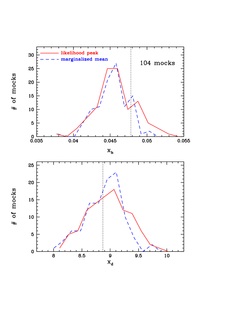
Fig.2 shows the distribution of $x_{h}=H(0.57)\,r_{s}(z_{d})/c$ and $x_{d}=D_{A}(0.57)/r_{s}(z_{d})$ from 104 mocks of the DR9 BOSS North and South CMASS samples. The solid and dashed lines denote the likelihood peaks and marginalized means respectively. The dotted lines indicate the values predicted by the true model of the mocks (the fiducial model assumed for the analysis of actual data). The true values of $x_{h}$ and $x_{d}$ are within the central 68.3% range of the recovered values. This validates out methodology.

Figure 2: The distribution of $x_{h}=H(0.57)\,r_{s}(z_{d})/c$ and $x_{d}=D_{A}(0.57)/r_{s}(z_{d})$ from 104 mocks of the DR9 BOSS North and South CMASS samples. The solid and dashed lines denote the likelihood peaks and marginalized means respectively. The dotted lines indicate the values predicted by the true model of the mocks (the fiducial model assumed for the analysis of actual data).

3.2 Results from BOSS DR9 CMASA Samples

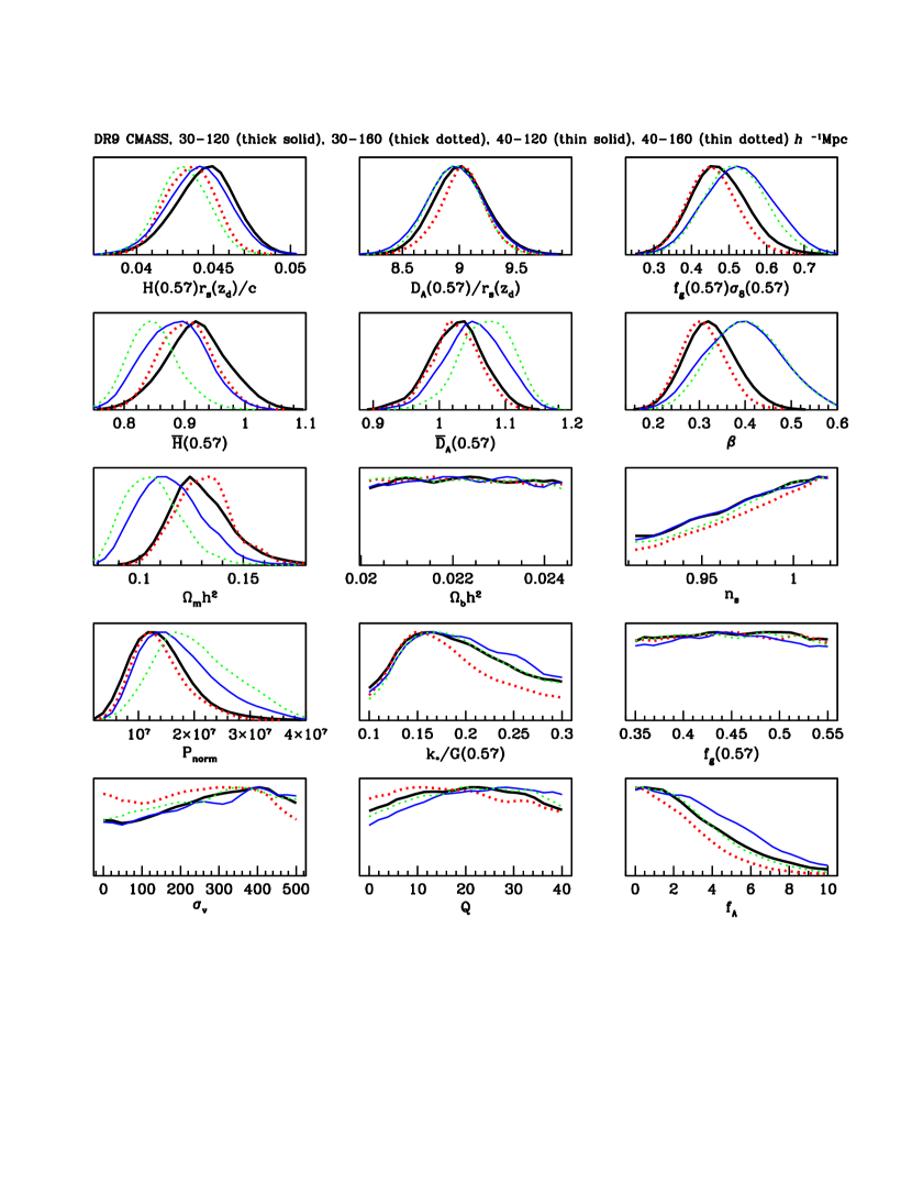
We now present our results from analyzing the real data. Fig.3 shows the 1D marginalized probability distribution of parameters estimated from DR9 BOSS North and South CMASS samples. The different line types denote different scale ranges used in our analysis: 30-120$\,h^{-1}$Mpc (thick solid); 30-160$\,h^{-1}$Mpc (thick dotted); 40-120$\,h^{-1}$Mpc (thin solid); 40-160$\,h^{-1}$Mpc (thin dotted). Fig.4 shows the corresponding 2D joint confidence contours (68% and 95%) of the parameters, with the same line types as in Fig.3. Only the key parameters and parameters with significant correlations are shown in Fig.4.

Figure 3: The 1D marginalized probability distribution of parameters estimated from DR9 BOSS North and South CMASS samples. The different line types denote different scale ranges used in our analysis: 30-120$\,h^{-1}$Mpc (thick solid); 30-160$\,h^{-1}$Mpc (thick dotted); 40-120$\,h^{-1}$Mpc (thin solid); 40-160$\,h^{-1}$Mpc (thin dotted).

Figure 4: The 2D joint confidence contours (68% and 95%) of the parameters estimated from DR9 BOSS North and South CMASS samples, with the same line types as in Fig.3. Only the key parameters and parameters with significant correlations are shown.

Clearly, the data on larger scales, 120-160$\,h^{-1}$Mpc, do not add significant amount of information to the parameter estimation. This is because data on the scale range of 120-160$\,h^{-1}$Mpc is very noisy (see Fig.1). Table 1 lists the $\chi^{2}_{min}$ for the scale ranges that we have considered. Note that the number of fitted parameters is 12. The addition of data on the scale range of 120-160$\,h^{-1}$Mpc significantly increases the $\chi^{2}$ per degree of freedom.

scale range	$N_{data}$	$\chi^{2}_{min}$	$\chi^{2}_{min,pdf}$
30-120$\,h^{-1}$Mpc	208	225.97	1.15
30-160$\,h^{-1}$Mpc	390	529.17	1.40
40-120$\,h^{-1}$Mpc	198	214.29	1.15
40-160$\,h^{-1}$Mpc	380	511.97	1.39

Table 1: The $\chi^{2}_{min}$ for the four different scale ranges of the SDSS DR9 BOSS CMASS samples. Note that the number of fitted parameters is 12.

On the other hand, the inclusion of data on the scale of 30-40$\,h^{-1}$Mpc is critical to placing a tight constraint on $\beta$ (see Fig.3); this is as expected, since more information on RSD comes from smaller scales, where the measured 2DCF is smooth. Tighter constraints on $\beta$ leads to tighter constraints on $H(0.57)$, $D_{A}(z)$, and $f_{g}(0.57)\sigma_{8}(0.57)$ due to parameter correlations (see Fig.3). We do not use the scale range below 30$\,h^{-1}$Mpc, where our current model is not expected to fit well as we have not included modeling for the mixing of nonlinearity and RSD on the smallest scales.

We choose the results from scale range of $30-120\,h^{-1}$Mpc as our fiducial results, as they are less affected by noisy data, and retain the information on RSD. Tables 2 and 3 give the marginalized means and the normalized covariance matrix for the key parameters that we have measured or derived from measurements. Table 2 also includes results from using the scale range of $30-160\,h^{-1}$Mpc for comparison.

	$30<s<120$	$30<s<160$
$H(0.57)$	86.14 $\pm$ 4.77	84.52$\pm$4.04
$D_{A}(0.57)$	1396.11 $\pm$ 53.17	1394.04$\pm$47.64
$\Omega_{m}h^{2}$	0.130 $\pm$ 0.015	0.131$\pm$ 0.014
$\beta$	0.326 $\pm$ 0.055	0.309$\pm$ 0.048
$H(0.57)\,r_{s}(z_{d})/c$	0.0444$\pm$0.0019	0.0435 $\pm$ 0.015
$D_{A}(0.57)/r_{s}(z_{d})$	9.01 $\pm$ 0.23	9.02$\pm$ 0.20
$f(0.57)\,\sigma_{8}(0.57)$	0.474 $\pm$ 0.075	0.457$\pm$ 0.065

Table 2: The mean and standard deviation of $\{H(0.57)$, $D_{A}(0.57)$, $\Omega_{m}h^{2}$, $\beta$, $H(0.57)\,r_{s}(z_{d})/c$, $D_{A}(0.57)/r_{s}(z_{d})$, $f(0.57)\,\sigma_{8}(0.57)\}$ from SDSS DR9 CMASS samples, for the scale ranges $30<s<120h^{-1}$Mpc and $30<s<160h^{-1}$Mpc. The unit of $H$ is $\,{\rm km}\,{\rm s}^{-1}\,{\rm Mpc}^{-1}$. The unit of $D_{A}$ is $\rm Mpc$.

	$H(0.57)$	$D_{A}(0.57)$	$\Omega_{m}h^{2}$	$\beta$	$H(0.57)\,r_{s}(z_{d})/c$	$D_{A}(0.57)/r_{s}(z_{d})$	$f(0.57)\sigma_{8}(0.57)$
$H(0.57)$	1.0000	-0.4659	0.6794	0.1742	0.8535	0.0432	0.0102
$D_{A}(0.57)$	-0.4659	1.0000	-0.7592	0.4076	-0.0980	0.6535	0.5375
$\Omega_{m}h^{2}$	0.6794	-0.7592	1.0000	-0.2659	0.2189	-0.0419	-0.2451
$\beta$	0.1742	0.4076	-0.2659	1.0000	0.4056	0.3158	0.9008
$H(0.57)\,r_{s}(z_{d})/c$	0.8535	-0.0980	0.2189	0.4056	1.0000	0.0403	0.1771
$D_{A}(0.57)/r_{s}(z_{d})$	0.0432	0.6535	-0.0419	0.3158	0.0403	1.0000	0.5333
$f(0.57)\sigma_{8}(0.57)$	0.0102	0.5375	-0.2451	0.9008	0.1771	0.5333	1.0000

Table 3: Normalized covariance matrix of the measured and derived parameters, $\{H(0.57)$, $D_{A}(0.57)$, $\Omega_{m}h^{2}$, $\beta,$, $H(0.57)\,r_{s}(z_{d})/c$, $D_{A}(0.57)/r_{s}(z_{d})$, $f(0.57)\sigma_{8}(0.57)\}$ from SDSS DR9 CMASS samples for the scale ranges $30<s<120h^{-1}$Mpc.

4 Summary and Discussion

We have analyzed the anisotropic two dimensional galaxy correlation function (2DCF) of the CMASS galaxy samples from the Sloan Digital Sky Survey Data Release 9 (DR9) of the Baryon Oscillation Spectroscopic Survey (BOSS) data, and derived robust constraints on $H(0.57)r_{s}(z_{d})/c$, $D_{A}(0.57)/r_{s}(z_{d})$, and $f_{g}(0.57)\sigma_{8}(0.57)$ (see Table 2 and Table 3). While consistent with previous results using the same data, our results have significantly better precision since we are using all the information from the 2DCF in the scale range of interest. Since our measurements have been marginalized over sufficiently wide priors for the relevant parameters; they can be combined with other data to probe dark energy and gravity.

We found that the data beyond the scale of 120 $h^{-1}$Mpc are dominated by noise (see Table 1). On the other hand, the inclusion of data below the scale of 40 $h^{-1}$Mpc is important for constraining the redshift-space distortion parameter, and hence of the growth rate (see Fig.3). We have chosen the scale range of 30 to 120 $h^{-1}$Mpc (the quasilinear and linear scales at $z=0.57$) in obtaining our fiducial results.

We do not use the scale range below 30$\,h^{-1}$Mpc, where our current model is not expected to fit well as we have not included modeling for the mixing of nonlinearity and RSD on the smallest scales. The more advanced modeling that would apply to clustering on smaller scales cannot be validated using the BOSS DR9 mocks, as these were produced using a second-order Lagrangian perturbation theory (2LPT) method, and were calibrated to reproduce the clustering measurements between 30 and 80$\,h^{-1}$Mpc (Manera et al., 2013). Fig.1 shows that our model fits the data and the mocks well in the scale range used (indicated by the gray band), and for transverse separations greater than 10 $\,h^{-1}$Mpc for the mocks. We carried out MCMC runs with and without making the transverse cut at $\sigma\geq 10\,h^{-1}$Mpc, and found that they give very similar results. This may be due to the fact that the cut would only remove a relatively small number of data points (our bin size is 10$\,h^{-1}$Mpc x 10$\,h^{-1}$Mpc).

Note that the results from the BOSS DR9 CMASS north and south samples have significantly smaller measurement uncertainties compared to the expectation based on the distribution of the results from the mocks (compare Fig.3 and Fig.2). This may be due to the fact that the measured 2DCF appears less noisy that those measured from the mocks (see Fig.1), which reflects a statistical property of the data.

Linder et al. (2014) presented another independent analysis of DR9 BOSS data, using the method from Song, Okumura, Taruya (2014), which is a similar approach with a different theoretical model. The main difference in methodology is that Linder et al. (2014) effectively fixed the shape of $P(k)$, while we marginalize over the shape of $P(k)$ by marginalizing over $\Omega_{m}h^{2}$, $\Omega_{b}h^{2}$, and $n_{s}$. Our results are broadly similar to that of Linder et al. (2014), with the main difference being that Linder et al. (2014) measured $H(0.57)$, $D_{A}(0.57)$, and $G_{\Theta}$ with either WMAP9 or Planck priors, while our measurements are independent of the CMB priors.

Our measurements of $H(0.57)$ and $D_{A}(0.57)$ are consistent with the expected values from WMAP9 (Bennett et al., 2013) at 68% confidence level. Spergel, Flauger, & Hlozek (2013) showed that Planck results (Ade et al., 2013) may be sensitive to systematic effects; they found that the difference between Planck and WMAP 9 results are significantly reduced once the Planck data are cleaned in a consistent and systematic manner.

The latest BOSS data (DR11) seem to give much more stringent results than DR9 (see Anderson et al. (2013); Chuang et al. (2013); Samushia et al. (2013); Sanchez et al. (2013)). It will be interesting to apply our method to BOSS DR11 data, once they are publicly available. As sufficiently large mock catalogues become available, we will be able to further validate our methodology for application to the Euclid GC data.

References

• (1)
• Ade et al. (2013) Ade, P.A.R., et al. 2013, arXiv:1303.5076
• Anderson et al. (2012) Anderson, L., et al. 2012, MNRAS, 427, 3435
• Anderson et al. (2013) Anderson, L., et al. 2013, arXiv:1312.4877
• Bennett et al. (2013) Bennett, Cl., et al. 2013, ApJS, 208, 20
• Blake & Glazebrook (2003) Blake C., Glazebrook G. 2003, ApJ 594, 665
• Caldwell & Kamionkowski (2009) Caldwell, R. R., & Kamionkowski, M., 2009, Ann.Rev.Nucl.Part.Sci., 59, 397
• Chuang & Wang (2012) Chuang C.-H., Wang Y. 2012, MNRAS 426, 226
• Chuang & Wang (2013) Chuang C.-H., Wang Y. 2013, MNRAS, 435, 255
• Chuang, Wang, & Hemantha (2012) Chuang, C.-H., Wang Y., Hemantha M. 2012, MNRAS 423, 1474
• Chuang et al. (2013) Chuang, C.-H., et al. 2013, arXiv:1312.4889
• Cole et al. (2005) Cole, S., et al., 2005, MNRAS, 362, 505
• Eisenstein & Hu (1998) Eisenstein, D.Β J.; and Hu, W., ApJ, 496, 605 (1998)
• Eisenstein, Seo, & White (2007) Eisenstein, D. J.; Seo, H.-J.; White, M. 2007, ApJ, 664, 660
• Fixsen (2009) Fixsen, D.J. 2009, ApJ, 707, 916
• Frieman, Turner, & Huterer (2008) Frieman, J., Turner, M., Huterer, D., ARAA, 46, 385 (2008)
• Guzzo et al. (2008) Guzzo L. et al. 2008, Nature 451, 541
• Hamilton (1992) Hamilton, A.Β J.Β S., 1992, APJL, 385, L5
• Hemantha, Wang, & Chuang (2013) Hemantha, M. D. P.; Wang, Y.; Chuang, C.-H., arXiv:1310.6468
• Kaiser (1987) Kaiser N., 1987, MNRAS 227, 1
• Landy (2002) Landy, S.Β D., ApJ, 567, L1
• Landy & Szalay (1993) Landy, S.Β D. and Szalay, A.Β S. 1993, ApJ, 412, 64
• Laureijs et al. (2011) Laureijs R. et al. 2011, β€œEuclid Definition Study Report”, arXiv:1110.3193
• Lewis & Bridle (2002) Lewis, A. and Bridle, S., Phys.Β Rev.Β  D 66, 103511 (2002)
• Li et al. (2011) Li, M.; Li, X.-D.; Wang, S.; Wang, Y., 2011, Commun.Theor.Phys., 56, 525
• Linder et al. (2014) Linder, E.V.; Oh, M.; Okumura, T.; Sabiu, C. G.; Song, Y.-S. 2014, Phys. Rev. D 89, 063525
• Manera et al. (2013) Manera, M., et al. 2013, MNRAS, 428, 1036
• Mehta et al. (2012) Mehta, K., et al., 2012, MNRAS, 427, 2168
• Perlmutter et al. (1999) Perlmutter S. et al. 1999, ApJ 517, 565
• Press et al. (1992) Press W.H., Teukolsky S,A., Vetterling W.T., Flannery B.P., 1992, Numerical recipes in C. The art of scientific computing, Second edition, Cambridge University Press.
• Ratcliffe et al. (1998) Ratcliffe, A., etΒ al., 1998, VizieR Online Data Catalog, 730, 417
• Ratra & Vogeley (2008) Ratra, B., Vogeley, M.Β S., 2008, Publ.Astron.Soc.Pac., 120, 235
• Riess et al. (1998) Riess A. et al. 1998, AJ 116, 1009
• Samushia et al. (2013) Samushia, L., et al., 2013, arXiv:1312.4899
• Sanchez, Baugh, & Angulo (2008) Sanchez, Ariel G.; Baugh, C. M.; Angulo, R. 2008, MNRAS, 390, 1470
• Sanchez et al. (2013) Sanchez, A.G., 2013, arXiv:1312.4854
• Seo & Eisenstein (2003) Seo H., Eisenstein D. 2003, ApJ 598, 720
• Song & Percival (2009) Song, Y.-S.; & Percival, W.J. 2009, JCAP, 0910, 004
• Song, Okumura, Taruya (2014) Song, Y.S.; Okumura, T.; & Taruya, A., Phys. Rev. D 89, 103541 (2014)
• Spergel, Flauger, & Hlozek (2013) Spergel, D.; Flauger, R.; Hlozek, R., arXiv:1312.3313
• Uzan (2010) Uzan, J.-P. 2010, General Relativity and Gravitation, 42, 2219
• Wang (2008) Wang Y. 2008, JCAP 0805, 021
• Wang (2010) Wang, Y., Dark Energy, Wiley-VCH (2010)
• Wang & Wang (2013) Wang, Y.; Wang, S. 2013, Phys. Rev. D 88, 043522
• Wang, Chuang, & Hirata (2013) Wang, Y.; Chuang, C.-H.; Hirata, C.M., 2013, MNRAS, 430, 2446
• Weinberg et al. (2013) Weinberg, D. H.; Mortonson, M. J.; Eisenstein, D.J.; Hirata, C.; Riess, A. G.; Rozo, E 2013, Physics Reports, 530, 87