Online Bin Stretching with Three Bins

Abstract

Online Bin Stretching is a semi-online variant of bin packing in which the algorithm has to use the same number of bins as an optimal packing, but is allowed to slightly overpack the bins. The goal is to minimize the amount of overpacking, i.e., the maximum size packed into any bin.

We give an algorithm for Online Bin Stretching with a stretching factor of $11/8=1.375$ for three bins. Additionally, we present a lower bound of $45/33=1.\overline{36}$ for Online Bin Stretching on three bins and a lower bound of $19/14$ for four and five bins that were discovered using a computer search.

1 Introduction

The most famous algorithmic problem dealing with online assignment is arguably Online Bin Packing. In this problem, known since the 1970s, items of size between $0$ and $1$ arrive in a sequence and the goal is to pack these items into the least number of unit-sized bins, packing each item as soon as it arrives.

Online Bin Stretching, which was introduced by Azar and Regev in 1998 [3, 4], deals with a similar online scenario. Again, items of size between $0$ and $1$ arrive in a sequence, and the algorithm needs to pack them as soon as each item arrives, but it has two advantages: (i) The packing algorithm knows $m$, the number of bins that an optimal offline algorithm would use, and must also use only at most $m$ bins, and (ii) the packing algorithm can use bins of capacity $R$ for some $R\geq 1$. The goal is to minimize the stretching factor $R$.

While formulated as a bin packing variant, Online Bin Stretching can also be thought of as a semi-online scheduling problem, in which we schedule jobs in an online manner on exactly $m$ machines, before any execution starts. We have a guarantee that the optimum offline algorithm could schedule all jobs with makespan $1$. Our task is to present an online algorithm with makespan of the schedule being at most $R$.

Motivation. We give two of applications of Online Bin Stretching.

Server upgrade. This application has first appeared in [3]. In this setting, an older server (or a server cluster) is streaming a large number of files to the newer server without any guarantee on file order. The files cannot be split between drives. Both servers have $m$ disk drives, but the newer server has a larger capacity of each drive. The goal is to present an algorithm that stores all incoming files from the old server as they arrive.

Shipment checking. A number $m$ of containers arrive at a shipping center. It is noted that all containers are at most $p\leq 100$ percent full. The items in the containers are too numerous to be individually labeled, yet all items must be unpacked and scanned for illicit and dangerous material. After the scanning, the items must be speedily repackaged into the containers for further shipping. In this scenario, an algorithm with stretching factor $100/p$ can be used to repack the objects into containers in an online manner.

History. Online Bin Stretching was proposed by Azar and Regev [3, 4]. Already before this, a matching upper and lower bound of $4/3$ for two bins had appeared [17]. Azar and Regev extended this lower bound to any number of bins and gave an online algorithm with a stretching factor $1.625$.

The problem has been revisited recently, with both lower bound improvements and new efficient algorithms. On the algorithmic side, Kellerer and Kotov [16] have achieved a stretching factor $11/7\approx 1.57$ and Gabay et al. [13] have achieved $26/17\approx 1.53$. The best known general algorithm with stretching factor $1.5$ was presented by the authors of this paper in [8].

In the case with only three bins, the previously best algorithm was due to Azar and Regev [3], with a stretching factor of $1.4$.

On the lower bound side, the lower bound $4/3$ of [3] was surpassed only for the case of three bins by Gabay et al. [11], who show a lower bound of $19/14\approx 1.357$, using an extensive computer search. The preprint [11] was updated in 2015 [12] to include a lower bound of $19/14$ for four bins.

Our contributions. In Section 2 we present an algorithm for three bins of capacity $11/8=1.375$. This is the first improvement of the stretching factor $1.4$ of Azar and Regev [3]. In Section 3, we present a new lower bound of $45/33=1.\overline{36}$ for Online Bin Stretching on three bins, along with a lower bound of $19/14$ on four and five bins which is the first non-trivial lower bound for four and five bins. We build on the paper of Gabay et al. [11] but significantly change the implementation, both technically and conceptually. The lower bound of $19/14$ for four bins is independently shown in [12].

A preliminary version of this work appeared in WAOA 2014 [7] and SOFSEM 2016 [6].

Related work. The NP-hard problem Bin Packing was originally proposed by Ullman [18] and Johnson [15] in the 1970s. Since then it has seen major interest and progress, see the survey of Coffman et al. [9] for many results on classical Bin Packing and its variants. While our problem can be seen as a variant of Bin Packing, note that the algorithms cannot open more bins than the optimum and thus general results for Bin Packing do not translate to our setting.

As noted, Online Bin Stretching can be formulated as the online scheduling on $m$ identical machines with known optimal makespan. Such algorithms were studied and are important in designing constant-competitive algorithms without the additional knowledge, e.g., for scheduling in the more general model of uniformly related machines [2, 5, 10].

For scheduling, also other types of semi-online algorithms are studied. Historically first is the study of ordered sequences with non-decreasing processing times [14]. Most closely related is the variant with known sum of all processing times studied in [17] and the currently best results are a lower bound of $1.585$ and an algorithm with ratio $1.6$, both from [1]. Note that this shows, somewhat surprisingly, that knowing the actual optimum gives a significantly bigger advantage to the online algorithm over knowing just the sum of the processing times (which, divided by $m$, is a lower bound on the optimum).

Definitions and notation. Our main problem, Online Bin Stretching, can be described as follows:

Input: an integer $m$ and a sequence of items $I=i_{1},i_{2},\ldots$ given online one by one. Each item has a size $s(i)\in[0,1]$ and must be packed immediately and irrevocably. It is guaranteed that there exists a packing of all items in $I$ into $m$ bins of capacity $1$.

Parameter: The stretching factor $R\geq 1$.

Output: Partitioning (packing) of $I$ into bins $B_{1},\ldots,B_{m}$ so that $\sum_{i\in B_{j}}s(i)\leq R$ for all $j=1,\ldots,m$.

Goal: Design an online algorithm with the stretching factor $R$ as small as possible which packs all input sequences satisfying the guarantee.

For a bin $B$, we define the size of the bin $s(B)=\sum_{i\in B}s(i)$. Unlike $s(i)$, $s(B)$ can change during the course of the algorithm, as we pack more and more items into the bin. To easily differentiate between items, bins and lists of bins, we use lowercase letters for items ($i$, $b$, $x$), uppercase letters for bins and other sets of items ($A$, $B$, $X$), and calligraphic letters for lists of bins (${\mathcal{A}}$, ${\mathcal{C}}$, ${\mathcal{L}}$).

We rescale the item sizes and bin capacities for simplicity. Therefore, in our setting, each item has an associated size $s(i)\in[0,k]$, where $k\in\mathbb{N}$ is also the capacity of the bins which the optimal offline algorithm uses. The online algorithm for Online Bin Stretching uses bins of capacity $t\in\mathbb{N}$, $t\geq k$. The resulting stretching factor is thus $t/k$.

2 Algorithm

We scale the input sizes by $16$. The stretched bins in our setting therefore have capacity $22$ and the optimal offline algorithm can pack all items into three bins of capacity $16$ each. We prove the following theorem.

Theorem 2.1

There exists an algorithm that solves Online Bin Stretching for three bins with stretching factor $1+3/8=1.375$.

The three bins of our setting are named $A$, $B$, and $C$. We exchange the names of bins sometimes during the course of the algorithm.

A natural idea is to try to pack first all items in a single bin, as long as possible. In general, this is the strategy that we follow. However, somewhat surprisingly, it turns out that from the very beginning we need to put items in two bins even if the items as well as their total size are relatively small.

It is clear that we have to be very cautious about exceeding a load of 6. For instance, if we put 7 items of size 1 in bin $A$, and 7 such items in $B$, then if two items of size 16 arrive, the algorithm will have a load of at least 23 in some bin. Similarly, we cannot assign too much to a single bin: putting 20 items of size 0.5 all in bin $A$ gives a load of 22.5 somewhere if three items of size 12.5 arrive next. (Starting with items of size 0.5 guarantees that there is a solution with bins of size 16 at the end.)

On the other hand, it is useful to keep one bin empty for some time; many problematic instances end with three large items such that one of them has to be placed in a bin that already has high load. Keeping one bin free ensures that such items must have size more than 11 (on average), which limits the adversary’s options, since all items must still fit into bins of size 16.

Deciding when exactly to start using the third bin and when to cross the threshold of 6 for the first time was the biggest challenge in designing this algorithm: both of these events should preferably be postponed as long as possible, but obviously they come into conflict at some point.

2.1 Good situations

Before stating the algorithm itself, we list a number of good situations (GS). These are configurations of the three bins which allow us to complete the packing regardless of the following input.

It is clear that the identities of the bins are not important here; for instance, in the first good situation, all that we need is that any two bins together have items of size at least 26. We have used names only for clarity of presentation and of the proofs.

Definition 1

A partial packing of an input sequence $S$ is a function $p:S_{1}\to\{A,B,C\}$ that assigns a bin to each item from a prefix $S_{1}$ of the input sequence $S$.

Good Situation 1

Given a partial packing such that $s(A)+s(B)\geq 26$ and $s(C)$ is arbitrary, there exists an online algorithm that packs all remaining items into three bins of capacity $22$.

Proof

Since the optimum can pack into three bins of size $16$, the total size of items in the instance is at most $3\cdot 16=48$. If two bins have size $s(A)+s(B)\geq 26$, all the remaining items (including the ones already placed on $C$) have size at most $22$. Thus we can pack them all into bin $C$. ∎

Good Situation 2

Given a partial packing such that $s(A)\in[4,6]$ and $s(B)$ and $s(C)$ are arbitrary, there exists an online algorithm that packs all remaining items into three bins of capacity $22$.

Proof

Let $A$ be the bin with size between $4$ and $6$ and $B$ be one of the other bins (choose arbitrarily). Put all the items greedily into $B$. When an item does not fit, put it into $A$, where it fits, as originally $s(A)$ is at most $6$. Now the size of all items in $B$ plus the last item is at least $22$. In addition, $A$ has items of size at least $4$ before the last item by the assumption. Together we have $s(A)+s(B)\geq 26$, allowing us to apply GS1. ∎

From now on, we assume that each bin $X\in\{A,B,C\}$ satisfies $s(X)\not\in[4,6]$, otherwise we reach GS2.

Good Situation 3

Given a partial packing such that $s(A)\geq 15$ and either (i) $s(B)+s(C)\geq 22$ or (ii) $s(C)<4$ and $s(B)$ is arbitrary, there exists an online algorithm that packs all remaining items into three bins of capacity $22$.

Proof

(i) We have $\max(s(B),s(C))\geq 11$, so we are in GS1 on bins $A$ and $B$ or on bins $A$ and $C$.

(ii) We pack arriving items into $B$. If $s(B)\geq 11$ at any time, we apply GS1 on bins $A$ and $B$. Thus we can assume $s(B)<11$ and we cannot continue packing into $B$ any further. This implies that an item $i$ arrives such that $s(i)>11$. As $s(C)<4$, we pack $i$ into it and apply GS1 on bins $A$ and $C$.∎

Good Situation 4

Given a partial packing such that $s(A)+s(B)\geq 15+\frac{1}{2}s(C)$, $s(B)<4$, and $s(C)<4$, there exists an online algorithm that packs all remaining items into three bins of capacity $22$.

Proof

Let $c$ be the value of $s(C)$ when the conditions of this good situation hold for the first time. We run the following algorithm until we reach GS1 or GS3:

(1) If the incoming item $i$ has $s(i)\geq 11-\frac{1}{2}c$, pack $i$ into $B$. (2) Else, if $i$ fits on $A$, pack it there. (3) Otherwise pack $i$ into $C$.

If at any time an item $i$ is packed into $B$ (where it always fits), then $s(A)+s(B)\geq 26$ and we reach GS1. In the event that no item $i$ is packed into $B$, we reach GS3 (with $B$ in the role of $C$) whenever the algorithm brings the size of $A$ to or above 15.

The only remaining case is when $s(A)<15$ throughout the algorithm and several items with size in the interval $I\mathrel{\hbox to0.0pt{\raisebox{1.29167pt}{$\cdot$}\hss}\raisebox{-1.29167pt}{$\cdot$}}=(22-s(A),11-\frac{1}{2}c)$ arrive. These items are packed into $C$. Note that $I\subseteq(7,11)$ and that the lower bound of $I$ may decrease during the course of the algorithm.

The first two items with size in $I$ will fit together, since $2(11-\frac{1}{2}c)+c=22$. With two such items packed into $C$, we know that the load $s(A)+s(C)$ is at least $s(A)+2(22-s(A))=44-s(A)>29$ and we have reached GS1, finishing the analysis. ∎

Good Situation 5

Given a partial packing such that an item $a$ with $s(a)>6$ is packed into bin $A$, $s(B)\in[3,4)$, and $C$ is empty, there exists an algorithm that packs all remaining items into three bins of capacity $22$.

Proof

Pack all incoming items into $A$ as long as it possible. If $s(A)\geq 12$, we have GS4, and so we assume the contrary. Therefore, $s(A)<12$ and an item $i$ arrives which cannot be packed into $A$.

Place $i$ into $B$. If $s(i)\geq 12$, we apply GS3. We thus have $s(i)\in(10,12)$ and $s(A)\geq 22-s(i)>10$. Continue with First Fit on bins $B$, $A$, and $C$ in this order.

We claim that GS1 is reached at the latest after First Fit has packed two items, $x$ and $y$, on bins other than $B$. If one of them (say $x$) is packed into bin $A$, this holds because $s(x)+s(B)>22$ and $s(A)>10$ already before this assignment – enough for GS1. If both items do not fit in $A$, they are both larger than 10, since $s(A)<12$. We will show by contradiction that this cannot happen.

As $s(A)<12$ from our previous analysis, we note that $s(x),s(y)>10$. We therefore have three items $i,x,y$ with $s(i),s(x),s(y)>10$ and an item $s(a)>6$ from our initial conditions. These four items cannot be packed together by any offline algorithm into three bins of capacity 16, and so we have a contradiction with $s(x),s(y)>10$. ∎

Good Situation 6

If $s(C)<4$, $s(B)>6$ and $s(A)\geq s(B)+4-s(C)$, there exists an algorithm that packs all remaining items into three bins of capacity $22$.

Proof

Pack all items into $A$, until an item $x$ does not fit. At this point $s(A)+x>22$. If $x$ fits on $B$, we put it there and reach GS1 because $s(B)>6$. Otherwise, $x$ definitely fits on $C$ because $s(C)<4$. By the condition on $s(A)$, we have $x+s(A)+s(C)\geq x+s(B)+4>26$, and we are in GS1 again. ∎

Good Situation 7

Suppose $s(A)<4$, $s(C)<4$. If $s(B)\leq 9+\frac{1}{2}(s(A)+s(C))$ and for a new item $x$ we have $s(B)+s(x)>22$, then there exists an online algorithm that packs all remaining items into three bins of capacity $22$.

Proof

We have $s(B)>22-s(x)>6$ and $s(x)>22-s(B)\geq 13-\frac{1}{2}(s(A)+s(C))\geq s(B)+4-s(A)-s(C)$. Placing $x$ on $A$ we increase the size of $A$ to at least $s(B)+4-s(C)$ and we reach GS6. ∎

2.2 Good Situation First Fit

Throughout our algorithm, we often use a special variant of First Fit which tries to reach good situations as early as possible. This variant can be described as follows:

Definition 2

Let ${\mathcal{L}}=(X|_{k},Y|_{l},\ldots)$ be a list of bins $X,Y,\ldots$ where each bin $X$ has an associated capacity $k$ satisfying $s(X)\leq k$. GSFF(${\mathcal{L}}$) (Good Situation First Fit) is an online algorithm for bin stretching that works as follows:

Subroutine GSFF(${\mathcal{L}}$): For each item $i$: If it is possible to pack $i$ into any bin (including bins not in ${\mathcal{L}}$, and using capacities of 22 for all bins) such that a good situation is reached, do so and continue with the algorithm of the relevant good situation. Otherwise, traverse the list ${\mathcal{L}}$ in order and pack $i$ into the first bin $X$ such that $X|_{k}\in{\mathcal{L}}$ and $s(X)+s(i)\leq k$. If there is no such bin, stop.

For example, GSFF($A|_{4},B|_{22}$) checks whether either $(A\cup\{j\},B,C)$, $(A,B\cup\{j\},C)$ or $(A,B,C\cup\{j\})$ is a partial packing of any good situation. If this is not the case, the algorithm packs $j$ into bin $A$ provided that $s(A)+s(j)\leq 4$. If $s(A)+s(j)>4$, the algorithm packs $j$ into bin $B$ with capacity $22$. If $j$ cannot be placed into $B$, GSFF($A|_{4},B|_{22}$) halts and another online algorithm must be applied to pack $j$ and subsequent items.

2.3 The algorithm

In a way, any algorithm for online bin stretching for three bins must be designed so as to avoid several bad situations: the two most prominent ones being either two items of size $R/2$ or three items of size $R/3$, where $R$ is the volume of the remaining items.

Our algorithm – especially Steps (4) and (10) – are designed to primarily evade such bad situations, while making sure that no good situation is missed. This evasive nature gives it its name.

Algorithm Evasive: (1) Run GSFF($A|_{4},B|_{4}$). (2) Rename the bins so that $s(A)\geq s(B)$. (3) If the next item $j$ satisfies $s(j)>6$: (4) Set $p\mathrel{\hbox to0.0pt{\raisebox{1.29167pt}{$\cdot$}\hss}\raisebox{-1.29167pt}{$\cdot$}}=6+s(j)$; apply GSFF($A|_{p},B|_{4}$). (5) If the next item $w$ fits into $A|_{22}$: (6) GSFF($A|_{22},B|_{22},C|_{22}$). (7) Else: (8) GSFF($A|_{p},B|_{22},C|_{22}$). (9) Else ($j$ satisfies $s(j)<4$): (10) GSFF($A|_{4},B|_{q},C|_{4}$) where $q\mathrel{\hbox to0.0pt{\raisebox{1.29167pt}{$\cdot$}\hss}\raisebox{-1.29167pt}{$\cdot$}}=9+\frac{1}{2}(s(A)+s(C))$. Update $q$ whenever $s(A)$ or $s(C)$ changes. (11) GSFF($A|_{4},B|_{22},C|_{22}$). (12) GSFF($A|_{22},B|_{22},C|_{22}$).

2.4 Analysis

Let us start the analysis of the algorithm Evasive in Step (3), where the algorithm branches on the size of the item $j$.

Throughout the proof, we will need to argue about loads of the bins $A$, $B$, $C$ before various items arrived. The following notation will help us in this endeavour:

Notation. Suppose that $A$ is a bin and $x$ is an item that gets packed at some point of the algorithm (not necessarily into $A$). Then $A_{\leftarrow x}$ will indicate the set of items that are packed into $A$ just before $x$ arrived.

We first observe that our algorithm can be in two very different states, based on whether $s(j)>6$ or $s(j)<4$. Note that the case $s(j)\in[4,6]$ is immediately settled using GS2.

Observation 2.2

Assume that $s(j)<4$. We have $s(A_{\leftarrow j})\in(3,4)$ and $s(B_{\leftarrow j})+s(j)\in(6,8)$ where $A$ and $B$ are bins after renaming in Step (2). Thus both $A$ and $B$ received some items during Step (1). Moreover, there is at most one item either in $A_{\leftarrow j}$, or in $B_{\leftarrow j}$.

Proof

Since $s(j)<4$ and $s(B_{\leftarrow j})<4$, the item $j$ is assigned to $B$ in Step (10), which by Step (2) is the least loaded bin among $A$ and $B$ after Step (1). For this bin, we have $s(B_{\leftarrow j})>2$, else we reach GS2. This implies that both $A$ and $B$ received items in Step (1), so $s(A_{\leftarrow j})+s(B_{\leftarrow j})>6$, else a good situation would have been reached before $j$ arrived. It follows that $s(A_{\leftarrow j})\in(3,4)$ and $s(B_{\leftarrow j})+s(j)\in(6,8)$.

Since any item that is put into $B$ during Step (1) must have size of more than two (otherwise it fits into $A|_{6}$), only one such item can be packed into $B$ which proves the last statement.∎

Contrast the previous observation with the next one, which considers $s(j)>6$:

Observation 2.3

Assume that $s(j)>6$. Then, $s(A_{\leftarrow j})<3$, $s(B_{\leftarrow j})=0$.

Proof

If $s(A_{\leftarrow j})\geq 3$ we reach GS5 by packing $j$ into $B$. However, if $s(A_{\leftarrow j})<3$ then $s(A_{\leftarrow j})+s(B_{\leftarrow j})<6$ which can be true (without reaching a good situation) only if $s(B_{\leftarrow j})=0$. ∎

Both the analysis and the algorithm differ quite a lot based on the size of $j$. If it holds that $s(j)>6$, we enter the large case of the analysis, while $s(j)<4$ will be analyzed as the standard case. Intuitively, if $s(j)>6$, the offline optimum is now constrained as well; for instance, no three items of size $10$ can arrive in the future. This makes the analysis of the large case comparatively simpler.

2.5 The large case

We now assume that $s(j)>6$. Our goal in both the large case and the standard case will be to show that in the near future either a good situation is reached or several large items arrive, but Evasive is able to pack them nonetheless.

Let us start by recalling the relevant steps of the algorithm:

(4) Set $p\mathrel{\hbox to0.0pt{\raisebox{1.29167pt}{$\cdot$}\hss}\raisebox{-1.29167pt}{$\cdot$}}=6+s(j)$; apply GSFF($A|_{p},B|_{4}$). (5) If the next item $w$ fits into $A|_{22}$: (6)      GSFF($A|_{22},B|_{22},C|_{22}$). (7) Else: (8)      GSFF($A|_{p},B|_{22},C|_{22}$)

By choosing the limit $p$ to be $s(j)+6$ in Step (4), we make enough room for $j$ to be packed into $A$. We also ensure that any item $i$ larger than $6$ that cannot be placed into $A$ with capacity 22 must satisfy $s(i)+s(j)>16$ and so $i$ cannot be with $j$ in the same bin in the offline optimum packing.

Let us define $A_{S}$ as the set of items on $A$ of size less than $6$ (packed before or after $j$). We note the following:

Observation 2.4

1. During Step (4), if $B$ contains any item, it is true that $s(A_{S})+s(B)>6$.

2. If no good situation is reached, the item $w$ ending Step (4) satisfies $s(w)>6$.

Proof

The first point follows immediately from our choice of $p$ and GSFF($A|_{p},B|_{4}$).

For the second part of the observation, consider the item $w$ that ends Step (4) and assume $s(w)\leq 6$. The possibility that $s(w)\in[4,6]$ is excluded due to GS2. The case $s(B_{\leftarrow w})\geq 3$ is also excluded, as this would imply GS5 with $j$ in $A$.

Since $s(B_{\leftarrow w})+s(w)>6$, the only remaining possibility is $s(B_{\leftarrow w})\in[2,3),s(w)\in(3,4)$. Even though $w$ does not fit into $A|_{p}$, if we were to pack $w$ into $A|_{22}$, we can use the first point of this observation and get $s(A)+s(B)\geq s(j)+\big{(}s(A_{S})+s(B_{\leftarrow w})\big{)}+s(w)>6+6+3=18$, enough for GS4. The algorithm GSFF($A|_{p},B|_{4}$) in Step (4) will notice this possibility and will pack $w$ into $A$, where it will always fit, as $s(A_{\leftarrow w})<15$ by GS4. ∎

We now split the analysis based on which branch is entered in Step (5):

Case 1: Item $w$ fits into bin $A$; we enter Step (6).

We first note that $s(A)+s(B)<15$, else we are in GS4 since $C$ is still empty. This inequality also implies that $s(B)=0$, otherwise we have $s(A)+s(B)=s(w)+s(j)+(s(A_{S})+s(B))>18$ via Observation 2.4.

We continue with Step (6) until we reach a good situation or the end of input. Suppose three items $x,y,z$ arrive such that none of them can be packed into $A$ and we do not reach a good situation. We will prove that this cannot happen. We make several quick observations about those items:

1. We have $s(x)>7$ because $s(A_{\leftarrow x})<15$ or we reach GS4. The item $x$ is packed into $B$.

2. At any point, $B$ contains at most one item, otherwise $s(A)+s(B)>22+7>26$, reaching GS1.

3. We have $s(y)>9$ because $\min(s(A_{\leftarrow y}),s(B_{\leftarrow y}))<13$ by GS1. The item $y$ is packed into $C$.

4. The bin $C$ contains also at most one item, similarly to $B$.

5. Again, we have $s(z)>9$ similarly to $y$. The item $z$ does not fit into any bin.

From our observations above, we get $s(x)+s(y)>22$, $s(x)+s(z)>22$, $s(y)+s(z)>22$. Therefore, at least two of the items $\{x,y,z\}$ are of size at least $11$. However, both items $j$ and $w$ have size at least $6$, and there is no way to pack $j,w$ and the two items larger than $11$ into three bins of capacity $16$, a contradiction.

Case 2: Item $w$ does not fit into bin $A|_{22}$. The choice of $p$ gives us $s(j)+s(w)>16$. Item $w$ is placed on $B$.

The limit $p$ gives us an upper bound on the volume of small items $A_{S}$ in $A$, namely $s(A_{S})\leq 6$. An easy argument gives us a similar bound on $B$, namely if $B_{S}\mathrel{\hbox to0.0pt{\raisebox{1.29167pt}{$\cdot$}\hss}\raisebox{-1.29167pt}{$\cdot$}}=B\setminus\{w\}$, then $s(B_{S})<4$. Indeed, we have $26>s(A)+s(B)>22+s(B_{S})$, the first inequality implied by not reaching GS1.

In Case 2, it is sufficient to consider two items $x,y$ that do not fit into $A|_{p}$ or $B|_{22}$. We have:

1. Using $s(B_{S})<4$, we have $s(x)+s(w)>18$ and $s(y)+s(w)>18$.

2. None of the items $x,y$ fits into $A|_{22}$. If say $x$ did fit, then we use the fact that $x$ does not fit into $B|_{22}$ and get $s(B)+s(A)=\big{(}s(B_{\leftarrow x})+s(x)\big{)}+s(A_{\leftarrow x})>22+s(j)>26$ and we reach GS1.

3. The choice of the limit $p$ on $s(A)$ implies $s(x)+s(j)>16$ and $s(y)+s(j)>16$.

4. Since $\min(s(A),s(B))<13$ at all times by GS1, we have $s(x)>9$ and $s(y)>9$.

5. The items $x$ and $y$ do not fit together into $C$, or we would have $s(C)+s(A)>22+s(y)>26$. This implies $s(x)+s(y)>22$.

From the previous list of inequalities and using $s(j)+s(w)>16$, we learn that no two items from the set $\{j,w,x,y\}$ can be together in a bin of size $16$. Again, this is a contradiction with the assumptions of Online Bin Stretching.

2.6 The standard case

From now on, we can assume that $s(j)<4$, $j$ is packed into $B$ and Step (10) of Evasive is reached. Recall that by Observation 2.2 $s(A_{\leftarrow j})\in(3,4)$, $s(B_{\leftarrow j})+s(j)\in(6,8)$, and there is exactly one item either in $A$, or in $B$; we denote this item by $e$. We repeat the steps done by Evasive in the standard case:

(10) GSFF($A|_{4},B|_{q},C|_{4}$) where $q\mathrel{\hbox to0.0pt{\raisebox{1.29167pt}{$\cdot$}\hss}\raisebox{-1.29167pt}{$\cdot$}}=9+\frac{1}{2}(s(A)+s(C))$. Update $q$ whenever $s(A)$ or $s(C)$ changes. (11) GSFF($A|_{4},B|_{22},C|_{22}$). (12) GSFF($A|_{22},B|_{22},C|_{22}$).

Recall that $s(A)>3$ by Observation 2.2. Assuming that no good situation is reached before Step (10), we observe the following:

Observation 2.5

In Step (10), as long as $C$ is empty, packing any item of size at least $4$ leads to a good situation. Thus while $C$ is empty, all items that arrive in Step (10) and are not put on $A$ have size in $(6-s(A),4)$.

Proof

Any item with size in $[4-s(A),6-s(A)]\cup[4,6]$ leads to GS2. Any item with size more than 6 is assigned to $B$ if it fits there, reaching GS5, and else to $A$ or $C$, reaching GS7 since $s(B)\leq 9+\frac{1}{2}(s(A)+s(C))$. The only remaining possible sizes of items that are not packed into $A$ are $(6-s(A),4)$.∎

Corollary 1

After Step (10), $C$ contains exactly one item $r$ and $s(A)+s(C)>6$.

Proof

From the previous observation it is clear that $C$ receives at least one item $r$ in Step (10). No second item $r_{2}$ can be packed into $C|_{4}$ in Step (10) as $s(r)+s(r_{2})$ would be at least $2(6-s(A))>4$. ∎

Step (10) terminates with a new item $x$ which fits into $B|_{22}$ (otherwise we would reach GS7), but not below the limit $q=9+\frac{1}{2}(s(A)+s(C))$. We pack $x$ into $B$ in Step (11), getting $s(B)>9+\frac{1}{2}(s(A)+s(C))>12$.

A possible bad situation for our current packing is when three items $b_{1},b_{2},b_{3}$ arrive, where the items are such that no two items of this type fit together into any bin, and no single item of this type fits on the largest bin, which is $B$ in our case. In fact, we will prove later that this is the only possible bad situation.

We claim that this potential bad situation cannot occur:

Claim 2.6

Suppose that algorithm Evasive reaches no good situation in the standard case. Then, $s(C)\geq s(r)>2.8$ and after placing $x$ into B in Step (11) it holds that $s(B)<12.8$.

Furthermore, suppose that among items that arrive after $x$, there are three items $b_{1},b_{2},b_{3}$ such that $\min(s(b_{1}),s(b_{2}),s(b_{3}))>8$. Then, it holds that

$$\min(s(b_{1}),s(b_{2}),s(b_{3}))<9.2.$$

We now show how Claim 2.6 finishes the analysis of Evasive.

After Step (10), assuming no good situation was reached, the algorithm places $x$ into $B|_{22}$ and continues with Step (11), which is GSFF($A|_{4},B|_{22},C|_{22}$). Claim 2.6 gives us that $s(B)<12.8$ after placing $x$, while the fact that we exited Step (10) means that $s(B)>q=9+\left(s(A)+s(C)\right)/2>12$.

Consider the first item $b_{1}$ that does not fit into $A|_{4}$. We have that $s(b_{1})>2$, otherwise GS2 is reached. However, any item that fits into $B$ (as long as $s(C)\leq 4$) triggers GS4, because $s(A)+s(B)+s(b_{1})\geq 6+12>15+s(C)/2$.

We now know that the first item $b_{1}$ does not fit into both $A|_{4}$ and $B|_{22}$. We place it into $C$, noting that $s(b_{1})>22-s(B)\geq 22-12.8=9.2$.

We keep packing items into $A|_{4}$, waiting for the second item $b_{2}$ that does not fit into $A|_{4}$ in Step (11). Again, $s(b_{2})>2$. Suppose that $b_{2}$ fits into $B|_{22}$ or $C|_{22}$. Claim 2.6 gives us $s(r)>2.8$; we thus sum up bins $B$ and $C$ and get $s(B_{\leftarrow b_{2}})+s(b_{2})+s(r)+s(b_{1})>12+2+2.8+9.2=26$, which is enough for GS1. Our assumption was false, the item $b_{2}$ does fit into neither $B|_{22}$ nor $C|_{22}$, in particular $s(b_{2})>9.2$.

We move to Step (12), pack $b_{2}$ into $A|_{22}$ and continue with GSFF($A|_{22},B|_{22},C|_{22}$). If at any time $s(A)\geq 14$, we enter GS1 on $A$ and $B$. Otherwise, if an item $b_{3}$ does not fit into $A|_{22}$, it must satisfy $s(b_{3})>8$.

We now apply the full strength of Claim 2.6. The smallest item of $b_{1}$, $b_{2}$, $b_{3}$ must have size less than $9.2$, and because of our argument, it must be $b_{3}$ – but this means it fits into $B$, as $s(B)<12.8$. GS1 on bins $A$ and $B$ finishes the packing, since $s(A)+s(b_{3})+s(B_{\leftarrow b_{3}})>22+12>26$.

2.7 Proof of Claim 2.6

Our current goal is to prove Claim 2.6. As in the large case, we would now like to appeal to the offline layout of the larger items currently packed. Unlike the large case, none of the items we have packed before Step (11) is guaranteed to be over $6$.

Sidestepping this obstacle, we will argue about the offline layout of the smaller items. We now list several items that are packed before Step (12) and will be important in our analysis:

Definition 3

The four items $e,j,r,x$ are defined as follows:

1. The item $e,2<s(e)<4$: the only item packed into $B$ in Step (1) by Observation 2.2. (Note that $e$ might end up on $A$ after renaming the bins.)

2. The item $j,2<s(j)<4$, defined in Step (3).

3. The item $r,2<s(r)<4$, which is placed into $C$ in Step (10) by Observation 1; $r$ is the only item in $C$ until Step (11).

4. The item $x$ which terminated Step (10).

There are four such items and only three bins, meaning that in the offline optimum layout with capacity $16$, two of them are packed in the same bin. We will therefore argue about every possible pair, proving that each pair is of size more than $6.8$.

Our main tool in proving the mentioned lower bounds are the inequalities that must be true during various stages of algorithm Evasive, since a good situation was not reached. We now list all the major inequalities that we will use:

• At the beginning of Step (10), packing $j$ makes the bin $B$ go over $6$:

  $$s(B_{\leftarrow j})+s(j)>6.$$ (1)

• In Step (10), we know that any item $i$ that gets packed into $B$ (and does not fit into $A|_{4}$) also does not fit into $A|_{6}$ or else we reach GS2:

  $$s(A_{\leftarrow i})+s(i)>6.$$ (2)

• The item $r$ does not fit into $B|_{q}$:

  $$s(B_{\leftarrow r})+s(r)>9+\frac{s(A_{\leftarrow r})}{2}.$$ (3)

• The item $r$ cannot cause GS4 if it is packed into $B$ (with $C$ still empty):

  $$\left(s(B_{\leftarrow r})+s(r)\right)+s(A_{\leftarrow r})<15.$$ (4)

• When $x$ got packed into $B|_{22}$ in Step (11), it did not cause GS4 when summing $B$ with $C$:

  $$\left(s(B_{\leftarrow x})+s(x)\right)+s(r)<15+\frac{s(A_{\leftarrow x})}{2}.$$ (5)

• The item $x$ also did not cause GS4 when summing $B$ with $A$:

  $$\left(s(B_{\leftarrow x})+s(x)\right)+s(A_{\leftarrow x})<15+\frac{s(r)}{2}.$$ (6)

• Packing $x$ into $B|_{22}$ in Step (11) causes $B$ to go over the limit $q$:

  $$s(B_{\leftarrow x})+s(x)>9+\frac{s(A_{\leftarrow x})+s(r)}{2}.$$ (7)

• The item $x$ cannot start GS6 when packed into $A$. Comparing bin $A$ to $B$, we get:

  $$s(A_{\leftarrow x})+s(x)<s(B_{\leftarrow x})+(4-s(r)).$$ (8)

  We get a similar but slightly different inequality when comparing $B$ to $A$ instead:

  $$s(B_{\leftarrow x})<s(A_{\leftarrow x})+s(x)+\big{(}4-s(r)\big{)}.$$ (9)

• GS6 could not be reached when the algorithm considered packing $x$ into bin $C$, comparing the bin $C$ to $B$:

  $$s(r)+s(x)<s(B_{\leftarrow x})+\big{(}4-s(A_{\leftarrow x})\big{)}.$$ (10)

  Again as in inequality (9) we can compare bin $B$ to $C$ and get:

  $$s(B_{\leftarrow x})<s(r)+s(x)+(4-s(A_{\leftarrow x})).$$ (11)

Note that one can prove Claim 2.6 by showing that the converse of the claim and the above inequalities form an infeasible linear programming instance. This was our approach as well. Nonetheless, we provide an explicit proof for completeness.

Our first lemma establishes that $j$ is actually the only item that is packed into $B$ during Step (10), which intuitively means that $j$ is not too small:

Lemma 1

Assume that no good situation is reached until Step (11). Then it holds that during Step (10), only $j$ is packed into $B$.

Proof

We first prove that no two additional items $j_{2},j_{3}$ can be packed into $B$ during Step (10). Assuming the contrary, we get $s(B_{\leftarrow j_{2}})+s(j_{2})+s(j_{3})>6+2+2=10$. With that load on $B$, we consider the packing at the end of Step (10), when the item $x$ arrived. If $s(x)+s(C_{\leftarrow x})<9$, we get GS6 by placing $x$ into $C$ since $s(A)>3$, so it must be true that $s(x)+s(C_{\leftarrow x})>9$, which means $s(x)>5$. This is enough for us to place $x$ into $B|_{22}$ (where it fits, otherwise we are in GS7) and reach GS3.

This contradiction gives us that at most one additional item $j_{2}$ can be packed into $B$ during Step (10). We will now prove that even $j_{2}$ does not exist.

We split the analysis into two cases depending on which of $j_{2}$ and $r$ arrives first.

Case 1. The item $r$ is packed before $j_{2}$, meaning $s(B_{\leftarrow x})=s(B_{\leftarrow r})+s(j_{2})$.

We start with inequalities (3), (6) and (9) in the following form:

$$9+\frac{s(A_{\leftarrow r})}{2} <s(B_{\leftarrow r})+s(r)$$

$$s(B_{\leftarrow r})+s(j_{2})+s(x)+s(A_{\leftarrow x}) <15+\frac{s(r)}{2}$$

$$s(B_{\leftarrow r})+s(j_{2}) <s(A_{\leftarrow x})+s(x)+\big{(}4-s(r)\big{)}$$

We sum twice (3) with (6) and (9):

$$18+s(A_{\leftarrow r})+s(B_{\leftarrow r})+s(j_{2})+s(x)+s(A_{\leftarrow x})+s(B_{\leftarrow r})+s(j_{2})$$

$$<2s(B_{\leftarrow r})+2s(r)+15+\frac{s(r)}{2}+s(A_{\leftarrow x})+s(x)+4-s(r)$$

$$s(A_{\leftarrow r})+2s(j_{2})<\frac{3s(r)}{2}+1$$

Using $s(A_{\leftarrow r})\geq s(A_{\leftarrow j})$ (since $r$ arrives after $j$) along with $s(A_{\leftarrow j})>3$ from Observation 2.2 and $s(r)<4$ gives us:

$$3+2s(j_{2}) <7$$

$$s(j_{2}) <2$$

which is a contradiction, since $s(A_{\leftarrow j_{2}})<4$ and $j_{2}$ did not fit into $A|_{6}$.

Case 2. In the remaining case, $j_{2}$ arrives before $r$, which means $s(B_{\leftarrow x})=s(B_{\leftarrow r})=s(B_{\leftarrow j})+s(j)+s(j_{2})$.

We start by summing (4) and (6). We get:

$$s(B_{\leftarrow r})+s(B_{\leftarrow x})+s(x)+s(r)+s(A_{\leftarrow x})+s(A_{\leftarrow r}) <30+s(r)/2$$

$$2s(B_{\leftarrow j})+2s(j)+2s(j_{2})+s(x)+s(r)+s(A_{\leftarrow r})+s(A_{\leftarrow x}) <30+s(r)/2.$$ (12)

Keeping (12) in mind for later use, we continue by considering (1), (2) and (11) in the following form:

$$s(B_{\leftarrow j})+s(j) >6$$ (13)

$$s(A_{\leftarrow j_{2}})+s(j_{2}) >6$$ (14)

$$s(r)+s(x)+(4-s(A_{\leftarrow x})) >s(B_{\leftarrow x})=s(B_{\leftarrow j})+s(j)+s(j_{2})$$

Summing the three inequalities gives us:

$$s(B_{\leftarrow j})+s(j)+s(A_{\leftarrow j_{2}})+s(j_{2})+s(r)+s(x)+(4-s(A_{\leftarrow x}))>12+s(B_{\leftarrow j})+s(j)+s(j_{2}),$$

$$s(r)+s(x)+\left(s(A_{\leftarrow j_{2}})-s(A_{\leftarrow x})\right)>8,$$

$$s(r)+s(x)>8.$$ (15)

Summing two times (13), two times (14) and once (15) gives us:

$$2s(B_{\leftarrow j})+2s(j)+2s(j_{2})+2s(A_{\leftarrow j_{2}})+s(r)+s(x)>32.$$ (16)

Using $s(A_{\leftarrow j_{2}})\leq s(A_{\leftarrow r})\leq s(A_{\leftarrow x})$ (which is only true here in Case 2, where $r$ arrived later) and recalling (12) along with (16), we get $30+s(r)/2>32$ and $s(r)>4$, which is a contradiction with $r$ fitting into $C|_{4}$. ∎

Having established that only one item $j$ is packed into $B$ during Step (10), we can start deriving lower bounds on pairs of items from the set $\{e,j,r,x\}$. We will prove these bounds similarly to Lemma 1, mostly by summing bounds that arise from evading various good situations.

Lemma 2

Suppose that $e$ and $r$ are items as described in Definition 3 and suppose also that no good situation was reached during Step (10) of the algorithm Evasive. Then, $s(e)+s(r)\geq s(B_{\leftarrow j})+s(r)>6.8$.

Proof

First of all, it is important to note that the item $e$ may be packed on $A$ or on $B$. Since either $B_{\leftarrow j}$, or $A_{\leftarrow j}$ contains solely $e$ by Observation 2.2, we get that either $s(B_{\leftarrow j})=s(e)$, or $s(B_{\leftarrow j})\leq s(A_{\leftarrow j})=s(e)$. Thus it is sufficient to prove $s(B_{\leftarrow j})+s(r)>6.8$.

We start the proof of $s(B_{\leftarrow j})+s(r)>6.8$ by restating (3), (7), and (8) in the following form:

$$s(B_{\leftarrow j})+s(j)+s(r) >9+\frac{s(A_{\leftarrow r})}{2}$$

$$s(B_{\leftarrow j})+s(j)+s(x) >9+\frac{s(A_{\leftarrow x})+s(r)}{2}$$

$$s(B_{\leftarrow j})+s(j)+(4-s(r)) >s(A_{\leftarrow x})+s(x).$$

Before summing up the inequalities, we multiply the first one by 8, the second by 2 and the third by 2. In total, we have:

$$12s(B_{\leftarrow j})+12s(j)+8+6s(r)+2s(x)>90+3s(A_{\leftarrow x})+4s(A_{\leftarrow r})+s(r)+2s(x).$$

We know that $s(B_{\leftarrow j})\leq s(A_{\leftarrow x})$ and $s(B_{\leftarrow j})\leq s(A_{\leftarrow r})$, allowing us to cancel out the terms:

$$5s(B_{\leftarrow j})+5s(r)+12s(j)>82.$$

Finally, using the bound $s(j)<4$ and noting that $(82-48)/5=6.8$, we get

$$s(B_{\leftarrow j})+s(r)>6.8.\qquad\squareforqed$$

Lemma 3

Suppose that $e$ and $j$ are items as described in Definition 3 and suppose also that no good situation was reached by the algorithm Evasive. Then, $s(e)+s(j)\geq s(B_{\leftarrow j})+s(j)>7.6$.

Proof

The same argument as in Lemma 2 gives us $s(e)+s(j)\geq s(B_{\leftarrow j})+s(j)$. We therefore aim to prove $s(B_{\leftarrow j})+s(j)>7.6$. Summing up (7) and (10) and using $s(B_{\leftarrow x})=s(B_{\leftarrow j})+s(j)$, we get

$$2s(B_{\leftarrow j})+2s(j)+s(x)+4-s(A_{\leftarrow x})>9+\frac{s(A_{\leftarrow x})+s(r)}{2}+s(r)+s(x)$$

$$2s(B_{\leftarrow j})+2s(j)>5+\frac{3}{2}\big{(}s(A_{\leftarrow x})+s(r)\big{)}.$$

We now apply the bound $s(A_{\leftarrow x})+s(r)\geq s(B_{\leftarrow j})+s(r)>6.8$, the second inequality being Lemma 2. We get:

$$2s(B_{\leftarrow j})+2s(j)>5+10.2,$$

and finally $s(B_{\leftarrow j})+s(j)>7.6$, completing the proof.∎

Lemma 4

Suppose that $j$ and $r$ are items as described in Definition 3 and suppose also that no good situation was reached by the algorithm Evasive. Then, $s(r)+s(j)>7$.

Proof

Starting with (3):

$$s(B_{\leftarrow j})+s(j)+s(r)>9+\frac{s(A_{\leftarrow r})}{2}$$

and using $s(B_{\leftarrow j})\leq s(A_{\leftarrow j})\leq s(A_{\leftarrow r})$ together with $s(B_{\leftarrow j})<4$, we have:

$$s(j)+s(r)>9+\left(\frac{s(A_{\leftarrow r})}{2}-s(B_{\leftarrow j})\right)\geq 9-\frac{s(B_{\leftarrow j})}{2}>7.\qquad\squareforqed$$

Lemma 5

Suppose that $x,e,j,r$ are items as described in Definition 3. Suppose also that no good situation was reached by the algorithm Evasive. Then, $s(x)>4$ and $s(x)+\min(s(j),s(e),s(r))>6.8$.

Proof

With all the previous lemmas in place, the proof is simple enough. We first observe that $s(x)>4$; this is true because $s(B_{\leftarrow j})+s(j)<4+4=8$ and $s(B_{\leftarrow x})+s(x)>q≥12$.

Since the remaining three items $\{e,r,j\}$ are bounded from above by $4$ but their pairwise sums are always at least $6.8$, we have that $\min\{e,r,j\}>2.8$, which along with $s(x)>4$ gives us the required bound.∎

From Lemmata 2, 3, 4 and 5 we get a portion of Claim 2.6: if three big items $b_{1},b_{2},b_{3}$ exist in the offline layout, then one of these items needs to be packed together with at least two items from the set $\{e,j,r,x\}$, and therefore $\min(s(b_{1}),s(b_{2}),s(b_{3}))<9.2$. The second bound $s(r)>2.8$ follows from Lemma 2 and the fact that $s(e)<4$.

All that remains is to prove the bound on $s(B)$, which we do in the following lemma:

Lemma 6

Suppose that no good situation was reached in the algorithm Evasive during Step (10). Then, after placing $x$ into $B$ in Step (11), it holds that $s(B)<12.8$.

Proof

As before, we will use our inequalities to derive the desired bound. As we have argued above, Lemma 2 gives us that $s(r)>2.8$.

We sum up inequalities (6) and (10), getting:

$$s(B_{\leftarrow j})+s(j)+2s(x)+s(A_{\leftarrow x})+s(r) <15+\frac{s(r)}{2}+s(B_{\leftarrow j})+s(j)+4-s(A_{\leftarrow x})$$

$$2s(x)+2s(A_{\leftarrow x}) <19-\frac{s(r)}{2}.$$

$$s(x)+s(A_{\leftarrow x}) <9.5-\frac{s(r)}{4}.$$

To finish the bound we need $s(B_{\leftarrow j})\leq s(A_{\leftarrow j})\leq s(A_{\leftarrow x})$ (this is true because we reorder the bins $B$, $A$ in Step (2)), $s(r)>2.8$ and $s(j)<4$. Plugging them in, we get:

$$s(B)=s(B_{\leftarrow j})+s(j)+s(x)\leq s(A_{\leftarrow x})+s(j)+s(x)$$

$$<9.5-\frac{s(r)}{4}+s(j)<9.5-0.7+4<12.8.\qquad\squareforqed$$

With Lemma 6 proven, we have finished the proof of Claim 2.6 and completed the analysis of the algorithm Evasive.

3 Lower bound

In this section, we describe our lower bound technique for a small number of bins. We build on the paper of Gabay, Brauner and Kotov [11] but significantly change the algorithm, both conceptually and technically.

On the conceptual side, we propose a different algorithm for computing the offline optimum packing, suggest new ways of pruning the game tree and show how the alpha-beta pruning of [11] can be skipped entirely.

On the technical side, we reimplement the algorithm of [11], gaining significant speedup from the reimplementation alone. While the lower bound search program of [11] was written in Python, employed CSP solvers and had unrestricted caching, our program is written in C, is purely combinatorial and it sets limits on the cache size, making time the only exponentially-increasing factor.

With these improvements, we were able to find an improved lower bound for Online Bin Stretching for three bins, namely $45/33=1.\overline{36}$.

We also present the lower bound of $19/14\approx 1.357$ for $m=4$ and $m=5$. Note that this is the first non-trivial lower bound for $m=5$ and that our result is independent from the lower bound of $19/14$ for $m=4$ by Gabay et al. [11].

To see the strength of our improvements, consider the scaling factor $K$ and items of integer size. It is easy to see that a general game tree search requires exponential running time with respect to $K$. The algorithm of [11] is able to check all $K\leq 20$ (for $m=3$) before claiming that “even with many efficient cuts, we cannot tackle much larger problems.”

In contrast, our proposed algorithm is able to check all $K\leq 41$ and is fast enough to produce results for $m=4$ and $m=5$.

3.1 Lower bound technique

We now describe our lower bound technique. To simplify our arguments, we describe the technique only for $m=3$. We discuss the pecularities of the generalization to any fixed $m$ in Section 3.7.

As with many other online algorithms, we can think of Online Bin Stretching as a two player game. The first player (Algorithm) is presented with an item $i$. Algorithm’s goal is to pack it into $m$ bins of capacity $S$. This mimics the task of any algorithm for Online Bin Stretching. The other player (Adversary) decides which item to present to the Algorithm in the next step. The goal of the Adversary is to force Algorithm to overpack at least one bin.

It is clear that knowing the game tree for a parameter $S$ of the aforementioned game is equal to knowing whether there is an algorithm for Online Bin Stretching with stretching factor $S$.

We are interested primarily in the lower bound. Therefore, it makes sense to slightly reformulate the previous game:

• The player Algorithm wins if it can pack all items into bins with capacity strictly less than $S$.

• The player Adversary wins if it can force Algorithm to pack a bin with load $\geq S$ while making sure that the Online Bin Stretching guarantee is satisfied.

This way, a winning strategy for the player Adversary immediately implies that no online algorithm for Online Bin Stretching with stretching factor less than $S$ exists.

The two main obstacles to implementing a search of the described two player game are the following:

1. Adversary can send an item of arbitrarily small size;

2. Adversary needs to make sure that at any time of the game, an offline optimum can pack the items arrived so far into three bins of size $T$.

To overcome the first problem, it makes sense to create a sequence of games based on the granularity of the items that can be packed. A natural granularity for the scaled game are integral items, which correspond to multiples of $1/T$ in the non-scaled problem.

The second problem increases the complexity of every game turn of the Adversary, as it needs to run a subroutine to verify the guarantee for the next item it wishes to place.

Note that the ideas described above have been described previously in [11].

To precisely formulate our setting, we first define one state of a game:

Definition 4

For given parameters $S\in\mathbb{N},T\in\mathbb{N}$, a bin configuration is a tuple $(a,b,c,{\mathcal{I}})$, where

• $a,b,c\in\{0,1,\ldots,S\}$ denote the current sorted loads of the bins, i.e., $a\geq b\geq c$,

• ${\mathcal{I}}$ is a multiset with ground set $\{1,2,\ldots,T\}$ which lists the items used in the bins.

Additionally, in a bin configuration, it must hold:

• that there exists a packing of items from ${\mathcal{I}}$ into three bins with loads exactly $a,b,c$,

• that there exists a packing of items from ${\mathcal{I}}$ into three bins that does not exceed $T$ in any bin.

It is clear that every bin configuration is a valid state of the game with Adversary as the next player. We may also observe that the existence of an online algorithm for Online Bin Stretching implies an existence of an oblivious algorithm with the same stretching factor that has access only to the current bin configuration $B$ and the incoming item $i$.

Using the concept of bin configuration and the previous two facts, we may formally define the game we investigate:

Definition 5

For a given $S\in\mathbb{N},T\in\mathbb{N}$, the bin stretching game ${\mathrm{BSG}}(S,T)$ is the following two player game:

• There are two players named Adversary and Algorithm. The player Adversary starts.

• Each turn of the player Adversary is associated with a bin configuration $B=(a,b,c,{\mathcal{I}})$. The start of the game is associated with the bin configuration $(0,0,0,\emptyset)$.

• The player Adversary receives a bin configuration $B$. Then, Adversary selects a number $i$ such that the multiset ${\mathcal{I}}\cup\{i\}$ can be packed by an offline optimum into three bins of capacity $T$. The pair $(B,i)$ is then sent to the player Algorithm.

• The player Algorithm receives a pair $(B,i)$. The player Algorithm has to pack the item $i$ into the three bins as described in $B$ so that each bin has load strictly less than $S$. Algorithm then updates the configuration $B$ into a new bin configuration, denoted $B^{\prime}$. Algorithm then sends $B^{\prime}$ to the player Adversary.

For a bin configuration $B$ we define recursively whether it is won or lost for player Adversary:

• If the player Algorithm receives a pair $(B,i)$ such that it cannot pack the item according to the rules, the bin configuration $B$ is won for player Adversary.

• If the player Adversary has no more items $i$ that it can send from a configuration $B$, the bin configuration $B$ is lost for player Adversary.

• For any bin configuration $B$ where the player Adversary has a possible move, the configuration is won for player Adversary if and only if the game ends in a bin configuration $C$ that is won for the player Adversary no matter which decision is made by the player Algorithm at any point.

Definition 6

We say that a game ${\mathrm{BSG}}(S,T)$ is a lower bound if and only if the bin configuration $(0,0,0,\emptyset)$ is won for the player Adversary.

3.2 The minimax algorithm

Our implemented algorithm is a fairly standard implementation of the minimax game search algorithm. The pecularities of our algorithm (caching, pruning, and other details) are described in the following sections.

One of the differences between our algorithm and the algorithm of Gabay et al. [11] is that our algorithm makes no use of alpha-beta pruning – indeed, as every bin configuration is either won for Algorithm or won for Adversary, there is no need to use this type of pruning.

The following procedures return 0 if the bin configuration is won for the player Adversary; otherwise they return 1 (player Algorithm wins).

Procedure EvaluateAdversary: Input is a bin configuration $B=(a,b,c,{\mathcal{I}})$. (1) Check if the bin configuration is cached (Section 3.4); if so, output the value found in cache and return. (2) Create a list $L$ of items which can be sent as the next step of the player Adversary (Section 3.3). (3) For every item size $i$ in the list $L$: (4) Recurse by running $\textsc{EvaluateAlgorithm}(B,i)$. (5) If $\textsc{EvaluateAlgorithm}(B,i)$ returns $0$, stop the cycle, store the configuration in the cache and end EvaluateAdversary with value $0$. (6) Otherwise, continue with the next item size. (7) If the evaluation reaches this step, store the configuration in the cache and return value $1$.

Procedure EvaluateAlgorithm: Input is a bin configuration $B=(a,b,c,{\mathcal{I}})$ and item $i$. (1) If applicable, prune the tree using known algorithms (Section 3.5). (2) For any one of the three bins: (3) If $i$ can be packed into the bin so that its load is less than $T$: (4) Create a configuration $B^{\prime}$ that corresponds to this packing. (5) Run $\textsc{EvaluateAdversary}(B^{\prime})$. If $\textsc{EvaluateAdversary}(B^{\prime})$ returns 1, exit the procedure with value 1 as well. (6) Otherwise, continue with another bin. (7) If we reach this step, no placement of $i$ results in victory of Algorithm. We return 0 and exit.

Procedure Main: Input is a bin configuration $B=(a,b,c,{\mathcal{I}})$. (1) Fix parameters $S,T$. (2) Run $\textsc{EvaluateAdversary}(B)$. (3) If $\textsc{EvaluateAdversary}(B)$ returns $1$ (the game is won for player Algorithm), report failure. (4) Otherwise report success and output the game tree.

3.3 Verifying the offline optimum guarantee

When we evaluate a turn of the Adversary, we need to create the list $L=\{0,1,\ldots,y\}⊆\{0,1,\ldots,T\}$ of items that Adversary can actually send while satifying the Online Bin Stretching guarantee. We employ the following steps:

1. First, we calculate a lower and upper bound $LB\leq UB$ on the maximal value $y$ of $L$.

2. Then, we do a linear search on the interval $\{UB,UB-1,\ldots,LB\}$ using a procedure Test that checks a single multiset ${\mathcal{I}}^{\prime}$, where ${\mathcal{I}}^{\prime}$ is ${\mathcal{I}}$ plus the item in question and ${\mathcal{I}}$ is the current multiset of items.

3. The first feasible item size is the desired value of $y$.

Note that in the second step we could also implement a binary search over the interval, but in our experiments the difference between $UB$ and $LB$ was very small (usually at most 4), thus a linear search is quicker.

Upper and lower bounds. The running time of procedure Test will be cubic in terms of $T$ in the worst case. We therefore reduce the number of calls to Test by creating good lower and upper bounds on the maximal item $y$ which Adversary can send.

To find a good lower bound, we employ a standard bin packing algorithm called Best Fit Decreasing. Best Fit Decreasing packs items from ${\mathcal{I}}$ into three bins of capacity $T$ with items in decreasing order, packing an item into a bin where it “fits best” – where it minimizes the empty space of a bin. Best Fit Decreasing is a linear-time algorithm (it does not need to sort items in ${\mathcal{I}}$, as the implementation of ${\mathcal{I}}$ stores them in a sorted order).

Our desired lower bound $LB$ will be the maximum empty space over all three bins, after Best Fit Decreasing has ended packing. Such an item can always be sent without invalidating the Online Bin Stretching guarantee.

Our upper bound $UB$ is comparatively simpler; for a bin configuration $(a,b,c,{\mathcal{I}})$, it will be set to $\min(T,3T-a-b-c)$. Clearly, no larger item can be sent without raising the total size of all items above $3T$.

Procedure Test. Procedure Test is a sparse modification of the standard dynamic programming algorithm for Knapsack. Given a multiset ${\mathcal{I}},|{\mathcal{I}}|=n$, on input, our task is to check whether it can be packed into three bins (knapsacks) of capacity $T$ each.

We use a queue-based algorithm that generates a queue $Q_{i}$ of all valid triples $(a,b,c)$ that can arise by packing the first $i$ items.

To generate a queue $Q_{i+1}$, we traverse the old queue $Q_{i}$ and add the new item ${\mathcal{I}}[i+1]$ to the first, second and third bin, creating up to three triples that need to be added to $Q_{i+1}$.

We make sure that we do not add a triple several times during one step, we mark its addition into a auxilliary $\{0,1\}$ array $F$. Note that the queue $Q_{i+1}$ needs only $Q_{i}$ and the item ${\mathcal{I}}[i+1]$ for its construction, and so we can save space by switching between queues $Q_{1}$ and $Q_{2}$, where $Q_{2i+1}=Q_{1}$ and $Q_{2i}=Q_{2}$.

The time complexity of the procedure Test is ${\mathcal{O}}(|{\mathcal{I}}|\cdot T^{3})$ in the worst case. However, when a bin configuration contains large items, the size of the queue is substantially limited and the actual running time is much better.

Procedure Test: Input is a multiset of items ${\mathcal{I}}$. (1) Create two queues $Q_{1},Q_{2}$. (2) Add the triple $({\mathcal{I}}[1],0,0)$ to $Q_{1}$. (3) For each item $i$ in the multiset ${\mathcal{I}}$, starting with the second item: (4) For each triple $(a,b,c)\in Q_{1}$: (5) If $a+s(i)\leq T$: (6) Add the triple $(a+s(i),b,c)$ to $Q_{2}$ unless $F[a+s(i),b,c]=1$. (7) Set $F[a+s(i),b,c]=1$. (8) Do the same for triples $(a,b+s(i),c)$ and $(a,b,c+s(i))$. (9) Swap the queues $Q_{1}$ and $Q_{2}$. (10) Return True if the queue $Q_{1}$ is non-empty, False otherwise.

Notes: We employ two small optimizations that were not yet mentioned. First, we sort the numbers $(a,b,c)$ in each triple to ensure $a\geq b\geq c$, saving a small amount of space and time. Second, we use one global array $F$ in order to avoid initializing it with every call of the procedure Test.

It is also worth noting that we could alternatively implement the procedure Test using integer linear programming or using a CSP solver (which has been done in [11]). However, we believe our sparse dynamic programming solution carries little overhead and for large instances it is much faster than the CSP/ILP solvers.

3.4 Caching

Our minimax algorithm employs extensive use of caching. We cache any solved instance of procedure Test as well as any evaluated bin configuration $B$ with its value. Note that we do not cache results of Procedure EvaluateAlgorithm.

Hash table limitation. We store a large hash table of fixed size, with each entry being a separate chain. With each node in a chain we store the number of accesses. When a chain is to be filled over a fixed limit, we eliminate a node with the least number of accesses.

To allow hash tables of variable size, our hash function returns a $64$-bit number, which we trim to the desired size of our hash table.

In our definition of a bin configuration $(a,b,c,{\mathcal{I}})$, we do not require the loads $a,b,c$ to be sorted. However, configurations which differ only by a permutation of the values $a,b,c$ are equivalent, and so we sort these numbers when inserting a bin configuration into the hash table.

Hash function. Our hash function is based on Zobrist hashing [19], which we now describe.

For each bin configuration, we count occurences of items, creating pairs $(i,f)\in\{1,\ldots,T\}\times\{0,1,\ldots,3T\}$, where $i$ is the item type and $f$ its frequency. As an example, a bin configuration $(3,2,3,\{1,1,1,1,2,3\})$ forms pairs $(1,4),(2,1),(3,1),(4,0),(5,0)$ and so on.

At the start of our program, we associate a random $64$-bit number with each pair $(i,f)$. We also associate a $64$-bit number for each possible load of bin $A$, bin $B$ and bin $C$.

The Zobrist hash function is then simply a XOR of all associated numbers for a particular bin configuration.

The main advantage of this approach is fast computation of new hash values. Suppose that we have a bin configuration $B$ with hash $H$. After one round of the player Adversary and one round of the player Algorithm, a new bin configuration $B^{\prime}$ is formed, with one new item placed. Calculating the hash $H^{\prime}$ of $B^{\prime}$ can be done in time ${\mathcal{O}}(1)$, provided we remember the hash $H$ – the new hash is calculated by applying XOR to $H$, the new associated values, and the previous associated values which have changed.

Caching of the procedure Test. So far, we have described caching of the bin configurations. We also use the same approach for caching the values of the procedure Test. To see the usefulness, note that the procedure Test does not use the entire bin configuration $B=(a,b,c,{\mathcal{I}})$ as input, but only the multiset ${\mathcal{I}}$. Therefore, we aim to eliminate overhead that is caused by calling Test on a different bin configuration, but with the same multiset ${\mathcal{I}}$.

Our hash function and hash table approaches are the same in both cases.

3.5 Tree pruning

Alongside the extensive caching described in Subsection 3.4, we also prune some bin configurations where it is possible to prove that a simple online algorithm is able to finalize the packing. Such a bin configuration is then clearly won for player Algorithm, as it can follow the output of the online algorithm.

Such situation are called good situations, same as in Section 2.1. We will make use of the first five good situations from Section 2.1.

Recall that in the bin stretching game ${\mathrm{BSG}}(S,T)$, the player Algorithm is trying to pack all three bins with capacity strictly below $S$, which we can think of as capacity $S-1$. Therefore, we set $S^{\prime}=S-1$ and use $S^{\prime}$ in our definitions.

We restate the good situations GS1 to GS5 for an instance of ${\mathrm{BSG}}(S^{\prime},T)$ for general $S^{\prime},T$ with $\alpha=S^{\prime}-T$ satisfying $\alpha\geq T/3$, while in Section 2.1 we formulate the good situations only for ${\mathrm{BSG}}(22,18)$. The proofs are however equivalent and we omit them.

Good Situation 1

Given a bin configuration $(a,b,c,{\mathcal{I}})$ such that $a+b\geq 2T-\alpha$ and $c$ is arbitrary, there exists an online algorithm that packs all remaining items into three bins of capacity $S^{\prime}$.∎

Good Situation 2

Given a bin configuration $(a,b,c,{\mathcal{I}})$ such that $a\in[T-2\alpha,\alpha]$ and $b$ and $c$ are arbitrary, there exists an online algorithm that packs all remaining items into three bins of capacity $S^{\prime}$.∎

Good Situation 3

Given a bin configuration $(a,b,c,{\mathcal{I}})$ such that $a\in[\frac{3}{2}(T-\alpha),S^{\prime}]$ and either (i) $c\geq\alpha$ and $b$ is arbitrary or (ii) $b+c\geq S^{\prime}$, there exists an online algorithm that packs all remaining items into three bins of capacity $S^{\prime}$.∎

Good Situation 4

Given a bin configuration $(a,b,c,{\mathcal{I}})$ such that $a+b\geq\frac{3}{2}(T-\alpha)+c/2$, $b<T-2\alpha$, and $c<T-2\alpha$, there exists an online algorithm that packs all remaining items into three bins of capacity $S^{\prime}$.∎

Good Situation 5

Suppose that we are given a bin configuration $(a,b,c,{\mathcal{I}})$ such that an item $i$ with $s(i)>\alpha$ is present in the multiset ${\mathcal{I}}$ and the following holds: $a\geq s(i),b\geq(3T-7\alpha)/2,b\leq\alpha,c=0$. Then there exists an algorithm that packs all remaining items into three bins of capacity $S^{\prime}$.∎

3.6 Results

Table 1 summarizes our results. The paper of Gabay, Brauner and Kotov [11] contains results up to the denominator 20; we include them in the table for completeness. Results after the denominator 20 are new. Note that there may be a lower bound of size $56/41$ even though none was found with this denominator; for instance, some lower bound may reach $56/41$ using item sizes that are not multiples of $1/41$.

Target fraction	Decimal form	L. b. found	Elapsed time
$19/14$	$1.3571$	Yes	2s.
$22/16$	$1.375$	No	2s.
$26/19$	$1.3684$	No	3s.
$30/22$	$1.\overline{36}$	No	6s.
$33/24$	$1.375$	No	5s.
$34/25$	$1.36$	Yes	15s.
$37/27$	$1.\overline{370}$	No	10s.
$41/30$	$1.3\overline{6}$	No	32s.
$44/32$	$1.375$	No	34s.
$45/33$	$1.\overline{36}$	Yes	1min. 48s.
$48/35$	$1.3714$	No	2min. 8s.
$52/38$	$1.3684$	No	6min. 14s.
$55/40$	$1.375$	No	3min. 6s.
$56/41$	$1.3659$	No	30min.

Table 1: Results produced by our minimax algorithm, along with elapsed time. The column L. b. found indicates whether a lower bound was found when starting with the given granularity. Fractions lower than $19/14$ and higher than $11/8$ are omitted. Results were computed on a server with an AMD Opteron 6134 CPU and 64496 MB RAM. The size of the hash table was set to $2^{25}$ with chain length $4$. In order to normalize the speed of the program, the algorithm only checked for a lower bound and did not generate the entire tree in the Yes cases.

3.7 Lower bound for four and five bins

The notion of bin configuration (Definition 4) as well as most of the minimax algorithm can be straightforwardly generalized for $m>3$. When generalizing the algorithm for larger $m$, one must expect a slowdown, as the complexity of the sparse dynamic programming from Section 3.3 is now ${\mathcal{O}}(|{\mathcal{I}}|\cdot T^{m})$.

One notion that does not generalize very well are the good situations of Section 3.5. For instance, the formula $a+b\geq(m-1)T-\alpha$ in the statement of Good Situation 1 will be much less useful as $m$ grows. Some good situations, like Good Situation 2, have no clear generalization for growing $m$.

Therefore, we disable the pruning using good situations whenever computing a lower bound for $m>3$.

Despite a significant increase in time complexity, we were able to produce results for $m=4$ and $m=5$. See Table 2 for our results on four and five bins.

Number of bins	Target fraction	Decimal form	L. b. found	Elapsed time
$4$ bins	$19/14$	$1.3571$	Yes	18s.
$5$ bins	$19/14$	$1.3571$	Yes	25min.

Table 2: Results produced by our minimax algorithm in the case of $4$ and $5$ bins. Tested on the same machine and with the same parameters as in Table 1.

3.8 Verification of the results

We give a compact representation of our game tree for the lower bound of $45/33$ for $m=3$, which can be found in Appendix 0.A. The fully expanded representation, as given by our algorithm, is a tree on 11053 vertices.

For our lower bounds of $19/14$ for $m=4$ and $m=5$, the sheer size of the tree (e.g. 4665 vertices for $m=5$) prevents us from presenting the game tree in its entirety. We therefore include the lower bound along with the implementations, publishing it online at http://github.com/bohm/binstretch/.

We have implemented a simple independent C++ program which verifies that a given game tree is valid and accurate. While verifying our lower bound manually may be laborious, verifying the correctness of the C++ program should be manageable. The verifier is available along with the rest of the programs and data.

Appendix 0.A Appendix: Lower bound of 45/33

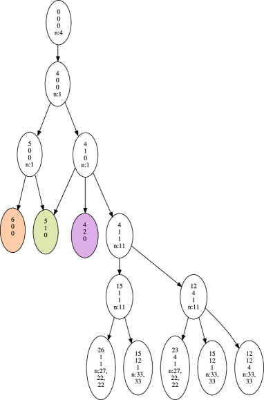
Figure 1: The beginning moves of the $45/33$ lower bound, scaled so that $T=33$ and $S=45$. The vertices contain the current loads of all three bins, and a string n: $i$ with $i$ being the next item presented by the Adversary. If there are several numbers after n:, the items are presented in the given order, regardless of packing by the player Algorithm. The coloured vertices are expanded in later figures.

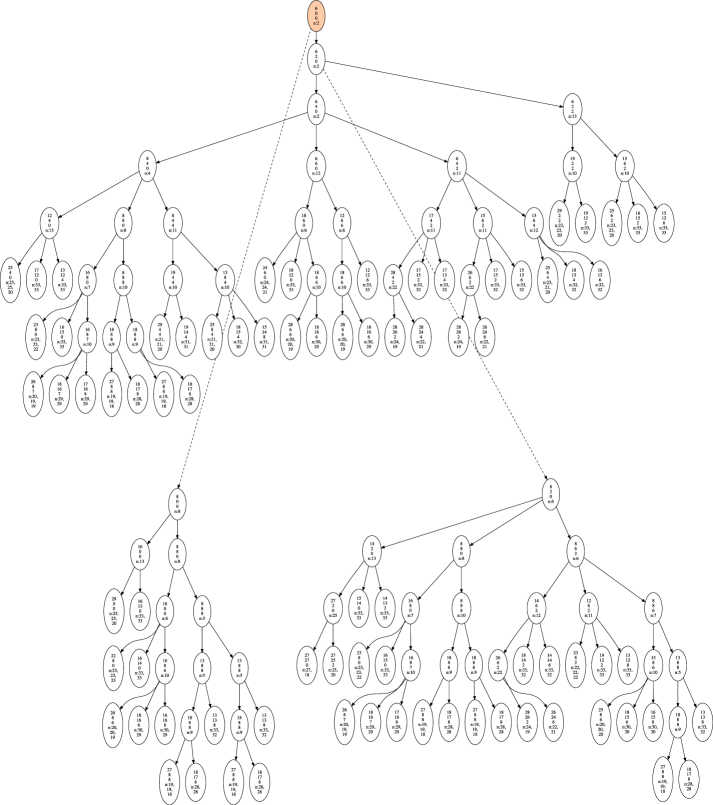
Figure 2: Game tree for the lower bound of $45/33$, starting with the bin configuration $(6,0,0,\{4,1,1\})$.

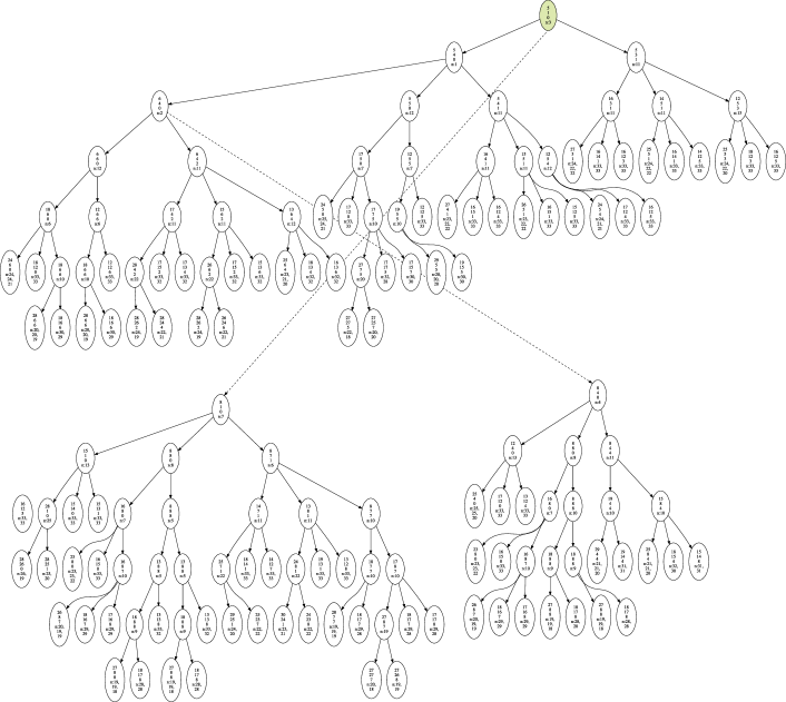
Figure 3: Game tree for the lower bound of $45/33$, starting with the bin configuration $(5,1,0,\{4,1,1\})$.

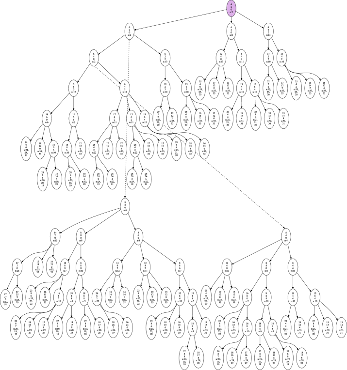
Figure 4: Game tree for the lower bound of $45/33$, starting with the bin configuration $(4,2,0,\{4,1,1\})$.

References

- [1] S. Albers and M. Hellwig. Semi-online scheduling revisited. Theor. Comput. Sci., 443:1–9, 2012.
- [2] J. Aspnes, Y. Azar, A. Fiat, S. Plotkin, and O. Waarts. On-line load balancing with applications to machine scheduling and virtual circuit routing. J. ACM, 44:486–504, 1997.
- [3] Y. Azar and O. Regev. On-line bin-stretching. In Randomization and Approximation Techniques in Computer Science, pages 71–81. Springer, 1998.
- [4] Y. Azar and O. Regev. On-line bin-stretching. Theor. Comput. Sci. 268(1):17–41, 2001.
- [5] P. Berman, M. Charikar, and M. Karpinski. On-line load balancing for related machines. J. Algorithms, 35:108–121, 2000.
- [6] M. Böhm. Lower Bounds for Online Bin Stretching with Several Bins. Student Research Forum Papers and Posters at SOFSEM 2016, CEUR WP Vol-1548, 2016.
- [7] M. Böhm, J. Sgall, R. van Stee, and P. Veselý. Better algorithms for online bin stretching. In Approximation and Online Algorithms (pp. 23-34). Springer International Publishing, 2014.
- [8] M. Böhm, J. Sgall, R. van Stee, and P. Veselý. The Best Two-Phase Algorithm for Bin Stretching. ArXiv preprint arXiv:1601.08111, 2016.
- [9] E. Coffman Jr., J. Csirik, G. Galambos, S. Martello, and D. Vigo. Bin Packing Approximation Algorithms: Survey and Classification, In P. M. Pardalos, D.-Z. Du, and R. L. Graham, editors, Handbook of Combinatorial Optimization, pages 455–531. Springer New York, 2013.
- [10] T. Ebenlendr, W. Jawor, and J. Sgall. Preemptive online scheduling: Optimal algorithms for all speeds. Algorithmica, 53:504–522, 2009.
- [11] M. Gabay, N. Brauner, V. Kotov. Computing lower bounds for semi-online optimization problems: Application to the bin stretching problem. HAL preprint hal-00921663, version 2, 2013.
- [12] M. Gabay, N. Brauner, V. Kotov. Improved Lower Bounds for the Online Bin Stretching Problem. HAL preprint hal-00921663, version 3, 2015.
- [13] M. Gabay, V. Kotov, N. Brauner. Semi-online bin stretching with bunch techniques. HAL preprint hal-00869858, 2013.
- [14] R. L. Graham. Bounds on multiprocessing timing anomalies. SIAM J. Appl. Math., 17:263–269, 1969.
- [15] D. Johnson. Near-optimal Bin Packing Algorithms. Massachusetts Institute of Technology, project MAC. Massachusetts Institute of Technology, 1973.
- [16] H. Kellerer and V. Kotov. An efficient algorithm for bin stretching. Operations Research Letters, 41(4):343–346, 2013.
- [17] H. Kellerer, V. Kotov, M. G. Speranza, and Z. Tuza. Semi on-line algorithms for the partition problem. Oper. Res. Lett., 21:235–242, 1997.
- [18] J. Ullman. The Performance of a Memory Allocation Algorithm. Technical Report 100, 1971.
- [19] Zobrist, Albert L. A new hashing method with application for game playing. ICCA journal 13.2: 69-73. 1970.