A posteriori error analysis for nonconforming approximation of multiple eigenvalues

Abstract.

In this paper we study an a posteriori error indicator introduced in E. Dari, R.G. Durán, C. Padra, Appl. Numer. Math., 2012, for the approximation of the Laplace eigenvalue problem with Crouzeix–Raviart non-conforming finite elements. In particular, we show that the estimator is robust also in presence of eigenvalues of multiplicity greater than one. Some numerical examples confirm the theory and illustrate the convergence of an adaptive algorithm when dealing with multiple eigenvalues.

1. Introduction

Although the a posteriori error analysis for eigenvalue problems arising from partial differential equations is a mature field of research, some intriguing questions remain open when discussing the convergence of an adaptive scheme for the approximation of eigenvalues with multiplicity greater than one.

In this paper we consider the approximation of Laplace eigenvalue by standard Crouzeix–Raviart finite elements (see [5] and, for instance, [3]). In [7] an a posteriori error indicator has been proposed for this problem and its efficiency and reliability have been proved. The analysis of [7] showed that the indicator is equivalent to the energy norm of the error in the eigenfunctions (up to higher order terms) and that it provides an upper bound for the error in the first eigenvalue (up to higher order terms). In this paper we are mainly interested in the case when an eigenvalue may have multiplicity greater than one. This topic has been the object of little research and only very recently people started investigating the issues originating from the presence of multiple eigenvalues (see, in particular, [2, 15, 11, 6, 9]).

The presented results contain a theoretical part, included in Sections 3 and 4, and some numerical experiments reported in Section 5.

In Section 3 we study the error estimates for the eigenfunctions and, recalling the results of [7], we show that the results extend in a natural way to the case of multiple eigenvalues. In Section 4, using some special tools adapted from [13], we extend the estimates for the eigenvalues to the general case of multiplicity $q\geq 1$. One of the main difficulties comes from the fact that, when using non-conforming finite elements, one cannot deduce from the min-max lemma that the discrete eigenvalues should be upper bounds of the corresponding continuous ones. In our analysis we study separately the cases when an eigenvalue is approximated by $q$ discrete eigenvalues from above or from below. Our analysis does not apply to the case when a continuous eigenvalue corresponds to discrete eigenvalues which can approximate it simultaneously from above or from below. It should however be noted that in most situations Crouzeix-Raviart element provides lower bound: this has been proved asymptotically for singular eigenspaces (see [1] and [7]). See also [4] where this property has been used for the construction of guaranteed lower bounds for eigenvalue approximation. Known examples of discrete eigenvalues which provide approximation from above are rare and computed on very coarse meshes.

The numerical results shown in Section 5 confirm the theory and aim at investigating the behavior of an adaptive procedure based on the studied indicator in case of multiple eigenvalues. As expected, it turns out that a correct procedure should take into account all discrete eigenfunctions approximating the same eigenspace (see [15]). One of the main issues raised by this investigation is that in general it is not known a priori (besides very particular situations like the one considered in our tests) the multiplicity of an eigenvalue of the continuous problem and it is not obvious to detect which discrete values correspond to it. This phenomenon requires further investigation and will be the object of future study.

2. Setting of the problem

Let $\Omega\subset\mathbb{R}^{d}$, $d=2,3$ be a polygonal or polyhedral Lipschitz domain, we consider the Laplacian eigenproblem: find $\lambda\in\mathbb{R}$ and $u\in H^{1}_{0}(\Omega)$ with $u\neq 0$ such that

(1) $$a(u,v)=\lambda(u,v)\quad\forall v\in H^{1}_{0}(\Omega),$$

where

$$a(u,v)=\int_{\Omega}\nabla u\nabla v\,dx\qquad(u,v)=\int_{\Omega}uv\,dx.$$

It is well known that the eigenvalues of the problem above form an increasing sequence tending to infinity:

(2) $$0<\lambda_{1}\leq\lambda_{2}\leq\dots\leq\lambda_{i}\leq\cdots$$

We denote by $u_{i}$ an eigenfunction associated to the eigenvalue $\lambda_{i}$; it is well known that the eigenfunctions can be chosen such that the following properties are satisfied:

(3) $$(u_{i},u_{i})=1\qquad (u_{i},u_{j})=0\quad\text{if }i\neq j$$

$$a(u_{i},u_{i})=\lambda_{i}\qquad a(u_{i},u_{j})=0\quad\text{if }i\neq j.$$

Let us introduce the Crouzeix–Raviart non conforming finite element space we shall work with (see [5]). We consider a regular family of decompositions of $\Omega$ into closed triangles or tetrahedra. Let $h_{K}$ denote the diameter of the element $K$ and $h=\max_{K\in\mathcal{T}}h_{K}$. The set of all faces $F$ of elements in $\mathcal{T}_{h}$ is denoted by $\mathcal{F}_{h}$. For any internal face $F$ let $K$ and $K^{\prime}$ be two elements such that $K\cap K^{\prime}=F$, we denote by $[v]_{F}$ the jump across $F$ for $v\in L^{2}(K\cup K^{\prime})$. For a face $F\subset\partial\Omega$ we set $[v]_{F}=v$. Then we define

$$V_{h}^{nc}=\{v\in L^{2}(\Omega):\ v|_{K}\in\mathcal{P}_{1}(K)\ \forall K\in\mathcal{T}_{h}\text{ and }\int_{F}[v]_{F}=0\ \forall F\in\mathcal{F}_{h}\}.$$

We introduce the following discrete bilinear form defined on $V_{h}^{nc}\times V_{h}^{nc}$

$$a_{h}(u,v)=\sum_{K\in\mathcal{T}_{h}}{\int_{K}}\nabla u\nabla v\,dx=\int_{\Omega}\nabla_{h}u\nabla_{h}v\,dx\qquad\forall u,v\in V_{h}^{nc}$$

where

$$\nabla_{h}u|_{{K}}=\nabla(u|_{{K}}).$$

Let us recall some standard notation. We set $\|\cdot\|^{2}_{0}=(\cdot,\cdot)$, the $L^{2}$-norm, and

(4) $$\|u\|_{1}^{2}=a(u,u)=\|\nabla u\|^{2}_{0} \forall u\in H^{1}_{0}(\Omega)$$

$$\|u\|^{2}_{h}=a_{h}(u,u)=\|\nabla_{h}u\|^{2}_{0} \forall u\in V_{h}^{nc}$$

Notice that thanks to the Poincaré inequality and to its discrete version for non conforming elements (see [10]) both $\|\cdot\|_{1}$ and $\|\cdot\|_{h}$ are norms on $H^{1}_{0}(\Omega)$ and $V_{h}^{nc}$, respectively.

Let $\tilde{V}=H^{1}_{0}(\Omega)+V_{h}^{nc}$, that is any element $\tilde{u}$ of $\tilde{V}$ can be written as the sum $\tilde{u}=u+u_{h}$ with $u\in H^{1}_{0}(\Omega)$ and $u_{h}\in V_{h}^{nc}$. We have that $\|\cdot\|_{h}$ is a norm in $\tilde{V}$ and that in the case of $u\in H^{1}_{0}(\Omega)$ it holds $\|u\|_{h}=\|u\|_{1}$.

Then the discrete eigenproblem reads: find $\lambda_{h}\in\mathbb{R}$ and $u_{h}\in V_{h}^{nc}$ with $u_{h}\neq 0$ such that

(5) $$a_{h}(u_{h},v)=\lambda_{h}(u_{h},v)\qquad\forall v\in V_{h}^{nc}.$$

Problem (5) admits exactly $N_{h}=\dim(V_{h}^{nc})$ positive eigenvalues with

(6) $$0<\lambda_{1,h}\leq\lambda_{2,h}\leq\dots\leq\lambda_{N_{h},h}.$$

Moreover, we denote by $u_{i,h}$ a discrete eigenfunction associated to the eigenvalue $\lambda_{i,h}$ with the following properties:

(7) $$(u_{i,h},u_{i,h})=1\qquad (u_{i,h},u_{j,h})=0\quad\text{if }i\neq j$$

$$a_{h}(u_{i,h},u_{i,h})=\lambda_{i,h}\qquad a_{h}(u_{i,h},u_{j,h})=0\quad\text{if }i\neq j.$$

We indicate with $E_{i,\dots,j}\subset H^{1}_{0}(\Omega)$ (resp. $E_{i,\dots,j,h}\subset V_{h}^{nc}$) the span of the eigenvectors $\{u_{i},\dots,u_{j}\}$ (resp. $\{u_{i,h},\dots,u_{j,h}\}$) and $P_{i,\dots,j}$ (resp. $P_{i,\dots,j,h}$) the elliptic projection onto $E_{i,\dots,j}$ (resp. $E_{i,\dots,j,h}$), that is

(8) $$\text{for }u\in H^{1}_{0}(\Omega),\ P_{i,\dots,j}u\in E_{i,\dots,j}\ \text{ s.t. }a(u-P_{i,\dots,j}u,v)=0 \forall v\in E_{i,\dots,j}$$

$$\text{for }u\in\tilde{V},\ P_{i,\dots,j,h}u\in E_{i,\dots,j,h}\ \text{ s.t. }a_{h}(u-P_{i,\dots,j,h}u,v)=0 \forall v\in E_{i,\dots,j,h}.$$

The discrete solution operator $T_{h}:L^{2}(\Omega)\to L^{2}(\Omega)$ is defined as $T_{h}f\in V_{h}^{nc}$ with

(9) $$a_{h}(T_{h}f,v)=(f,v)\quad\forall v\in V_{h}^{nc}.$$

In our a posteriori error analysis we shall also make use of the space of conforming piecewise linear elements

$$V_{h}^{c}=\{v\in H^{1}_{0}(\Omega):v|_{K}\in\mathcal{P}_{1}(K)\ \forall K\in\mathcal{T}_{h}\}.$$

The conforming discretization of the eigenvalue problem under consideration reads: find $\lambda^{c}_{h}\in\mathbb{R}$ and $u^{c}_{h}\in V_{h}^{c}$ with $u^{c}_{h}\neq 0$ such that

(10) $$a(u^{c}_{h},v)=\lambda^{c}_{h}(u^{c}_{h},v)\qquad v\in V_{h}^{c}.$$

Problem (10) admits $N^{c}_{h}=\dim(V_{h}^{c})$ positive eigenvalues

(11) $$0<\lambda^{c}_{1,h}\leq\lambda^{c}_{2,h}\leq\dots\leq\lambda^{c}_{N^{c}_{h},h}.$$

As in the case of non conforming discretization we denote by $u^{c}_{i,h}$ the eigenfunction associated to the eigenvalue $\lambda^{c}_{i,h}$ such that $(u^{c}_{i,h},u^{c}_{i,h})=1$ with the following orthogonality properties:

(12) $$(u^{c}_{i,h},u^{c}_{i,h})=1\qquad (u^{c}_{i,h},u^{c}_{j,h})=0\quad\text{if }i\neq j$$

$$a_{h}(u^{c}_{i,h},u^{c}_{i,h})=\lambda^{c}_{i,h}\qquad a_{h}(u^{c}_{i,h},u^{c}_{j,h})=0\quad\text{if }i\neq j.$$

Notice that $V_{h}^{c}=H^{1}_{0}(\Omega)\cap V_{h}^{nc}$, hence $N^{c}_{h}<N_{h}$ and $\lambda_{i.h}\leq\lambda^{c}_{i,h}$ for $i=1,\dots,N^{c}_{h}$ because of the min max characterization.

Let $P^{c}_{h}$ be the elliptic projection from $\tilde{V}$ onto $V_{h}^{c}$, that is: for all $u\in\tilde{V}$, $P^{c}_{h}u\in V_{h}^{c}$ such that

(13) $$a(P^{c}_{h}u,v)=a_{h}(u,v)\quad\forall v\in V_{h}^{c}.$$

Similarly to the nonconforming approximation, we denote by $E^{c}_{i,\dots,j,h}\subset V_{h}^{c}$ the span of the eigenvectors $\{u^{c}_{i,h},\dots,u^{c}_{j,h}\}$ and by $P^{c}_{i,\dots,j,h}$ the elliptic projection onto $E^{c}_{i,\dots,j,h}$, that is: for all $u\in\tilde{V}$, $P^{c}_{i,\dots,j,h}u\in E^{c}_{i,\dots,j,h}$ such that

(14) $$a_{h}(u-P^{c}_{i,\dots,j,h}u,v)=0\qquad\forall v\in E^{c}_{i,\dots,j,h}.$$

We shall make use of the Rayleigh quotient associated to the eigenvalue problem (1)

(15) $$\mathcal{R}(w)=\frac{a(w,w)}{(w,w)}\quad\forall w\in H^{1}_{0}(\Omega)\setminus\{0\}$$

and of the analogous quotient associated to the nonconforming discretization

(16) $$\mathcal{R}_{h}(w)=\frac{a_{h}(w,w)}{(w,w)}\quad\forall w\in V_{h}^{nc}\setminus\{0\}$$

In case of multiple eigenvalues we shall need to estimate the distance between eigenspaces associated to them and to their discrete counterpart. Let $E$ and $F$ be two subspaces of $\tilde{V}$, then the distance between them is defined as

$$\delta_{h}(E,F)=\sup_{\genfrac{}{}{0.0pt}{}{u\in E}{\|u\|_{h}=1}}\inf_{v\in F}\|u-v\|_{h}.$$

For nonzero functions $u$ and $v$, if $E=\mathop{\rm span}\nolimits\{u\}$, we write ${\delta_{h}}(u,F)$ instead of ${\delta_{h}}(E,F)$ and if $E=\mathop{\rm span}\nolimits\{u\}$ and $F=\mathop{\rm span}\nolimits\{v\}$, we write ${\delta_{h}}(u,v)$ for ${\delta_{h}}(E,F)$. We have $0\leq\delta_{h}(E,F)\leq 1$ and $\delta_{h}(E,F)=0$ if and only if $E\subseteq F$. If $\dim E=\dim F<\infty$ then $\delta_{h}(E,F)=\delta_{h}(F,E)$. If $P$ and $Q$ are the orthogonal projections onto $E$ and $F$, respectively, then $\delta_{h}(E,F)$ equals the largest singular value of the operator $(I-Q)P$ and

(17) $$\delta_{h}(E,F)=\|(I-Q)P\|_{\mathcal{L}(\tilde{V})},$$

where the notation $\|\cdot\|_{\mathcal{L}(\tilde{V})}$, as usual, denotes the operator norm from $\tilde{V}$ into itself. See for example [14] for these results and the characterization of the distance between subspaces.

3. Error estimates for the eigenfunctions

In this section we introduce the error indicators and present the a posteriori error estimates for the eigenfunctions.

First of all let us recall some properties of the Couzeix–Raviart space. Given $w\in H^{1}_{0}(\Omega)$, we denote by $w_{I}\in V_{h}^{nc}$ its edge/face average interpolant such that

(18) $$\int_{F}w_{I}=\int_{F}w\qquad\forall F\in\mathcal{F}_{h}.$$

It is well known that $\nabla_{h}w_{I}$ is the $L^{2}$-projection of $\nabla w$ onto the piecewise constant vector fields and that the following estimates hold true

(19) $$\|\nabla_{h}w_{I}\|_{0}\leq\|\nabla w\|_{0},$$

$$\|w-w_{I}\|_{L^{2}(K)}\leq C_{1}h_{K}\|\nabla w\|_{L^{2}(K)}.$$

Our error indicators make use of the following conforming postprocessing for the elements in $V_{h}^{nc}$. To any element $v\in V_{h}^{nc}$ we associate an element $\tilde{v}\in V_{h}^{c}$ obtained by averaging the value of $v$ at the vertices of the triangulation $\mathcal{T}_{h}$. Namely, following [7], for each internal vertex ${\mathsf{P}}$ we consider all elements $K_{i}\in\mathcal{T}_{h}$ for $i=1,\dots,M$ which share the vertex $P$ and define

(20) $$\tilde{v}({\mathsf{P}})=\sum_{i=1}^{M}w_{i}v|_{K_{i}}({\mathsf{P}}),$$

where $w_{i}$ are suitable weights such that $\sum_{i=1}^{M}w_{i}=1$.

Lemma 1.

The following estimates hold true with constants $C$ independent of $h$

(21) $$\|\tilde{v}\|_{0}\leq C\|v\|_{0}$$

$$\|\nabla\tilde{v}\|_{0}\leq C\|\nabla_{h}v\|_{0}$$

$$\|\tilde{v}-v\|_{0}\leq Ch\|\nabla_{h}(\tilde{v}-v)\|_{0}.$$

Proof.

Let ${\mathsf{P}}$ be a vertex of the mesh. It is proved in [7, Th. 5.2], that for all $w\in H^{1}_{0}(\Omega)$

(22) $$|\tilde{v}({\mathsf{P}})-v|_{K}({\mathsf{P}})|\leq\frac{C}{h_{K}^{d/2-1}}\|\nabla_{h}(v-w)\|_{L^{2}(\Omega_{\mathsf{P}})},$$

where $\Omega_{\mathsf{P}}$ is the union of elements $K$ containing ${\mathsf{P}}$.

For $w=0$, using an inverse estimate, we also have

$$|\tilde{v}({\mathsf{P}})-v|_{K}({\mathsf{P}})|\leq\frac{C}{h_{K}^{d/2}}\|v\|_{L^{2}(\Omega_{\mathsf{P}})},$$

Then, for an element $K$ we write, using the standard notation $N_{i}$ for nodal basis functions,

$$\tilde{v}-v=\sum_{i=1}^{d+1}\left(\tilde{v}({\mathsf{P}}_{i})-v|_{K}({\mathsf{P}}_{i})\right)N_{i}$$

and

$$\nabla(\tilde{v}-v)=\sum_{i=1}^{d+1}\left(\tilde{v}({\mathsf{P}}_{i})-v|_{K}({\mathsf{P}}_{i})\right)\nabla N_{i}$$

and therefore, if $\tilde{K}$ is the union of neighbors of $K$, using the above estimates and standard estimates for the basis functions $N_{i}$, we obtain

$$\|\tilde{v}-v\|_{0,K}\leq C\|v\|_{0,\tilde{K}}$$

and

$$\|\nabla(\tilde{v}-v)\|_{0,K}\leq C\|\nabla_{h}v\|_{0,\tilde{K}}.$$

Then the triangle inequality yields the first two estimates in (21). The last one can also be easily obtained from (22) taking into account that $\|N_{i}\|_{0}\leq Ch_{K}^{d/2}$ and choosing $w=\tilde{v}$.

∎

We define the local and global error estimators as follows

(23) $$\mu^{2}_{i,{K}}=\|\nabla\tilde{u}_{i,h}-\nabla_{h}u_{i,h}\|^{2}_{L^{2}({K})},\quad \mu^{2}_{i}=\sum_{K}\mu^{2}_{i,{K}}$$

$$\eta^{2}_{i,{K}}=h_{K}^{2}\|\lambda_{i,h}u_{i,h}\|_{L^{2}({K})}^{2}, \eta^{2}_{i}=\sum_{K}\eta^{2}_{i,{K}}.$$

The following theorem gives the error estimates for the eigenfunctions in term of the above error indicators.

Theorem 2.

Let $\lambda_{i}$ be an eigenvalue of (1) with multiplicity $q\geq 1$ (that is $\lambda_{i}=\dots=\lambda_{i+q-1}$) and let $E_{i,\dots,i+q-1}$ be the associated eigenspace. Assume that $\lambda_{j,h}$ is a discrete eigenvalue of (5) converging to $\lambda_{i}$ and that $E_{j,h}$ is the associated eigenspace ($j=i,\dots,i+q-1$). Then

(24) $${\delta_{h}}(E_{j,h},E_{i,\dots,i+q-1})\leq{\delta_{h}}(E_{j,h},H^{1}_{0}(\Omega))+C_{1}\frac{\eta_{j}}{\lambda_{j,h}}+h.o.t.$$

More precisely, we have

$$|h.o.t.|\leq\frac{C_{\Omega}}{\lambda_{j,h}}\left((\lambda_{i}-\lambda_{j,h})+(\lambda_{i}\lambda_{j,h})^{1/2}\inf_{v\in E_{i,\dots,i+q-1}}\|v-u_{j,h}\|_{L^{2}(\Omega)}\right),$$

where $C_{1}$ is the constant in (19) and $C_{\Omega}$ is the Poincaré constant.

Proof.

The proof is based on that of [7, Th. 3.2]. Here we make more precise the case of multiple eigenvalues.

Let us fix $j=i,\dots,i+q-1$ and let us consider the eigensolution $(\lambda_{j,h},u_{j,h})$ of (5); we recall that $\|u_{j,h}\|_{0}=1$. Let $u_{j}(h)\in E_{i,\dots,i+q-1}$ be such that $\|u_{j}(h)\|_{0}=1$ and

(25) $$\|u_{j}(h)-u_{j,h}\|_{h}=\inf_{v\in E_{i,\dots,i+q-1}}\|v-u_{j,h}\|_{h}.$$

We observe that $u_{j}(h)$ is an eigenfunction associated to the multiple eigenvalue $\lambda_{i}$, hence it satisfies (1). Then applying the same argument as in the proof of [7, Th. 3.2], we have that

(26) $$\|u_{j}(h)-u_{j,h}\|_{h}\leq \inf_{v\in H^{1}_{0}(\Omega)}\|v-u_{j,h}\|_{h}+C_{1}\eta+C_{\Omega}\Big{(}(\lambda_{i}-\lambda_{j,h})$$

$$+(\lambda_{i}\lambda_{j,h})^{1/2}\|u_{j}(h)-u_{j,h}\|_{0}\Big{)}.$$

From the definition of the gap we have to estimate

$${\delta_{h}}(E_{j,h},E_{i,\dots,i+q-1})=\sup_{\genfrac{}{}{0.0pt}{}{u\in E_{j,h}}{\|u\|_{h}=1}}\inf_{v\in E_{i,\dots,i+q-1}}\|u-v\|_{h}=\inf_{v\in E_{i,\dots,i+q-1}}\Big{\|}\frac{u_{j,h}}{\|u_{j,h}\|_{h}}-v\Big{\|}_{h},$$

since $E_{j,h}$ is generated by $u_{j,h}$. With a simple computation, using the above estimate for the eigenfunction $u_{j,h}$ and the fact that $\|u_{j,h}\|_{h}=\lambda_{j,h}$, we obtain the desired bound. ∎

It remains to estimate the gap between $E_{j,h}$ and $H^{1}_{0}(\Omega)$ in terms of our indicators.

Lemma 3.

Under the same assumptions as in Theorem 2, the following estimate holds true:

(27) $${\delta_{h}}(E_{j,h},H^{1}_{0}(\Omega))\leq\frac{1}{\lambda_{j,h}}\mu_{j}.$$

Proof.

By definition we have

$${\delta_{h}}(E_{j,h},H^{1}_{0}(\Omega)) =\sup_{\genfrac{}{}{0.0pt}{}{u\in E_{j,h}}{\|u\|_{h}=1}}\inf_{v\in H^{1}_{0}(\Omega)}\|u-v\|_{h}$$

$$=\frac{1}{\lambda_{j,h}}\inf_{v\in H^{1}_{0}(\Omega)}\|u_{j,h}-v\|_{h}$$

$$\leq\frac{1}{\lambda_{j,h}}\|u_{j,h}-\tilde{u}_{j,h}\|_{h}=\frac{1}{\lambda_{j,h}}\mu_{j}.$$

∎

For the efficiency of these error estimators we refer to [7] where the following local bounds from below of the error are proved.

Theorem 4.

Let $\lambda_{i}$ be an eigenvalue of (1) with multiplicity $q\geq 1$ and let $\lambda_{j,h}$ be a discrete eigenvalue converging to $\lambda_{i}$ ($j=i,\dots,i+q-1$). Let $u_{j}(h)\in E_{i,\dots,i+q-1}$ be such that (25) holds true. Then there exist constants $C$ depending only on the regularity of the elements such that for all elements $K\in\mathcal{T}_{h}$ it holds

$$\mu_{K}\leq C\|\nabla_{h}(u_{j}(h)-u_{j,h})\|_{L^{2}(K^{*})}$$

$$\eta_{K}\leq C\|\nabla_{h}(u_{j}(h)-u_{j,h})\|_{L^{2}(K)}+h.o.t.,$$

where $K^{*}$ is the union of all the elements in $\mathcal{T}_{h}$ sharing a vertex with $K$ and

$$h.o.t.=h_{K}\|\lambda_{i}u_{j}(h)-\lambda_{j,h}u_{j,h}\|_{L^{2}(K)}.$$

4. Error estimates for the eigenvalues

In this section we prove error estimates for the eigenvalues using the a posteriori error indicators introduced in (23). In the case of conforming approximation of the eigenvalue problem (1) it is well known that each discrete eigenvalue is greater than or equal to the corresponding continuous one. In the case of nonconforming discretization this is not true in general. In [1, 7] it is proved that, for singular eigenfunctions, the Crouzeix-Raviart approximation provides asymptotic lower bounds of the corresponding eigenvalue. For this reason, in our analysis we consider separately the cases where a multiple eigenvalue is approximated by below or by above. More precisely, given a multiple eigenvalue $\lambda_{i}$ of multiplicity $q\geq 1$, we assume that either $\lambda_{j,h}\leq\lambda_{i}$ or $\lambda_{i}\leq\lambda_{j,h}$ for all $j=i,\dots,i+q-1$.

Let us consider first the case when the eigenvalues are approximated from below.

The first theorem gives an estimate of the relative error for the eigenvalues in terms of the norm of the distance of the discrete eigenspace from the subspace of conforming finite elements orthogonal to the span of the first $i$ conforming eigenfunctions.

Theorem 5.

Let $\lambda_{i}$ be an eigenvalue with multiplicity $q$ so that

$$\lambda_{i-1}<\lambda_{i}=\dots=\lambda_{i+q-1}<\lambda_{i+q},$$

and let $\lambda_{i,h}\leq\dots\leq\lambda_{i+q-1,h}$ be the $q$ discrete eigenvalues converging to $\lambda_{i}$. We assume that $\lambda_{j,h}\leq\lambda_{i}$ for $j=i,\dots,i+q-1$. Then

(28) $$\frac{\lambda_{i}-\lambda_{j,h}}{\lambda_{i}}\leq\|(I-P^{c}_{h}+P^{c}_{1,\dots,i-1,h})P_{i,\dots,j,h}\|^{2}_{\mathcal{L}(\tilde{V})}.$$

Proof.

We observe that the discretization by conforming finite elements produces $q$ discrete eigenvalues converging to $\lambda_{i}$ and that it holds $\lambda_{i}\leq\lambda^{c}_{j,h}$ for $j=i,\dots,i+q-1$.

Let us fix $j$ with $i\leq j\leq i+q-1$, then by assumption we have

$$\lambda_{j,h}\leq\lambda_{i}\leq\lambda^{c}_{j,h}.$$

The operators $I-P^{c}_{h}+P^{c}_{1,\dots,i-1,h}$ and $P_{i,\dots,j,h}$ are orthogonal projections with respect to the norm $\|\cdot\|_{h}$ of $\tilde{V}$. Therefore $\|(I-P^{c}_{h}+P^{c}_{1,\dots,i-1,h})P_{i,\dots,j,h}\|_{\mathcal{L}(\tilde{V})}\leq 1$ (see [12, Th. 6.34, p. 56]). If $\|(I-P^{c}_{h}+P^{c}_{1,\dots,i-1,h})P_{i,\dots,j,h}\|_{\mathcal{L}(\tilde{V})}=1$ then the bound (28) is obviously true, since $\lambda_{j,h}\leq\lambda_{i}$. Hence we assume that

$$\|(I-P^{c}_{h}+P^{c}_{1,\dots,i-1,h})P_{i,\dots,j,h}\|_{\mathcal{L}(\tilde{V})}<1.$$

Thanks to [12, Th. 3.6, Chap. I] this inequality implies that

$$\dim((P^{c}_{h}-P^{c}_{1,\dots,i-1,h})E_{i,\dots,j,h})=\dim(E_{i,\dots,j,h})=j-i+1.$$

We choose $\overline{u}\in(P^{c}_{h}-P^{c}_{1,\dots,i-1,h})E_{i,\dots,j,h}\subset V_{h}^{c}$ such that $\|\overline{u}\|_{h}=\|\overline{u}\|_{{1}}=1$ and

$$\mathcal{R}(\overline{u})=\max_{\genfrac{}{}{0.0pt}{}{w\in(P^{c}_{h}-P^{c}_{1,\dots,i-1,h})E_{i,\dots,j,h}}{w\neq 0}}\mathcal{R}(w),$$

where $\mathcal{R}(w)$ is the Rayleigh quotient defined in (15).

Let us consider the following orthogonal decomposition of $\overline{u}$ in $\tilde{V}$:

$$\overline{u}=u+v\quad\text{with }u\in E_{1,\dots,j,h}\text{ and }v\in(E_{1,\dots,j,h})^{\perp},$$

that is $a_{h}(w,v)=0$ for all $w\in E_{1,\dots,j,h}$. Notice that since $u\in V_{h}^{nc}$ also $v\in V_{h}^{nc}$. We have that

$$\|v\|_{h} =\delta_{h}(\overline{u},E_{1,\dots,j,h}) \text{by definition of }v$$

$$\leq\delta_{h}((P^{c}_{h}-P^{c}_{1,\dots,i-1,h})E_{i,\dots,j,h},E_{1,\dots,j,h}) \overline{u}\in(P^{c}_{h}-P^{c}_{1,\dots,i-1,h})E_{i,\dots,j,h}$$

$$\leq\delta_{h}((P^{c}_{h}-P^{c}_{1,\dots,i-1,h})E_{i,\dots,j,h},E_{i,\dots,j,h})$$ the inf is taken on a smaller subset

$$=\|(I-P^{c}_{h}+P^{c}_{1,\dots,i-1,h})P_{i,\dots,j,h}\|_{\mathcal{L}(\tilde{V})}$$ this is a characterization of the gap.

We now prove that

$$0\leq\frac{\lambda^{c}_{j,h}-\lambda_{j,h}}{\lambda^{c}_{j,h}}\leq\|v\|_{h}$$

$$0\leq\frac{\lambda_{i}-\lambda_{j,h}}{\lambda_{i}}\leq\|v\|_{h}.$$

We observe that the first inequality implies the second one.
By definition of $\overline{u}$ and the min-max principle for the eigenvalues we have that

$$\lambda^{c}_{j,h}\leq\mathcal{R}(\overline{u}).$$

Moreover, since $u\in E_{1,\dots,j,h}$, we have that $u=\sum_{s=1}^{j}\alpha_{s}u_{s,h}$ and

$$\mathcal{R}_{h}(u)=\frac{a_{h}(u,u)}{(u,u)}=\frac{\sum_{s=1}^{j}\alpha_{s}^{2}a_{h}(u_{s,h},u_{s,h})}{\sum_{s=1}^{j}\alpha_{s}^{2}(u_{s,h},u_{s,h})}=\frac{\sum_{s=1}^{j}\alpha_{s}^{2}\lambda_{s,h}}{\sum_{s=1}^{j}\alpha_{s}^{2}}\leq\lambda_{j,h}.$$

In conclusion, the following inequalities hold true ($i\leq j\leq i+q-1$):

$$\mathcal{R}_{h}(u)\leq\lambda_{j,h}\leq\lambda_{j}\leq\lambda^{c}_{j,h}\leq\mathcal{R}(\overline{u}),$$

and the rest of the proof is based on a bound for $1/\mathcal{R}_{h}(u)-1/\mathcal{R}(\overline{u})$.

Since $v\in(E_{1,\dots,j,h})^{\perp}$ we have that $a_{h}(u,v)=0$. We want to show that also $(u,v)=0$. Since we know that $v\in V_{h}^{nc}$ and that $E_{1,\dots,j,h}$ is invariant with respect to $T_{h}$, we have also $a_{h}(T_{h}u,v)=0$. Hence

$$0=a_{h}(T_{h}u,v)=(u,v),$$

due to the definition of $T_{h}$.

We now compute

$$\frac{1}{\mathcal{R}_{h}(u)} -\frac{1}{\mathcal{R}(\overline{u})}=\frac{(u,u)}{a_{h}(u,u)}-\frac{(u,u)+(v,v)}{a_{h}(u,u)+a_{h}(v,v)}$$

$$=\frac{a_{h}(u,u)(u,u)+a_{h}(v,v)(u,u)-a_{h}(u,u)(u,u)-{a_{h}}(u,u)(v,v)}{a_{h}(u,u)\left(a_{h}(u,u)+a_{h}(v,v)\right)}$$

$$=\frac{1}{a_{h}(u,u)+a_{h}(v,v)}\left(\frac{a_{h}(v,v)}{a_{h}(u,u)}\left((u,u)+(v,v)\right)-\left(\frac{a_{h}(v,v)}{a_{h}(u,u)}+1\right)(v,v)\right)$$

$$=\left(\frac{1}{\mathcal{R}(\overline{u})}-\frac{1}{\mathcal{R}_{h}(v)}\right)\frac{a_{h}(v,v)}{a_{h}(u,u)}$$

$$\leq\frac{1}{\mathcal{R}(\overline{u})}\frac{a_{h}(v,v)}{a_{h}(u,u)}\leq\frac{1}{\lambda_{j}}\frac{a_{h}(v,v)}{a_{h}(u,u)}.$$

We get

$$\frac{1}{\lambda_{jh}}-\frac{1}{\lambda_{j}}\leq\frac{1}{\mathcal{R}_{h}(u)}-\frac{1}{\mathcal{R}(\overline{u})}\leq\frac{1}{\lambda_{j}}\frac{a_{h}(v,v)}{a_{h}(u,u)}$$

from which we obtain

$$\frac{\lambda_{j}}{\lambda_{j,h}}\leq 1+\frac{a_{h}(v,v)}{a_{h}(u,u)}=\frac{{a_{h}}(u,u)+a_{h}(v,v)}{a_{h}(u,u)}=\frac{1}{a_{h}(u,u)}$$

and then

$$\frac{\lambda_{j}-\lambda_{j,h}}{\lambda_{j}}=1-\frac{\lambda_{j,h}}{\lambda_{j}}\leq 1-a_{h}(u,u)=a_{h}(v,v)=\|v\|_{h}^{2}.$$

We can obtain also

$$\frac{\lambda^{c}_{j,h}-\lambda_{j,h}}{\lambda^{c}_{j,h}}\leq a_{h}(v,v)=\|v\|_{h}^{2},$$

by using the following inequality

$$\frac{1}{\lambda_{j,h}}-\frac{1}{\lambda^{c}_{j,h}}\leq\frac{1}{\mathcal{R}_{h}(u)}-\frac{1}{\mathcal{R}(\overline{u})}\leq\frac{1}{\lambda^{c}_{j,h}}\frac{a_{h}(v,v)}{a_{h}(u,u)}.$$

∎

We now want to estimate the right hand side of (28) in terms of $P^{c}_{h}$ and $P_{i,\dots,j,h}$ only.

First of all, we observe that

$$\|(I-P^{c}_{h}+P^{c}_{1,\dots,i-1,h})P_{i,\dots,j,h}\|^{2}_{\mathcal{L}(\tilde{V})}=\|(I-P^{c}_{h})P_{i,\dots,j,h}\|^{2}_{\mathcal{L}(\tilde{V})}+\|P^{c}_{1,\dots,i-1,h}P_{i,\dots,j,h}\|^{2}_{\mathcal{L}(\tilde{V})};$$

hence it remains to estimate the second term, which represents the projection of the nonconforming invariant subspace associated to the eigenvalues numbered from $i$ to $j$ onto the subspace of conforming invariant subspace generated by the first $i-1$ eigenvalues.

Proposition 6.

Let $\lambda_{i}$ be an eigenvalue with multiplicity $q$, so that

$$\lambda_{i-1}<\lambda_{i}=\dots=\lambda_{i+q-1}<\lambda_{i+q},$$

and let $\lambda_{i,h}\leq\dots\leq\lambda_{i+q-1,h}$ be the $q$ discrete eigenvalues converging to $\lambda_{i}$. We assume that $\lambda^{c}_{i-1,h}<\lambda_{i,h}$ then, for $h$ small enough, there exists $\beta>0$ such that

(29) $$\|P^{c}_{1,\dots,i-1,h}P_{i,\dots,j,h}\|_{\mathcal{L}(\tilde{V})}\leq\frac{\|(I-P^{c}_{h})T_{h}P^{c}_{1,\dots,i-1,h}\|_{\mathcal{L}(\tilde{V})}}{{\beta}}\|(I-P^{c}_{h})P_{i,\dots,j,h}\|_{\mathcal{L}(\tilde{V})}$$

where $T_{h}$ is the solution operator defined in (9).

Proof.

Using the same notation as in [13, Th. 4.2], we introduce the following operators:

$$P=P_{i,\dots,j,h},\quad\tilde{R}=P^{c}_{1,\dots,i-1,h},$$

so that $P$ is the elliptic projection onto the invariant nonconforming subspace $E_{i,\dots,j,h}$, and $\tilde{R}$ is the elliptic projection onto the invariant conforming subspace $E^{c}_{1,\dots,i-1,h}$, that is

$$\tilde{R}=P^{c}_{1,\dots,i-1,h}:\tilde{V}\to E^{c}_{1,\dots,i-1,h}$$

$$a(\tilde{R}w,v)=a_{h}(w,v)\quad\forall v\in E^{c}_{1,\dots,i-1,h}.$$

We observe that $\|\tilde{R}w\|_{1}\leq\|w\|_{h}$

Moreover, the spectrum of $(\tilde{R}T_{h}\tilde{R})|_{\mathrm{Im}\tilde{R}}$ is equal to $\{1/\lambda^{c}_{1,h},\dots,1/\lambda^{c}_{i-1,h}\}$. Indeed, $\mathrm{Im}\tilde{R}$ is the span of $\{u^{c}_{1,h},\dots,u^{c}_{i-1,h}\}$ and by definition $T_{h}u^{c}_{k,h}$ ($1\leq k\leq i-1$) belongs to $V_{h}^{nc}$ and is given by

$$a_{h}(T_{h}u^{c}_{k,h},v)=(u^{c}_{k,h},v)\quad\forall v\in V_{h}^{nc}.$$

Hence, $\tilde{R}T_{h}u^{c}_{k,h}$ belongs to $E^{c}_{1,\dots,i-1,h}$ and satisfies

$$a(\tilde{R}T_{h}u^{c}_{k,h},v)=a_{h}(T_{h}u^{c}_{k,h},v)=(u^{c}_{k,h},v)\quad\forall v\in E^{c}_{1,\dots,i-1,h}.$$

It follows that

$$\tilde{R}T_{h}u^{c}_{k,h}=\frac{1}{\lambda^{c}_{k,h}}u^{c}_{k,h},$$

so that $1/\lambda^{c}_{k,h}$ ($1\leq k\leq i-1$) coincides with the spectrum of $(\tilde{R}T_{h}\tilde{R})|_{\mathrm{Im}\tilde{R}}$ (there cannot be other eigenvalues, since the dimension of $\mathrm{Im}\tilde{R}$ is equal to $i-1$).

Since the spectrum of $(\tilde{R}T_{h}\tilde{R})|_{\mathrm{Im}\tilde{R}}$ does not contain the eigenvalues ${\nu}_{j,h}=1/\lambda_{j,h}$ for $j=i,\dots,i+q-1$, the operator $\tilde{R}(T_{h}-{\nu}_{j,h})\tilde{R}$ has a bounded inverse and

$$d\|\tilde{R}P\|_{\mathcal{L}(\tilde{V})}\leq\|\tilde{R}(T_{h}-{\nu}_{j,h})\tilde{R}P\|_{\mathcal{L}(\tilde{V})},$$

where

$$d=\min_{k=1,\dots,i-1}|{\nu}^{c}_{k,h}-{\nu}_{j,h}|=|{\nu}^{c}_{i-1,h}-{\nu}_{j,h}|{\,\geq\,}|{\nu}^{c}_{i-1,h}-{\nu}_{i,h}|=\frac{\lambda_{i,h}-\lambda^{c}_{i-1,h}}{\lambda_{i,h}\lambda^{c}_{i-1,h}}.$$

We have that

(30) $$\tilde{R}(T_{h}-{\nu}_{j,h})\tilde{R}P=\tilde{R}(T_{h}-{\nu}_{j,h})P^{c}_{h}P.$$

Namely, since $\tilde{R}\tilde{R}P=\tilde{R}P^{c}_{h}P$, it is enough to show that $\tilde{R}T_{h}\tilde{R}P=\tilde{R}T_{h}P^{c}_{h}P$. We have that $T^{c}_{h}=P^{c}_{h}T_{h}$, which implies that $\tilde{R}T_{h}\tilde{R}P=\tilde{R}T^{c}_{h}\tilde{R}P$ and that $\tilde{R}T_{h}P^{c}_{h}P=\tilde{R}T^{c}_{h}P^{c}_{h}P$. Hence, we only have to show that $\tilde{R}T^{c}_{h}\tilde{R}P=\tilde{R}T^{c}_{h}P^{c}_{h}P$. Indeed, it holds $\tilde{R}T^{c}_{h}\tilde{R}=\tilde{R}T^{c}_{h}P^{c}_{h}$. In order to show this result, let’s take $f\in V_{h}^{nc}$, then $P^{c}_{h}f=\sum_{i=1}^{\dim V_{h}^{c}}\alpha_{i}u^{c}_{i,h}$ and $\tilde{R}f=\sum_{i\in I}\alpha_{i}u^{c}_{i,h}$, where $I$ is the finite set of indices corresponding to the range of $\tilde{R}$. The equality (30) is then easily obtained by comparing $\tilde{R}T^{c}_{h}\tilde{R}f$ and $\tilde{R}T^{c}_{h}P^{c}_{h}f$ and taking into account that $u_{i,h}^{c}$ are eigenfunctions of $T^{c}_{h}$.

From (30) we obtain

$$\tilde{R}(T_{h}-{\nu}_{j,h})P^{c}_{h}P =\tilde{R}T_{h}P^{c}_{h}P-\tilde{R}T_{h}P+\tilde{R}T_{h}P-\tilde{R}{\nu}_{j,h}P^{c}_{h}P$$

$$=-\tilde{R}T_{h}(I-P^{c}_{h})P+\tilde{R}(T_{h}-{\nu}_{j,h})P+{\nu}_{j,h}\tilde{R}(I-P^{c}_{h})P.$$

The last term is equal to zero since $\tilde{R}=\tilde{R}P^{c}_{h}$. Hence

$$d\|\tilde{R}P\|_{\mathcal{L}(\tilde{V})} \leq\|\tilde{R}T_{h}(I-P^{c}_{h})P\|_{\mathcal{L}(\tilde{V})}+\|\tilde{R}(T_{h}-{\nu}_{j,h})P\|_{\mathcal{L}(\tilde{V})}$$

$$\leq\|\tilde{R}T_{h}(I-P^{c}_{h})\|_{\mathcal{L}(\tilde{V})}\|(I-P^{c}_{h})P\|_{\mathcal{L}(\tilde{V})}+\|\tilde{R}P\|_{\mathcal{L}(\tilde{V})}\|P(T_{h}-{\nu}_{j,h})P\|_{\mathcal{L}(\tilde{V})}$$

$$\leq\|(I-P^{c}_{h})T_{h}\tilde{R}\|_{\mathcal{L}(\tilde{V})}\|(I-P^{c}_{h})P\|_{\mathcal{L}(\tilde{V})}+\delta\|\tilde{R}P\|_{\mathcal{L}(\tilde{V})},$$

where $\delta$ is given by

$${\delta=\|P(T_{h}-{\nu}_{j,h})P\|_{\mathcal{L}(\tilde{V})}.}$$

Since $P$ is the elliptic projection onto the invariant nonconforming subspace $E_{i,\dots,j,h}$ we have that

$$\delta\leq|{\nu}_{i+q-1,h}-{\nu}_{i,h}|=\frac{1}{\lambda_{i,h}}-\frac{1}{\lambda_{i+q-1,h}}=\frac{\lambda_{i+q-1,h}-\lambda_{i,h}}{\lambda_{i,h}\lambda_{i+q-1,h}}\leq\frac{\lambda_{i+q-1,h}-\lambda_{i,h}}{\lambda_{i,h}\lambda^{c}_{i-1,h}}.$$

For $h$ small enough, ${\beta=d-\delta}>0$ and we conclude that

$$\|\tilde{R}P\|_{\mathcal{L}(\tilde{V})}\leq\frac{\|(I-P^{c}_{h})T_{h}\tilde{R}\|_{\mathcal{L}(\tilde{V})}}{{\beta}}\|(I-P^{c}_{h})P\|_{\mathcal{L}(\tilde{V})}.$$

∎

Combining the results of Theorem 5 and of Proposition 6 we have the following result

(31) $$\frac{\lambda_{i}-\lambda_{j,h}}{\lambda_{i}}\leq\left(1+\frac{\|(I-P^{c}_{h})T_{h}P^{c}_{1,\dots,i-1,h}\|_{\mathcal{L}(\tilde{V})}}{{\beta}}\right)\|(I-P^{c}_{h})P_{i,\dots,j,h}\|^{2}_{\mathcal{L}(\tilde{V})},$$

from which we deduce the following a posteriori estimate involving the indicators introduced in (23)

Theorem 7.

Let us assume the same hypotheses as in Theorem 5 and Proposition 6. Then, for $h$ small enough, we have

$$\frac{\lambda_{i}-\lambda_{j,h}}{\lambda_{i}}\leq C{\delta_{h}^{2}}(E_{i,\dots,j,h},V_{h}^{c})\leq C\sum_{k=i}^{j}\frac{1}{\lambda^{2}_{k,h}}\mu_{k}^{2}.$$

Proof.

The quotient within the parentheses in (31) tends to zero as $h$ tends to zero, hence it is bounded. On the other hand, from (17) we have that

$$\|(I-P^{c}_{h})P_{i,\dots,j,h}\|^{2}_{\mathcal{L}(\tilde{V})}={\delta_{h}^{2}}(E_{i,\dots,j,h},V_{h}^{c}).$$

Thanks to (7), $u_{k,h}$ for $k=i,\dots,j$ form an orthogonal basis for $E_{i,\dots,j,h}$, so that (see, e.g. [13, Cor. 2.2])

$${\delta_{h}^{2}}(E_{i,\dots,j,h},V_{h}^{c})\leq\sum_{k=i}^{j}{\delta_{h}^{2}}(E_{k,h},V_{h}^{c}).$$

Applying Lemma 3 we arrive at the desired estimate. ∎

Let us now consider the case of discrete nonconforming eigenvalues approximating the continuous ones from above. We estimate first the distance between an eigenvalue $\lambda_{i}$ of multiplicity $q$ and the average of the discrete eigenvalues $\lambda_{k,h}$ for $k=i,\dots,j$ (here $j=i,\dots,i+q-1$).

Lemma 8.

Let $\lambda_{i}$ be an eigenvalue with multiplicity $q$, so that

$$\lambda_{i-1}<\lambda_{i}=\dots=\lambda_{i+q-1}<\lambda_{i+q},$$

and let $\lambda_{i,h}\leq\dots\leq\lambda_{i+q-1,h}$ be $q$ discrete eigenvalues converging to $\lambda_{i}$. We assume that $\lambda_{j,h}\geq\lambda_{i}$ for $j=i,\dots,i+q-1$, then for all $j=i,\dots,i+q-1$

(32) $$\frac{1}{J}\sum_{k=i}^{j}\lambda_{k,h}-\lambda_{i}\leq\frac{1}{J}\sum_{k=i}^{j}\left(6\mu_{k}^{2}+4C_{1}\eta_{k}^{2}+4|h.o.t.|^{2}\right)+|h.o.t.|_{2}$$

where

$$|h.o.t.|_{2}=\frac{C}{J}\sum_{k=i}^{j}\sum_{m=1}^{k-i}h^{2m}\sum_{l=i}^{k-m}C(\mu_{k}+\mu_{l})^{2}\lambda_{l,h},$$

$J=j-i+1$ and the higher order terms $|h.o.t.|$ are defined in Th. 2.

Proof.

The proof is divided into two parts. We start by estimating the error for the first discrete eigenvalue $\lambda_{i,h}$ converging to $\lambda_{i}$, next we shall deal with the general case.

First case. Let $\lambda_{i}$ with $i\geq 1$ be a multiple eigenvalue with multiplicity $q\geq 1$.

It holds that $\lambda_{i}\leq\lambda_{i,h}\leq\lambda^{c}_{i,h}$. The first inequality holds by assumption and the second one is due to the min-max principle for the eigenvalues and the fact that $V_{h}^{c}\subset V_{h}^{nc}$. Let $u_{i,h}\in V_{h}$ be the eigensolution associated with $\lambda_{i,h}$ and $u_{i}(h)\in E_{i,\dots,i+q-1}$ be such that $\|u_{i}(h)\|_{0}=1$ and satisfies (25) and (26), then, for all $v\in(P^{c}_{h}-P^{c}_{1,\dots,i-1,h})E_{i,h}$ with $\|v\|_{0}=1$, we have

$$\lambda_{i}+\lambda_{i,h}\leq\|\nabla u_{i}(h)\|^{2}_{0}+\mathcal{R}(v)=\|\nabla u_{i}(h)\|^{2}_{0}+\|\nabla v\|^{2}_{0}.$$

Hence

$$\lambda_{i}+\lambda_{i,h} \leq\|\nabla u_{i}(h)\|^{2}_{0}+\|\nabla v\|^{2}_{0}$$

$$=\|\nabla(u_{i}(h)-v)\|^{2}_{0}+2\int_{\Omega}\nabla u_{i}(h)\nabla v\,dx$$

$$=\|\nabla(u_{i}(h)-v)\|^{2}_{0}+2\lambda_{i}\int_{\Omega}u_{i}(h)v\,dx$$

$$=\|\nabla(u_{i}(h)-v)\|^{2}_{0}-\lambda_{i}\|u_{i}(h)-v\|^{2}_{0}+2\lambda_{i}$$

and

$$\lambda_{i,h}-\lambda_{i}\leq\|\nabla(u_{i}(h)-v)\|^{2}_{0}\leq 2\|\nabla_{h}(u_{i}(h)-u_{i,h})\|^{2}_{0}+2\|\nabla_{h}(u_{i,h}-v)\|^{2}_{0}.$$

The first term on the right hand side can be estimated with (26). Since $v$ is arbitrary in $(P^{c}_{h}-P^{c}_{1,\dots,i-1,h})E_{i,h}$, we can set $v=(P^{c}_{h}-P^{c}_{1,\dots,i-1,h})u_{i,h}$. Hence

$$\|\nabla_{h}(u_{i,h}-v)\|_{0} =\|\nabla_{h}(u_{i,h}-(P^{c}_{h}-P^{c}_{1,\dots,i-1,h})u_{i,h})\|_{0}$$

$$\leq\|\nabla_{h}(I-P^{c}_{h})u_{i,h}\|_{0}+\|\nabla_{h}P^{c}_{1,\dots,i-1,h}u_{i,h}\|_{0}.$$

The hypotheses of Proposition 6 are satisfied, so that

$$\|\nabla_{h}(u_{i,h}-v)\|_{0}\leq C\|\nabla_{h}(I-P^{c}_{h})u_{i,h}\|_{0}\leq C\mu_{i}.$$

Finally, we obtain

$$\lambda_{i,h}-\lambda_{i}\leq 4\mu_{i}^{2}+C_{1}\eta_{i}^{2}+|h.o.t.|^{2}.$$

Second case. Due to the min-max characterization for the eigenvalues we have that for $k=i,\dots,j$

$$\lambda_{i}\leq\lambda_{k,h}\leq\lambda^{c}_{k,h}.$$

Let us take $J$ arbitrary elements $v_{1},\dots,v_{J}$ of $V_{h}^{c}$ belonging to $(E_{1,\dots,i-1,h}^{c})^{\perp}$ (to be specified later in the proof) which are orthogonal to each other, that is $(v_{l},v_{m})=0$ for $l\neq m$.

We show that

(33) $$\sum_{k=i}^{j}\lambda^{c}_{k,h}\leq\sum_{l=1}^{J}\mathcal{R}(v_{l}),$$

where $\mathcal{R}(v_{l})$ denotes the Rayleigh quotient (see (15)). For simplicity, we show the result under the normalization $\|v_{l}\|_{0}=1$ ($l=1,\dots,J$), so that $\mathcal{R}(v_{l})=a(v_{l},v_{l})$ (this does not limit the generality of our proof). Let us write $v_{l}$ by decomposing it as its components in $E^{c}_{i,\dots,j,h}$ and a remainder as follows:

$$v_{l}=\sum_{k=i}^{j}\alpha_{lk}u^{c}_{k,h}+w_{l}.$$

It turns out that

$$\mathcal{R}(v_{l})=a(v_{l},v_{l})\geq\sum_{k=i}^{j}\alpha_{lk}^{2}\lambda^{c}_{k,h}+\left(1-\sum_{k=i}^{j}\alpha_{lk}^{2}\right)\lambda^{c}_{j+1,h},$$

so that

$$\sum_{l=1}^{J}\mathcal{R}(v_{l})\geq\sum_{k=i}^{j}\lambda^{c}_{k,h}+\sum_{k=i}^{j}(\lambda^{c}_{j+1,h}-\lambda^{c}_{k,h})\left(1-\sum_{l=1}^{J}\alpha_{lk}^{2}\right).$$

Hence, the estimate (33) is proved if we can show that

$$\sum_{l=1}^{J}\alpha_{lk}^{2}\leq 1\quad\forall k.$$

This follows from the orthogonality of the $v_{l}$’s. Indeed, for all $k$,

$$\sum_{l=1}^{J}\alpha_{lk}^{2}=\Big{(}\sum_{l=1}^{J}\alpha_{lk}v_{l},u^{c}_{k,h}\Big{)}\leq\Big{\|}\sum_{l=1}^{J}\alpha_{lk}v_{l}\Big{\|}_{0}=\sqrt{\sum_{l=1}^{J}\alpha_{lk}^{2}}.$$

As in the proof of the first case, for $k=i,\dots,j$, let $u_{k}(h)\in E_{i,\dots,i+q-1}$ with $\|u_{k}(h)\|_{0}=1$ be such that (26) holds true. Then we have

$$J\lambda_{i}+\sum_{k=i}^{j}\lambda_{k,h} \leq\sum_{k=i}^{j}\left(\|\nabla u_{k}(h)\|^{2}_{0}+\|\nabla v_{k-i+1}\|^{2}_{0}\right)$$

$$=\sum_{k=i}^{j}\left(\|\nabla(u_{k}(h)-v_{k-i+1})\|^{2}_{0}-\lambda_{i}\|u_{k}(h)-v_{k-i+1}\|^{2}_{0}\right)+2J\lambda_{i}$$

Hence

(34) $$\frac{1}{J}\sum_{k=i}^{j}\lambda_{k,h}-\lambda_{i} \leq\frac{1}{J}\sum_{k=i}^{j}\|\nabla(u_{k}(h)-v_{k-i+1})\|^{2}_{0}$$

$$\leq\frac{2}{J}\sum_{k=i}^{j}\left(\|\nabla_{h}(u_{k}(h)-u_{k,h})\|^{2}_{0}+\|\nabla_{h}(u_{k,h}-v_{k-i+1})\|^{2}_{0}\right)$$

The first term in the sum appearing in the last line of (34) can be bounded by (26), while for the remaining term we now make a choice for the definition of $v_{l}$, $l=1,\dots,J$, which will be analogous to what has been done in the first case.

For $k=i,\dots,j$ let $\hat{u}_{k,h}\in V_{h}^{c}$ be the projection of $u_{k,h}$ onto $(E^{c}_{1,\dots,i-1,h})^{\perp}$ performed according to (13).

Then we choose

(35) $$v_{1}={\hat{u}_{i,h}}$$

$$v_{l}={\hat{u}_{i+l-1,h}}-\sum_{m=1}^{l-1}\frac{({\hat{u}_{i+l-1,h}},v_{m})}{\|v_{m}\|^{2}_{0}}v_{m},\qquad l=2,\dots,J.$$

By construction, we have that for $h$ small enough

(36) $$\frac{1}{2}\leq\|v_{l}\|_{0}\leq C.$$

The same argument used in the first case shows that

(37) $$\|\nabla_{h}(u_{k,h}-\hat{u}_{k,h})\|^{2}_{0}\leq C\mu^{2}_{k},\quad\forall k=i,\dots,j.$$

Moreover, standard properties of the projections and a duality argument give

(38) $$\|u_{k,h}-\hat{u}_{k,h}\|_{0}\leq Ch\mu_{k},\quad\forall k=i,\dots,j.$$

In order to estimate the right hand side of (34), we start with $j=i$; we have

(39) $$\|\nabla v_{1}\|^{2}_{0}=\|\nabla\hat{u}_{i,h}\|^{2}_{0}\leq\|\nabla_{h}u_{i,h}\|^{2}_{0}=\lambda_{i,h}.$$

For $k=i+1,\dots,j$, set $l=k-i+1$, so that we have

(40) $$\|\nabla_{h}(u_{k,h}-v_{l})\|^{2}_{0}\leq\|\nabla_{h}(u_{k,h}-{\hat{u}_{k,h}})\|^{2}_{0}+\sum_{m=1}^{l-1}\frac{|({\hat{u}_{k,h}},v_{m})|^{2}}{\|v_{m}\|_{0}^{4}}\|\nabla v_{m}\|_{0}^{2}.$$

We detail the cases when $k=i+1$ and $k=i+2$; the general situation should then be clear.

If $k=i+1$, then $l=2$, so that the last term in (40) can be estimated using (36) and (38) as follows:

(41) $$|({\hat{u}_{i+1,h}},v_{1})| \leq|({\hat{u}_{i+1,h}}-u_{i+1,h},v_{1})|+|(u_{i+1,h},v_{1}-u_{i,h})|$$

$$\leq\|{\hat{u}_{i+1,h}}-u_{i+1,h}\|_{0}\|v_{1}\|_{0}+\|u_{i+1,h}\|_{0}\|{\hat{u}_{i,h}}-u_{i,h}\|_{0}$$

$$\leq Ch(\mu_{i+1}+\mu_{i}).$$

Hence we obtain

$$\|\nabla_{h}(u_{i+1,h}-v_{2})\|^{2}_{0} \leq\|\nabla_{h}(u_{i+1,h}-{\hat{u}_{i+1,h}})\|^{2}_{0}+Ch^{2}(\mu_{i+1}^{2}+\mu_{i}^{2})\lambda_{i,h}$$

$${\,\leq C}\mu_{i+1}^{2}+Ch^{2}(\mu_{i+1}^{2}+\mu_{i}^{2})\lambda_{i,h}$$

and

(42) $$\|\nabla v_{2}\|^{2}_{0}\leq 2\|\nabla{\hat{u}_{i+1,h}}\|^{2}_{0}+2\frac{|({\hat{u}_{i+1,h}},v_{1})|^{2}}{\|v_{1}\|_{0}^{4}}\|\nabla v_{1}\|^{2}_{0}\leq C\lambda_{i+1,h}+Ch^{2}(\mu_{i+1}+\mu_{i})^{2}\lambda_{i,h}.$$

If $k=i+2$, then $l=3$ and we have two terms in the sum on the right hand side of (40), that is $({\hat{u}_{i+2,h}},v_{1})$ and $({\hat{u}_{i+2,h}},v_{2})$. For the first term, working as in (41), we obtain

(43) $$|({\hat{u}_{i+2,h}},v_{1})| \leq C\|{\hat{u}_{i+2,h}}-u_{i+2,h}\|_{0}\|v_{1}\|_{0}+\|u_{i+2,h}\|_{0}\|{\hat{u}_{i,h}}-u_{i,h}\|_{0}$$

$$\leq Ch(\mu_{i+2}+\mu_{i}).$$

Next, from the definition of $v_{1}$ and $v_{2}$ we have using also (41)

(44) $$|({\hat{u}_{i+2,h}},v_{2})| \leq|({\hat{u}_{i+2,h}}-u_{i+2,h},v_{2})|+|(u_{i+2,h},{\hat{u}_{i+1,h}}-u_{i+1,h})|$$

$$\quad+\frac{|({\hat{u}_{i+1,h}},v_{1})|}{\|v_{1}\|^{2}_{0}}|(u_{i+2,h},{\hat{u}_{i,h}}-u_{i,h})|$$

$$\leq Ch(\mu_{i+2}+\mu_{i+1})+Ch^{2}(\mu_{i+1}+\mu_{i})\mu_{i}.$$

Therefore, putting things together, we get

$$\|\nabla_{h}(u_{i+2,h}-v_{3})\|^{2}_{0}\leq\mu_{i+2}^{2}+Ch^{2}\sum_{l=i}^{i+1}(\mu_{i+2}+\mu_{l})^{2}\lambda_{l,h}+Ch^{4}(\mu_{i+1}+\mu_{i})^{2}\mu_{i}^{2}\lambda_{i+1,h}.$$

From this estimate it is straightforward to obtain the estimate of $\|\nabla v_{3}\|_{0}$, and so on. ∎

It is now easy to obtain the desired a posteriori error estimate for the eigenvalues approaching the continuous one from above.

Theorem 9.

Under the same hypotheses as in Lemma 8 the following bound holds true for $j=i,\dots,i+q-1$

$$\frac{\lambda_{j,h}-\lambda_{i}}{\lambda_{i}}\leq\frac{1}{\lambda_{i}}\left(\frac{1}{J}\sum_{k=i}^{j}\left(6\mu_{k}^{2}+4C_{1}\eta_{k}^{2}+4|h.o.t.|^{2}\right)+|h.o.t.|_{2}+\frac{1}{J}\sum_{k=i}^{j-1}(\lambda_{j,h}-\lambda_{k,h})\right).$$

Proof.

The proof is straightforward since

$$\lambda_{j,h}-\lambda_{i}=\frac{1}{J}\sum_{k=i}^{j-1}\left(\lambda_{j,h}-\lambda_{k,h}\right)+\frac{1}{J}\sum_{k=i}^{j}\lambda_{k,h}-\lambda_{i},$$

which combined with (32) gives the result.

∎

5. Numerical results

In this section we present some numerical results obtained applying the estimator discussed in this paper.

The aim of our tests is not to show the reliability and the efficiency of the error indicator, since results in this direction have been already reported in [7]. The emphasis of our computations will be put on the approximation of multiple eigenvalues. There are few papers concerning adaptivity for the numerical approximation of multiple eigenvalues, among those we recall in particular [15], [6], and [9]. A consequence of the results contained in these three papers is, in particular, that an adaptive algorithm aiming at a refinement procedure for the approximation of a multiple eigenvalue, needs to take into account indicators belonging to all the discrete eigenfunctions approximating the continuous eigenspace.

In all our numerical tests the discrete eigenvalues are lower bounds for the continuous ones. Actually, we checked the first one hundred eigenvalues of our numerical tests and all of them appear to be lower bounds for the corresponding exact frequencies. Our experience, is that the method generally provides eigenvalues converging from below (apart from very pathological examples with few elements). So far, a proof of this fact is still missing.

We focus our attention on eigenvalues of multiplicity two. We consider an adaptive algorithm based on standard Dörfler marking strategy [8]. In case of double eigenvalues, we choose either to mark elements according to the error indicator based on one of the two discrete corresponding eigenfunctions, or to the sum of the indicators of the two eigenfunctions. From the discussion of the results we are going to present, it will be clear that the results of [15], [6], and [9] are confirmed. A more comprehensive and detailed study of the numerical tests will be included in a forthcoming paper.

5.1. The square ring domain

Let $\Omega$ be the domain obtaining by subtracting the square $(1/3,2/3)^{2}$ from the square $(0,1)^{2}$. This is the same domain considered in [15, Sect. 2].

It turns out that $\lambda_{2}$ is an eigenvalue with multiplicity two. More precisely, the two-dimensional eigenspace corresponding to $\lambda_{2}=\lambda_{3}$ can be generated by two singular eigenfunctions: each of them has a singularity at two opposite reentrant corners of $\Omega$. We used the reference value $\lambda_{2}=\lambda_{3}=84.517\dots$ computed by Aitken extrapolation using very fine meshes and conforming linear elements.

We use Matlab for our tests, so that the eigenvalues/eigenvectors are computed with the command eigs. At each stage we compute the three smallest eigenvalues and take into account the second and third ones.

We start by using a refinement strategy based on the discrete eigenfunction $u_{2,h}$ (notice that, due to the fact that the discrete eigenvalues are lower bounds, this corresponds to the one which is farther away from the double eigenvalue we want to approximate). The initial non-structured mesh is shown in Figure 1.

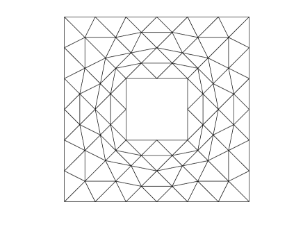
Figure 1. The initial mesh for the square ring test case

The plot of the discrete eigenvalues is reported in Figure 2.

Figure 2. The values of the discrete eigenvalues $\lambda_{2,h}$ and $\lambda_{3,h}$ on the square ring for different refinement levels (non structured initial mesh, refined based on $u_{2,h}$)

It is clear that the phenomenon already explained in [15] is present. The two discrete eigenvalues apparently change their position as the mesh is refined. For example, on the first mesh the two values are equal since the mesh is symmetric. It turns out that the solver determines a decomposition of the discrete eigenspace: let’s call $u_{j,h_{1}}$ ($j=2,3$) the two eigenfunctions on the initial mesh. The first refinement step is then performed by using the eigenfunction $u_{2,h_{1}}$; it happens that on the second mesh $\lambda_{2,h_{2}}$ and $\lambda_{3,h_{2}}$ are separated and correspond to new eigenfunctions $u_{2,h_{2}}$ and $u_{3,h_{2}}$. Actually, due to the performed refinement, this can be interpreted as if $u_{3,h_{2}}$ was an improved approximation of $u_{2,h_{1}}$; in some sense, the position of the two eigenfunctions has exchanged after the first refinement step. This phenomenon is more clear by looking at the corresponding meshes (see Figure 3): the second mesh has been refined at the North-West and South-East corners, while the new second eigenfunction $u_{2,h_{2}}$ is singular at the other two opposite corners.

Figure 3. The eigenfunctions corresponding to $\lambda_{2,h}$ on the square ring for the first four refinement levels (non structured initial mesh, refined based on $u_{2,h}$)

In order to better highlight this phenomenon, in Figure 4 we report a sequence of meshes obtained after eight level of refinements. It is clear that the method refines a region close to all four reentrant corners even if we are constructing our indicator only according to the second discrete eigenfunction. Moreover, the refinement strategy is not optimal since at each step only two of the four involved regions are considered.

Figure 4. Eight level of refinements of the square ring domain: indicator based on $u_{2,h}$

As a second test, we consider an adaptive strategy driven by the approximation of the eigenfunction $u_{3,h}$ corresponding to the third eigenvalue. A plot of the values of $\lambda_{2,h}$ and $\lambda_{3,h}$ is reported in Figure 5.

Figure 5. The values of the discrete eigenvalues $\lambda_{2,h}$ and $\lambda_{3,h}$ on the square ring for different refinement levels (non structured initial mesh, refined based on $u_{3,h}$)

It is clear that in this case the adaptive procedure is effective in pushing the convergence of $\lambda_{3,h}$, while $\lambda_{2,h}$ is converging more slowly.

The corresponding meshes are reported in Figure 6, where it can be seen that the refinements is always performed in a neighborhood of the same two corners.

Figure 6. Eight level of refinements of the square ring domain: indicator based on $u_{3,h}$

The eigenfunctions on the first four meshes are plotted in Figure 7: it can be seen that they always have singularities about the top right and bottom left reentrant corners. It should be clear that this behavior is just a good luck of this particular situation. Readers are warned that in case of invariant spaces of dimension greater than one, an effective adaptive strategy should consider all involved discrete eigenfunctions.

Figure 7. The eigenfunctions corresponding to $\lambda_{3,h}$ on the square ring for the first four refinement levels (non structured initial mesh, refined based on $u_{3,h}$)

This approach is presented as a conclusion of this section, where we repeat the same computation with an error indicator based on both singular eigenfunctions $u_{2,h}$ and $u_{3,h}$. The plot of the eigenvalues is reported in Figure 8 where it can be observed that now the two discrete values approximating the double eigenvalue $\lambda_{2}=\lambda_{3}$ are almost superimposed.

Figure 8. The values of the discrete eigenvalues $\lambda_{2,h}$ and $\lambda_{3,h}$ on the square ring for different refinement levels (non structured initial mesh, refined based on both $u_{2,h}$ and $u_{3,h}$)

For completeness, we report in Figure 9 the eigenfunctions corresponding to $\lambda_{2,h}$ and $\lambda_{3,h}$ after three refinements and in Figure 10 the sequence of mesh obtained after eight level of refinements.

Figure 9. Eigenfunctions corresponding to $\lambda_{2,h}$ and $\lambda_{3,h}$ after three levels of refinements: indicator based on $u_{2,h}$ and $u_{3,h}$

Figure 10. Eight level of refinements of the square ring domain: indicator based on $u_{2,h}$ and $u_{3,h}$

The convergence history of the adaptive algorithm is shown in Figure 11. It can be seen that the procedure is performing optimally with respect to the degrees of freedom. Finally, the effectivity index is reported in Figure 12; it can be seen that the ratio between the error in the eigenvalues and the indicators is bounded above and below.

(a) $\lambda_{2,h}$

(b) $\lambda_{3,h}$

Figure 11. Convergence history of the adaptive procedure: indicator based on $u_{2,h}$ and $u_{3,h}$

Figure 12. Effectivity index: indicator based on $u_{2,h}$ and $u_{3,h}$