Tolerating Silent Data Corruption in Opaque Preconditioners

Abstract

We demonstrate algorithm-based fault tolerance for silent, transient data corruption in “black-box” preconditioners. We consider both additive Schwarz domain decomposition with an ILU(k) subdomain solver, and algebraic multigrid, both implemented in the Trilinos library. We evaluate faults that corrupt preconditioner results in both single and multiple MPI ranks. We then analyze how our approach behaves when then application is scaled. Our technique is based on a Selective Reliability approach that performs most operations in an unreliable mode, with only a few operations performed reliably. We also investigate two responses to faults and discuss the performance overheads imposed by each. For a non-symmetric problem solved using GMRES and ILU, we show that at scale our fault tolerance approach incurs only 22% overhead for the worst case. With detection techniques, we are able to reduce this overhead to 1.8% in the worst case.

I Introduction

Recent studies indicate that large parallel computers will continue to become less reliable as energy constraints tighten, component counts increase, and manufacturing sizes decrease [1, 2, 3]. This unreliability may manifest in two different ways: either as “hard” faults, which cause the loss of one or more parallel processes, or as “soft” faults, which cause incorrect arithmetic or storage, but do not kill the running application. Large-scale systems today experience frequent process loss. Applications recover from it using global checkpoint / restart (C/R), with current research looking at optimizing the process through, e.g., multi-level checkpointing [4] or by using domain knowledge of algorithms to create checkpoint schemes that have lower overhead [5].

This paper focuses on soft faults. Specifically, we consider those that corrupt data or computations, without the hardware or system detecting them and notifying the application that a fault occurred. We call this type of soft fault Silent Data Corruption (SDC). SDC is much less frequent than process failures, but much more threatening, since the application may silently return an incorrect answer. In physical simulations, the wrong answer could have costly and even life-threatening consequences. Users’ trust in the results of numerical simulations can lead to disaster if those results are wrong, as for example in the 1991 collapse of the Sleipner A oil platform [6]. Unlike with hard faults, applications currently have few recovery strategies. Hardware detection without correction may cost nearly as much as full hardware correction. Hardware vendors can harden chips against soft faults, but doing so will increase chip complexity and likely either increase energy usage or decrease performance. An open field of research and the focus of this paper is designing algorithms that can tolerate SDC.

We present the following contributions:

• We show an algorithm-based fault tolerance approach for iterative linear solvers that enables the use of opaque preconditioners without algorithmic or code modifications.

• We demonstrate our approach for two different iterative solvers: the Conjugate Gradient method (CG) for symmetric positive definite matrices, and the Generalized Minimal Residual Method (GMRES) for nonsymmetric matrices. We do so for two preconditioners: additive Schwarz preconditioner with an ILU(k) subdomain solver, and algebraic multigrid (AMG).

• We relate the scale at which the problem is run to the overhead introduced by our fault tolerance approach.

• We present detection and rollback strategies that work with our fault-tolerance approach to reduce lost time due to SDC significantly.

Many engineering and scientific applications solve large sparse linear systems using iterative algorithms. Almost all of these solves use preconditioners. They may take time to set up, and will add to the time per iteration, but aim to save overall run time by reducing the total number of iterations. An important contribution of our work is that we treat preconditioners as opaque. That is, we do not need to modify the preconditioning algorithm or implementation. This matters because preconditioners are often orders of magnitude more complex than the iterative solvers that utilize them, in terms of both algorithms and lines of code. For example, one can express CG in a dozen lines of code, but the algebraic multigrid implementation MueLu [7] we use in this work includes over half a million lines of code from several Trilinos packages, as of the 11.8 Trilinos release, not counting third-party sparse direct factorization libraries for coarse-grid solves.

Prior work in algorithm-based fault tolerance for linear algebra problems focused on introducing checksums or other encoding schemes into the algorithm itself. One designs the algorithm to maintain a checksum relationship either while it is running, or after it completes [8, 9, 10, 11, 12]. This requires in-depth knowledge of the method and data structures, and requires modifying algorithms to incorporate fault detection and correction code. Even if this could be done for preconditioner algorithms as complicated as algebraic multigrid, adding checksums to an implementation would be impractical and error-prone, given the sheer amount of code to modify. Such a code would need to be rewritten from the ground up to use checksums.

Rather than attempt to rewrite every method to use an encoding scheme, we advocate a selective reliability approach [13, 14] that focuses fault tolerance effort on iterative solvers rather than preconditioners. The primary focus of this work is the use of preconditioners in linear solvers, where the preconditioner is assumed to be faulty. We consider the domain decomposition technique Additive Schwarz using an Incomplete LU factorization ILU(k), and a multi-level preconditioner Algebraic Multigrid. We also demonstrate that selective reliability can be used to create other fault-tolerant solvers besides the original “FT-GMRES” [13].

We also assess a concept presented by Elliott et al. [14] showing that enforcing bounded error is sufficient for iterative linear solvers. We consider the “Skeptical Programming” approach presented by Elliott et al. [14], and draw conclusions about the amalgamation of these approaches. The faults that motivate these fault tolerance approaches require scale to be observed. We conjecture that any approach has to consider the implications of both strong and weak scaling. Specifically, we evaluate a preconditioning strategy that runs at scale and keeps faults local, while also evaluating a preconditioning approach that may spread corruption to other processes as part preconditioning.

This paper is organized as follows:

1. In §II, we introduce the preconditioned linear solvers we evaluate.

2. In §III, we describe the types of preconditioners we chose and discuss how they propagate errors.

3. In §IV, we describe our fault injection methodology, and explain how we characterize faults.

4. In §V, we present findings that show the average number of extra preconditioner calls, given various types of faults.

5. In §VIII, we summarize results and discuss future work.

II Preconditioned Linear Solvers

We consider two solvers that are capable of solving different classes of problems. The Generalized Minimal Residual Method (GMRES) from Saad and Schultz [15] can solve nonsymmetric problems. The Method of Conjugate Gradients (CG) [16] can only solve symmetric positive definite (SPD) linear systems, but is faster for doing so. CG is used in the NAS Parallel Benchmarks [17] and in Mantevo miniapps like HPCCG [18].

Linear solvers often utilize preconditioners as a means to accelerate convergence. More specifically, preconditioning is a transformation that attempts to improve some aspect of the linear system, typically the condition number. We consider preconditioning in two different ways. Left preconditioning solves the preconditioned problem $M^{-1}(Ax-b)$, which requires a preconditioner application at the start of the solve. Right preconditioning solves $AM^{-1}Mx=b$, and requires a preconditioner application to also compute a solution update.

Algorithm 1 presents right-preconditioned GMRES. GMRES applies the preconditioner in lines 12 and 29. Note that the solution update (Line 29) need not be calculated every iteration, and is often not computed until the solver exits.

Algorithm 1 (Right-preconditioned) GMRES

1:Linear system $Ax=b$ and initial guess $x_{0}$

2:Approximate solution $x_{m}$ for some $m\geq 0$

3:

4:$r_{0}:=b-Ax_{0}$$\triangleright$ Unpreconditioned initial residual vector

5:

6:$\beta:=\|r_{0}\|_{2}$

7:

8:$q_{1}:=r_{0}/\beta$

9:

10:for $j=1,2,\dots$ until convergence do

11:

12:Solve $Mz_{j}=q_{j}$ for $z_{j}$$\triangleright$ Apply preconditioner

13:

14:$v_{j+1}:=Az_{j}$$\triangleright$ Apply the matrix $A$

15:

16:for $i=1,2,\dots,k$ do$\triangleright$ Orthogonalize

17:

18:$H(i,j):=q_{i}^{*}v_{j+1}$

19:

20:$v_{j+1}:=v_{j+1}-q_{i}H(i,j)$

21:end for

22:

23:$H(j+1,j):=\|v_{j+1}\|_{2}$

24:

25:$q_{j+1}:=v_{j+1}/H(j+1,j)$$\triangleright$ New basis vector

26:

27:$y_{j}:=\displaystyle\operatornamewithlimits{arg\,min}_{y}\|H(1:j+1,1:j)y-\beta e_{1}\|_{2}$

28:

29:$x_{j}:=x_{0}+M^{-1}[q_{1},q_{2},\dots,q_{j}]y_{j}$$\triangleright$ Solution update

30:end for

Algorithm 2 presents left-preconditioned CG. Preconditioner applications occur on Lines 6 and 18. Note that left-preconditioned CG does not require a preconditioner application to compute its solution update.

Algorithm 2 (Left-preconditioned) CG

1:Linear system $Ax=b$ and initial guess $x_{0}$

2:Approximate solution $x_{m}$ for some $m\geq 0$

3:

4:$r_{0}:=b-Ax_{0}$$\triangleright$ Unpreconditioned initial residual vector

5:

6:Solve $Mz_{0}=r_{0}$ for $z_{0}$$\triangleright$ Apply preconditioner

7:

8:$p_{0}:=z_{0}$

9:

10:for $j=1,2,\dots$ until convergence do

11:

12:$\alpha_{j}:=(r_{j},z_{j})/(Ap_{j},p_{j})$

13:

14:$x_{j+1}:=x_{j}+\alpha_{j}p_{j}$

15:

16:$r_{j+1}:=r_{j}-\alpha_{j}Ap_{j}$

17:

18:Solve $Mz_{j+1}=r_{j+1}$ for $z_{j+1}$$\triangleright$ Apply preconditioner

19:

20:$\beta_{j}:=(r_{j+1},z_{j+1})/(r_{j},z_{j})$

21:

22:$p_{j+1}:=z_{j+1}+\beta_{j}p_{j}$

23:end for

Our results center around observing the number of extra preconditioner applications relative to solving the problem without SDC. That is, we observe the impact of $\tilde{z}=M^{-1}w$, where $\tilde{z}$ indicates the corrupted output of a preconditioner call. In § III we give more details on on how we decompose problems across multiple processes, and in § IV we explain what $\tilde{z}$ looks like given faults on some (or all) parallel processes.

II-A Selective Reliability

Our fault-tolerance strategy rests on relating numerical methods that naturally correct errors to system-level fault tolerance. In particular, we assume a selective reliability or “sandboxing” programming model that lets algorithm developers isolate faults to certain parts of the algorithm in a coarse-grained way. Bridges et al. [13] used this idea to develop the fault-tolerant linear solver FT-GMRES. FT-GMRES uses a reliable “outer” solver, preconditioned by an unreliable “inner” solver. Any faults that occur in the inner solver manifest as a “different preconditioner” to the outer solver. The outer solver is chosen to be Flexible GMRES [19], which can tolerate a preconditioner that changes between iterations. The inner solver was chosen to be GMRES, though any linear solver would work. Nested solvers are a common idea in numerical algorithms; the authors applied this idea to fault tolerance by choosing the right outer solver and observing that inner solves could run unreliably. Selective reliability is a programming model that requires codesign between algorithms, system software, and hardware. Neither Bridges et al. [13] nor we attempt to implement this programming model; possible implementation strategies include redundancy or software error-correcting codes.

In this paper, we express FT-GMRES as FGmres->Gmres. This notation captures the outer solver FGmres and the inner solver Gmres. Should the inner solver uses a preconditioner, e.g., ILU, we then write FGmres->Gmres->ILU. The authors of FT-GMRES assumed that since GMRES is considered “robust” as a solver, it would makes sense to use FGmres->Gmres over combinations like FGmres->Cg. We evaluate this in § V.

II-B Implementation

We implemented our solvers using the Tpetra [20] sparse linear algebra package in the Trilinos framework [21] and validated them against both MATLAB and the solvers in Trilinos’ Belos package [22]. Implementing our solvers using Trilinos lets us benefit from the scalability and performance of its sparse matrices and dense vectors. In addition, basing our research in Trilinos also gives us access to a wealth of numerical algorithms, on which we elaborate in § III.

III Preconditioners

This paper shows how solvers behave in the presence of faulty preconditioners. Given that our solvers are parallel, we must consider parallel preconditioners. We examine two popular examples: single level additive Schwarz domain decomposition with no overlap, and Algebraic Multigrid (AMG). We have chosen preconditioners that utilize these decomposition techniques because each exhibits different types of communication patterns with respect to preconditioning.

III-A Additive Schwarz

Single-level additive Schwarz domain decomposition (see [23]) divides the solution vector into $k$ subdomains, either with or without overlap. Typical MPI implementations assign one subdomain to each MPI process. Each subdomain applies a solver (of any kind) locally. Additive Schwarz then “glues” the subdomains’ results back together to form the preconditioner’s output. We use Trilinos’ implementation in the Ifpack2 package to create our preconditioner, and choose Incomplete LU with zero fill, ILU(0) (see [19]), as our subdomain solver.

We use no overlap with additive Schwarz, because this means that any corruption in a subdomain will not impact output from other subdomains. That is, with zero overlap, there is no communication between subdomains after applying the local preconditioner. This differs from multigrid preconditioners.

III-B Algebraic Multigrid

Algebraic Multigrid (AMG) is a robust multilevel preconditioner. While geometric Multigrid requires knowledge of a grid, AMG operates directly on the matrix. In a setup phase, restriction operators are defined that “coarsen” the matrix, creating consecutively smaller matrices. Likewise, prolongation operators are determined that interpolate the coarse level information back to finer levels of the multigrid hierarchy. Coarsening from the finest level to coarsest and back is referred to as a V-cycle. Prior to prolongation, AMG applies a smoother to the current level. Smoothers are often cheap solvers, e.g., a single sweep of Jacobi or Gauss-Seidel. We choose a single Gauss-Seidel sweep at all but the coarsest level, and we use SuperLU [24] as the smoother for our coarsest matrix.

III-C Hierarchy vs. Overlap

Due to AMG’s hierarchical structure, a fault in a multigrid method may propagate from the process where the fault occurs to other processes. Should SDC occur at the coarsest level, it is possible that half (or all) of the nodes absorb some amount of corruption into their final solutions. Alternatively, if SDC occurs in one process’ data at the finest level, the error will remain local if no further V-cycles are performed. (In our setup, with MueLu as a preconditioner, we enforce only one V-cycle.) To illustrate this communication pattern, we show the communication pattern at the finest and coarsest levels for a 7 level AMG configuration in Fig. 1. This differs from additive Schwarz: without overlap, subdomains do not communicate, and even with overlap, they only communicate with their nearest neighbors.

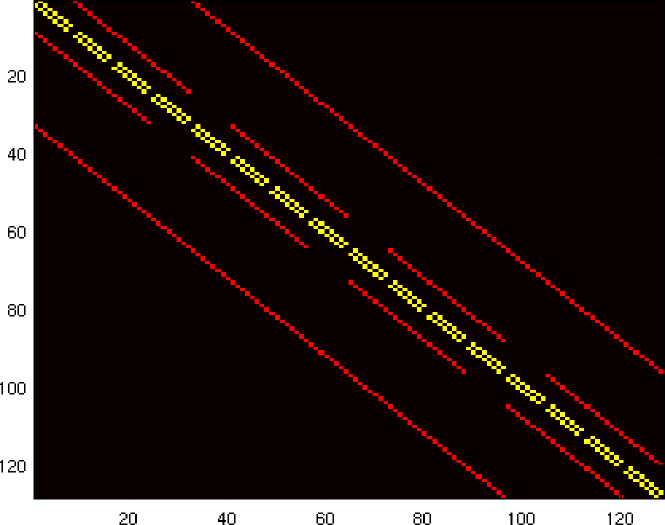
(a) Finest

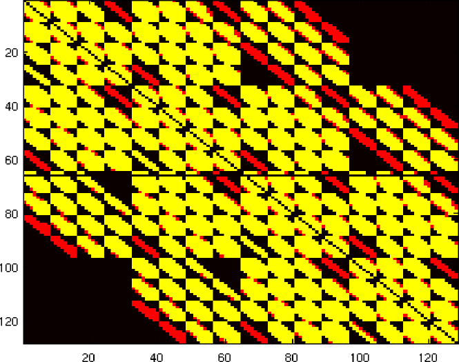
(b) Coarsest

Figure 1: Communication patterns for MueLu at different hierarchy levels (no repartitioning).

IV Fault Model and Injection Methodology

This work is motivated by the premise that soft errors will become more likely in future systems, and that SDC has been observed in current systems. Much uncertainty remains about how how often soft errors will occur, and how they will manifest in applications. Most prior work modeled soft errors as one or more flipped bits e.g., [25]. Researchers injected bit flips and observed their effects on running applications [26, 9, 27]. These works showed that current algorithms can misbehave badly if their data are corrupted. In the presence of SDC, iterative methods can either return the wrong answer, or fail to converge and iterate forever. What previous results have not achieved, though, is to give algorithm designers tools to prove that one algorithm is better than another algorithm.

For this reason, we intentionally choose a fault model that is abstract. Regardless of how a soft error occurs, we do know that if the soft error creates SDC, then we can represent the SDC as a numerical error in our algorithm. We make neither a claim to address all problems that soft errors may introduce, nor do we specifically focus on the event that incorrect data are used in a calculation. This enables our work to address a larger set of errors than the bit flip model does, e.g., corruption of a network packet. Since our results show what happens if an entire MPI process returns tainted data, they may also guide development of alternatives to C/R recovery that replace data from a lost process with a best guess.

We intentionally avoid injecting faults at a high rate, because it is not clear that soft error rates will be high. Vendors have strong incentives to sell reliable machines, at least at small scales of parallelism, but may accept that the largest-scale parallel machines might expose some faults to applications. Alternately, some systems might provide less reliable “stochastic circuits” as low-power or high-performance accelerators, to which users may allocate portions of their computation. Our model covers all of these cases.

IV-A Modeling “Bad” Faults in Preconditioners

Since we do not know the answers to many questions regarding soft errors in future systems, we choose to create errors that we know are “very bad” and observe how our algorithms handle these egregious errors. We define “bad” errors in the next paragraph, but the idea is for such errors to have meaningful effects on the solver. We denote the vector output of a preconditioner as $z$ (see, e.g., Line 18 of Algorithm 2). In numerical analysis, we describe errors using norms. GMRES minimizes the residual error with respect to the L-2 norm, and CG minimizes the $A$-norm of the solution error, which is also an L-2 norm of a different vector. For this reason, we choose to characterize errors with respect to the L-2 norm. This leads us to two classifications of errors: Those that change the L-2 norm of the output, and those that preserve its L-2 norm.

We define a bad error to be a faulty subdomain permuting its portion of the global vector. Permutations preserve the L-2 norm. We also consider the case that this bad error changes the L-2 norm. To change the L-2 norm, a faulty subdomain may also scale its portion of the vector by some constant (faulty domains always permute). Scaling a portion of the global (distributed) vector might not change the L-2 norm by that amount globally, since only a portion of the vector is scaled. Should we fault all ranks, then we see in that case that the global vector’s length is changed by some factor.

IV-B Granularity of Faults

In our fault model, we let subdomains (one subdomain per MPI process) return completely corrupt solutions. That is, we consider faults at the MPI process level, rather than single values. This seems pessimistic, but it lets us model faults inside a preconditioner that may affect more than one entry of its output vector, and possibly even more than one process. For example, an incorrect pivot in a sparse factorization for AMG’s coarse-grid solve may cause incorrect values on all processes. What our fault model promises is to characterize SDC that arises from the preconditioner in the inner solver of our fault-tolerant inner-outer iteration. We show in our results that these types of faults are sufficiently bad to cause the entire inner solve to become divergent.

IV-C SDC and Solvers

In FT-GMRES, GMRES was chosen as the inner solver because it is commonly accepted as “more robust” than CG. Given that CG can only solve SPD linear systems, if a fault occurs in CG, the error can cause problems by appearing to be nonsymmetric [28], and CG can behave very poorly. It is for these reason we that CG is not considered as an outer solver. SDC may also change the sign of key values, e.g., a negative projection length. We consider sign-changing SDC by negatively scaling the output vector, which is length preserving if the scaling factor is $-1$.

V Results

V-A Methodology

We described in § IV how we corrupt the preconditioner’s output. To evaluate the impact of our preconditioned solvers in the presence of SDC, we perform the following steps:

1. Solve the problem injecting no SDC, and compute the number of times, $K$, the preconditioner was applied.

2. For all $j$ in $[1,K]$, reattempt the solve, introducing SDC at the $j$-th preconditioner application. This results in $K$ total solves.

3. For all $K$ solves with SDC, compute the relative percent of additional preconditioner applies over the SDC-free solve, e.g., $(Applies_{observed}-Applies_{FailureFree})/Applies_{FailureFree}\times 100$

4. Repeat Steps 2 and 1, letting various numbers of MPI processes participate in the SDC injection.

5. Repeat Steps 2-4, varying the scaling factor applied to the SDC.

6. For each combination of scaling factor and number of faulty processes, plot the average number of additional preconditioner applies as a percentage. 0% means no additional applies; 100% means twice as many.

V-B Strong Scaling

We present two studies. First, we fix the problem size and strongly scale by increasing the number of MPI processes. We start with 32 processes, and then use 1032 processes on the NERSC Hopper cluster. We choose 5 fixed numbers of faulty ranks: 1, 2, 8, 16, and 32. By strong scaling the problem, the percentage of work per process decreases. Hence, the percent of the global output vector that is tainted by SDC decreases.

V-C Weak Scaling

Second, we weak scale a problem such that the work per process remains fixed at $10^{5}$ unknowns. In this experiment, we consider faults as a percentage, rather than a fixed number, of the process count. This decision is based on the fact that strong scaling demonstrates how increasing the process count minimizes the amount of corruption a single process can introduce. With weak scaling, the global problem size must increase sufficiently to minimize the impact of a single process faulting. Also, multilevel preconditioners communicate information at different grid levels. A fault at the coarsest grid could propagate, tainting data on all nodes by the time the finest grid is reached. Thus, it makes sense for multigrid to explore a percentage of ranks faulting. 100% of ranks faulting is akin to a drastic fault at the coarsest level that corrupts everything. 50% of ranks faulting would be a drastic fault at the 2^nd coarsest level of the hierarchy.

V-D Test Problems

We evaluate two classes of problems and use solvers and preconditioners appropriate for each. We consider a SPD linear system (Poisson problem), which is solvable by both CG and GMRES. For this type of problem AMG (MueLu) represents a good preconditioner. This yields the fault tolerant solvers FGmres->Cg->MueLu and FGmres->Gmres->MueLu. We also consider a non-symmetric problem, CoupCons3D [29], which is very ill-conditioned. We may only solve CoupCons3D using GMRES, and ILU(0) is a suitable preconditioner, yielding FGmres->Gmres->ILU. We may only weak scale our Poisson problem, as it is generated, allowing us to dynamically increase the matrix size.

V-E Preconditioner Effectiveness

We intentionally chose the preconditioners evaluated. For the problems presented, MueLu represents a very good preconditioner, while ILU represents a “better than nothing” preconditioner. In terms of computational cost, MueLu is much more expensive to apply than ILU, and also requires more communication. The increased work performed by MueLu results in it solving the Poisson problem in approximately 6 total applies. Contrasted to ILU and the CoupCons3D problem, FGmres->Gmres->ILU requires 100 ILU applications. So, MueLu is expensive to apply, meaning we do not want to apply it significantly more times than necessary. Conversely, ILU is cheap to apply and additional applications are not as costly.

VI Strong Scaling Results

VI-A Incomplete LU Preconditioning

Fig. 2 shows the result of strong scaling the CoupCons3D problem from 32 to 1032 MPI processes. For the CoupCons3D problem, we require 100 preconditioner applications in a failure free environment. Consider Fig. 2(a), the y-axis represents the number of Additive Schwarz subdomains that participate in the fault. The x-axis indicates whether the SDC decreases, maintains (center column), or increases the L-2 norm of the preconditioners output. The color indicates the percent increase in preconditioner applications. The bottom row of colored squares represent rare, bad SDC. Moving vertically, we increase the number of ranks that experience a fault.

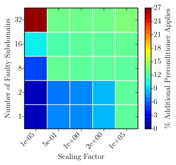
(a) 32 subdomains

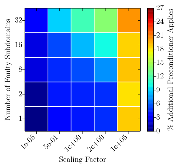
(b) 1032 subdomains

Figure 2: Strong Scaling (32 vs. 1032 subdomains): Average percent increase of preconditioner applies when solving a non-symmetric problem using FGmres->Gmres->ILU preconditioning.

In general, we see that a single faulty subdomain is tolerated with very low overhead, that is, we perform little or no additional work relative to if no fault had occurred. We also see that SDC that increases the 2-norm is universally bad, while SDC that maintains or shrinks the 2-norm is typically better than increasing the 2-norm. The exception to this is the upper left-hand block, which corresponds to 32 fault subdomains (all ranks faulted), and all ranks decreased the 2-norm by a factor of $10^{-5}$.

In Fig. 2(b), we strong scale the problem from 32 processes to 1032. We see a trend: faults that corrupt, while preserving or shrinking the 2-norm have considerably lower overhead than faults that increase the 2-norm.

We can conclude from this experiment that our Selective Reliability scheme offers dynamic fault tolerance. That is, when faults are rare, we perform less fault tolerance work, and when faults are more common we automatically perform more work without the need to explicitly detect and correct any errors. This dynamic approach is enabled by coupling systems fault tolerance and numerical analysis.

VI-B Algebraic Multigrid Preconditioning

Next, we consider solving the SPD Poisson problem. This problem is suitable for CG or GMRES, and MueLu is a very effective preconditioner. The effectiveness of MueLu as a preconditioner means that we apply it a very small number of times: We require 6 preconditioner applications in a failure free environment.

Fig. 3 shows the average percentage of additional MueLu applies given Fgmres->Cg->MueLu as the solver. It is immediately clear that there is a trend (see Fig. 2), where length preserving or shrinking faults incur lower overhead than length increasing SDC. Starting in the lower left-hand corner of Fig. 3(a), we see that SDC induced very little additional work (typically 0 or 1 additional MueLu apply). Moving towards the right, we observe that SDC slightly shrinks the L-2 norm of the preconditioner output. Again, we see a low overhead. As we continue to move towards the lower right-hand corner, we observe that SDCs introduce large overhead. These faults correspond to length (L-2 norm) increasing SDC. If we start in the lower left-hand corner and move vertically, we increase the number of subdomains that participate in the SDC. Given a single faulty subdomain (MPI rank), we observe that the overhead introduced by SDC is lower, and as the number of faulty subdomains increases, the overhead from SDC increases. This result is expected, since increasing the number of faulty subdomains increases the amount of corruption introduced into the calculations. And because we have strongly scaled the experiments, this also means we have increased the percentage of corruption. For the 32 subdomain run (Fig. 3(a)), the top row shows that every rank faulted.

We now observe the same trend as above, in the 1032 subdomain job. Starting in the lower left-hand corner and moving towards the right, we see very low overhead until we encounter an SDC that increases the L-2 norm (bottom right-most two squares). Here, SDC caused slightly more overhead for a small increase in the L-2 norm, and very high overhead for a large increase (the bottom right-most square). Moving vertically from the lower left-hand corner, we observe an SDC that shrinks the L-2 norm also provides the lowest overhead. When moving towards the right, the overhead increases.

We further observe a 3.2x increase in preconditioner calls in the worst case when 32 processors are used. But when strongly scaled to 1032 processors, we see that length preserving or decreasing faults incur relatively low overhead, e.g., a 0-40% increase in preconditioner calls (0-3 additional applies).

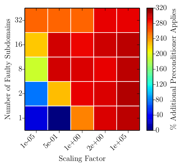
(a) 32 subdomains

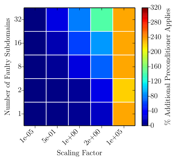
(b) 1032 subdomains

Figure 3: Strong Scaling (32 vs. 1032 subdomains): Average percent increase of preconditioner applies when solving a symmetric positive definite problem using FGmres->Cg->MueLu preconditioning.

Fig. 4 depicts results from FGmres->Gmres->MueLu to solve the SPD problem. We see the same trend as described in the FGmres->Cg->MueLu case. The lower left-hand corner represents the lowest overhead, and moving vertically or horizontally from this quadrant increases the overhead introduced by SDC. This trend is shown in both the 32 subdomain and 1032 subdomain runs.

It is immediately clear that FGmres->Cg->MueLu is superior in terms of overhead at both 32 and 1032 processes. The worst case for GMRES is a 500% increase versus CG’s 320%. We believe the cause for this is due to GMRES preserving state (having “memory”), while CG is mostly stateless. A fault in GMRES is embedded into the subspace that is built, where as CG is effectively a 3-term recurrence. This gives CG as an inner solver a chance to recover without wasting an entire inner solve. GMRES appears to have difficulty recovering from corruption to its basis. We leave further analysis to future work but recommend FGmres->Cg for SPD problems with a good preconditioner. We next consider some detection strategies, i.e., if you are using an expensive preconditioner, it may pay off to check the explicit residual.

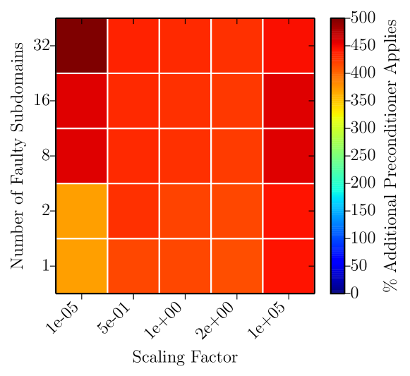
(a) 32 subdomains

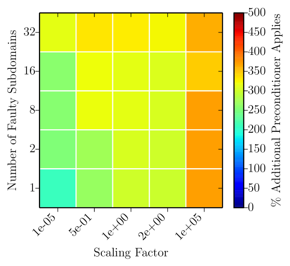
(b) 1032 subdomains

Figure 4: Strong Scaling (32 vs. 1032 subdomains): Average percent increase of preconditioner applies when solving a symmetric positive definite problem using FGmres->Gmres->MueLu preconditioning.

VI-C Optional Detection Strategies

Faults in inner solves are silent. Our solvers must either converge through them or detect them and possibly roll back a failed inner solve. Detection cannot catch all SDC, and it also does not even need to, particularly for small errors. We discussed a trend in our results showing that SDCs that shrink or maintain the L-2 norm of the preconditioner’s output are optimal with respect to SDC that increases the L-2 norm. Nonetheless, detection may help avoid wasted work in a failed inner solve. In the previous section’s results, we did not attempt to detect SDC or roll back iterations in inner solves. With an expensive but effective preconditioner, failed inner solves may have high overhead.

In this section, we evaluate two different error detectors by observing whether they would have triggered given the faults presented. We saw in the last section (compare Figures 3 and 4) that GMRES as an inner solver has less resilience to faults than CG for SPD problems. However, GMRES has a built-in invariant that CG lacks, namely that the 2-norm of the explicitly computed residual $r_{k}=b-Ax_{k}$ will never increase. Both CG and GMRES can use projection length bounds on intermediate basis vectors to detect faults, but only GMRES can use the monotonicity of $\|r_{k}\|_{2}$. We now consider if detection strategies in GMRES make sense relative to CG’s relatively lower fault tolerance overhead.

VI-D Detection Strategies: Non-Symmetric Problem

We use the data from Fig. 2(a) to create Fig. 5(a). We have superimposed ’\’ to indicate that the explicit residual detected the error, and ’$/$’ to indicate whether a projection length norm bound proposed by Elliott et al. [14] would be triggered. We see that the explicit residual caught all SDCs introduced, while the projection length bound only caught errors that drastically increased the 2-norm of the preconditioner’s output. The norm bound proves extremely effective, given its cheapness to evaluate relative to the cost of computing the explicit residual.

Fig. 5(b) shows the effect of responding to these checks. We see at most $2=100\times.018$ extra preconditioner applications. Recall that CoupCons3D with GMRES required 100 preconditioner applications with no faults. Given the cost of computing the explicit residual, relative to the cost of applying ILU, it is not clear that checking the explicit residual every iteration is worth the overhead. We found experimentally that checking the explicit residual every 5 iterations sufficed (data omitted due to space).

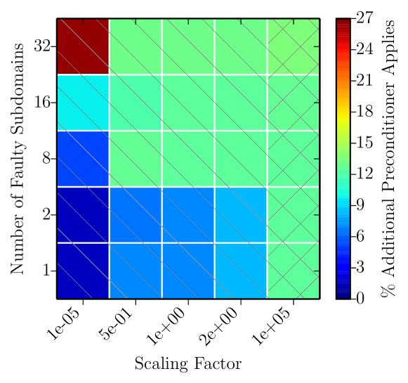
(a) Faults that could be detected by the norm bound presented in [14] are hatched right $/$, and faults that could be detected by checking the explicit residual are hatched left \.

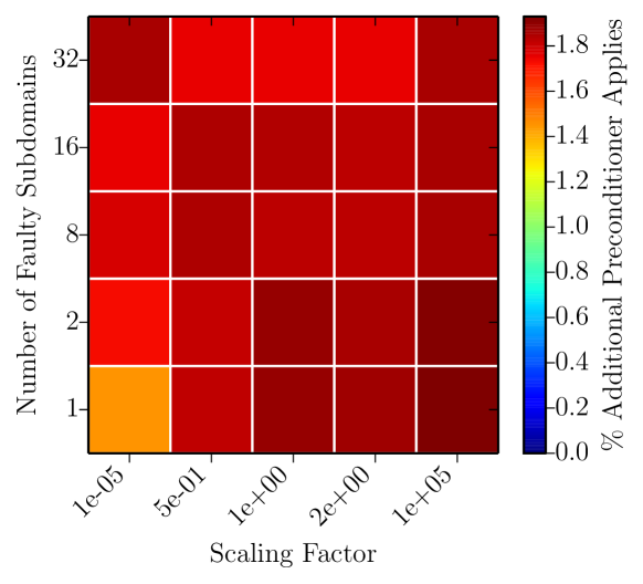
(b) Responding to norm bound or explicit residual check to exit inner solve early (note the colorbar range is different).

Figure 5: Strong Scaling: Average percent increase of preconditioner applies when solving a non-symmetric problem using FGmres->Gmres->ILU preconditioning, and checking projection lengths and explicit residuals every iteration. These plots uses 32 subdomains (MPI ranks).

VI-E Detection Strategies: Symmetric Problem

Fig. 6 takes the data from Fig. 4(a) and superimposes the detectors. Recall that GMRES had very poor behavior compared to CG in this case. We see that the norm bound by Elliott et al. [14] has good coverage for the Poisson problem. This is due to the spectral norm of A being relatively small compared to the CoupCons3D spectral norm (which has order $10^{+6}$). We see that by using detectors, we can make GMRES’s fault tolerance overhead much smaller than CG: 120% (GMRES) vs 320% (CG). Seven extra preconditioner calls are required for GMRES and 20 for CG. Given the cost of applying MueLu, it pays to use GMRES and then to compute the explicit residual.

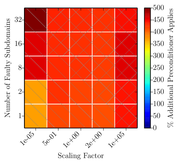
(a) Faults that could be detected by the norm bound presented in [14] are hatched right $/$, and faults that could be detected by checking the explicit residual are hatched left \.

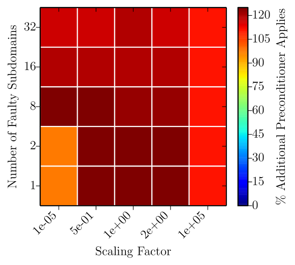
(b) Responding to norm bound or explicit residual check to exit inner solve early (note the colorbar range is different).

Figure 6: Strong Scaling: Average percent increase of preconditioner applies when solving an SPD problem using FGmres->Gmres->MueLu preconditioning, and checking projection lengths and explicit residuals every iteration. These plots uses 32 subdomains (MPI ranks).

We now take into account the cost of a GMRES iteration vs a CG iteration. GMRES’s work grows linearly with the number of iterations it performs. We consider work to be the number of dot products per iteration, since sparse matrix-vector multiplication (SpMVs) are the same for CG and GMRES. Given that GMRES needs a total of $6+7$ inner iterations to converge (one preconditioner apply per inner iteration) and CG required $6+20$ inner iterations, the dot products for GMRES are $(13\times 14)/2=91$, while CG requires $26\times 2=52$.

We now account for the preconditioner applications. Right preconditioned GMRES requires a preconditioner application to compute the explicit residual, meaning that if the explicit residual was checked every iteration, then 13 inner iterations would require $13\times 2=26$ preconditioner applies. Left preconditioned CG requires no preconditioner applications to compute the explicit residual, and, hence, just 26 preconditioner applications suffice.

In summary, with detectors, GMRES required $91$ dot products and $26$ preconditioner applications, while CG required $52$ dot products and $26$ preconditioner applications. These findings still favor CG as the inner solver. The norm bound from Elliott et al. [14] flagged 50% of the errors, meaning no explicit residual check would be required. We found experimentally that checking the explicit residual every 5 iterations was sufficient for lowering the overhead in GMRES. Taking this into account, we can slightly reduce the number of preconditioner applies required, but also incur more dot products (as we can iterate up to 5 iterations before detecting that a fault occurred).

This is a surprising result. GMRES + detectors beats CG, but the overhead of computing the detectors allows CG to win. If the preconditioner is sufficiently expensive to apply, then it makes sense to use GMRES + detectors, since it can detect and rollback the inner solve should an error occur. CG does not support the explicit residual check, as it does not promise a non-increasing residual. We leave to future work incorporating the norm bound check into CG. With a projection length check, we expect CG to be a clear winner over GMRES.

VI-E1 FGMRES as the Inner Solver

The premise behind Selective Reliability and nesting solvers is that users who are not experts in numerical algorithms can take existing solver / preconditioner combinations and easily nest them inside a reliable Flexible GMRES outer solver. This enables a “black box” approach to iterative solver reliability. If we also choose the inner solver to yield the lowest fault tolerance overhead, then we should consider all solvers, including Flexible GMRES, as the inner solver, e.g., FGmres->FGmres->MueLu. Fig. 7 presents this case. We see that if we trade memory (Flexible GMRES requires storing two sets of basis vectors), then we obtain significantly lower fault tolerance overhead. Also, FGMRES does not require the application of the preconditioner to compute the explicit residual, meaning that explicit residual checks are inexpensive even if the preconditioner is very expensive.

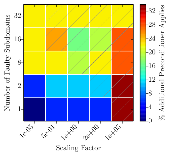
Figure 7: Faults that could be detected by the norm bound presented in [14] are hatched right $/$, and faults that could be detected by checking the explicit residual are hatched left \, when solving an SPD problem using FGmres->FGmres->MueLu. This plot uses a total of 32 subdomains (MPI ranks).

VI-E2 Robustness of Projection Length

An unexpected result is shown in Fig. 6(a). The projection length check flags SDC where the L-2 norm of the preconditioner output preserves, increase, or decreases. In this case, the norm bound from Elliott [14] is approximately $3.6\times 10^{2}$, which is relatively tight. The projection length bound is not checked immediately after calling the preconditioner, but is instead checked as the upper Hessenberg is formed, e.g., in Line 18 of Algorithm 1. In Fig. 8 we show what is detectable when then problem is strongly scaled, e.g., Fig. 4 with detectors overlaid. We see that the explicit residual failed to detect any errors, yet the norm bound still succeeded in detecting the most costly errors.

Figure 8: Strong Scaling: Faults that could be detected by the norm bound presented in [14] are hatched right $/$, and faults that could be detected by checking the explicit residual are hatched left \, when solving an SPD problem using FGmres->Gmres->MueLu. This plot uses a total of 1032 subdomains (MPI ranks) and should be compared to Fig. 5(a) .

VI-F Impact of Sign Changes

We now consider the impact of a sign-changing fault with CG. CG can behave badly if its step length ($\alpha$ in Alg. 2) is incorrect. Figure 9 shows the results of solving the Poisson problem using FGmres->Cg->MueLu, with both positive and negative SDC scaling factors. We see that the errors we deem “bad”, i.e., permuting and scaling, are large. For GMRES, the figure is a symmetric version of Fig. 4(a) (omitted due to space).

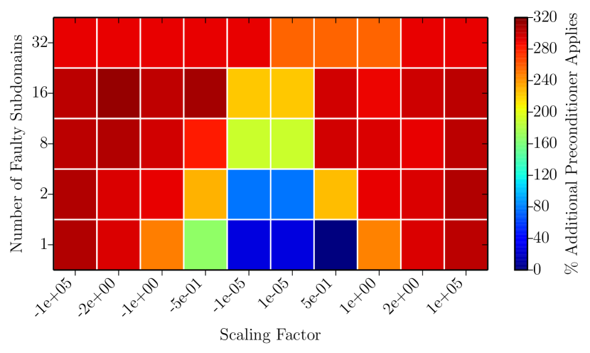
Figure 9: Strong Scaling: Average number of additional preconditioner applies given faults that change the sign of the preconditioner output when solving with FGmres->Cg->MueLu. This plot uses 32 subdomains (MPI processes).

VII Weak Scaling Results

We now take the Poisson problem and fix the work per processor to 100k unknowns. We then weakly scale the problem to 24 process (one node) and 1032 processes (43 nodes) on the NERSC Hopper cluster. This yields a global matrix size of approximately 102.3 million and required approximately 1TB of memory.

Fig. 10 shows that the problem size has a clear impact on fault tolerance. Should an error taint every subdomain, e.g., from interpolations from a coarse grid, then we see nearly a 100% different in fault tolerance overhead between the worst SDC in the smaller problem (Fig. 10(a)) and the larger problem (Fig. 10(b)). We also see the repeated trend that faults that maintain and do not drastically increase the 2-norm of the preconditioner output typically incur lower fault tolerance overhead. Note: The bottom row of squares (4% and 0% Faulty Subdomains) correspond to a single process creating SDC.

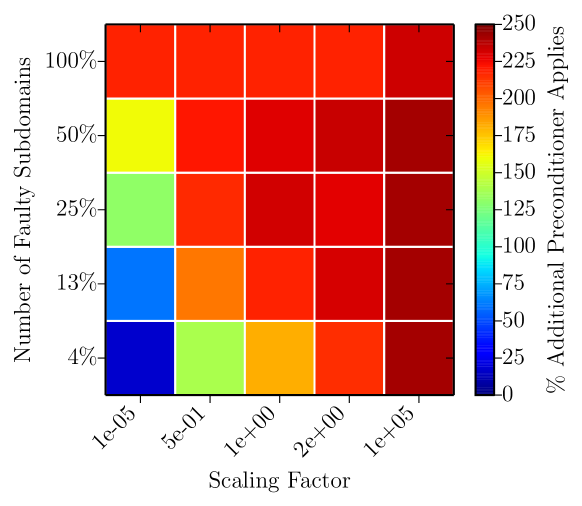
(a) 24 subdomains with 100k unknowns per process.

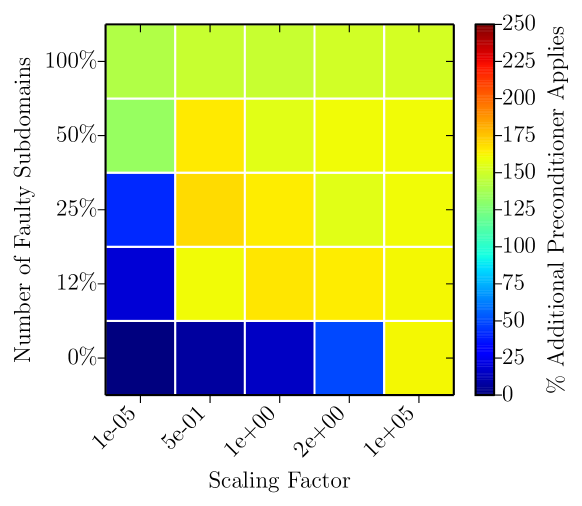
(b) 1032 subdomains with 100k unknowns per process.

Figure 10: Weak Scaling (24 vs. 1032 subdomains): Average percent increase of preconditioner applies when solving an SPD problem using FGmres->Cg->MueLu preconditioning weak scaled to 24 processors and 1032 processors

VIII Conclusion

This paper demonstrates that iterative linear solvers can get the right answer despite incorrect arithmetic or storage in their preconditioners. They can do so without algorithmic or implementation changes to preconditioners by combining selective reliability and inner-outer iterations. Fault detection in inner solves need not catch all incorrect preconditioner results in order to reduce overhead much below just running the solver twice. This justifies even an expensive implementation of reliability in outer solves, since most of the work goes into inner solves with their more effective preconditioner. We have also shown that analytical approaches that detect and filter out large errors scale well and significantly reduce faults’ overhead. This is particularly true for effective preconditioners like algebraic multigrid, that require only a few solver iterations, but whose complexity and global communication patterns may make them more vulnerable to SDC. Combining the projection norm bound from Elliott [14] with an occasional check for monotonicity of the explicit residual norm in GMRES detected more faults than either alone.

We have presented results based on a fault model that is possible given future soft fault projections. Given what little we know about how faults will appear in future hardware, we have chosen to use faults that represent an entire MPI process returning incorrect data. Our fault model does not aim to predict actual behavior of future SDC. Rather, it shows a case sufficiently “bad” for us to assess how our fault tolerance strategies behave when presented with very damaging SDC.

Whether SDC turns out to be a real “monster in the closet” or not, our findings are relevant for other fields of research. We observe a consistent trend in our data: Faults that increase the 2-norm are worse than faults that maintain or decrease the 2-norm. We also see that when the number of faulty ranks is low, returning data that is wrong but “small” (in the L-2 norm sense) is optimal. This suggests a strategy for dealing with failure of MPI processes or other data loss, namely, replacing the missing data with “small” values and continuing the solve. Future work will pursue with our collaborators this common strategy for recovery from both soft and hard faults. We also plan to compare the performance of this paper’s approach with that of software checksums and other resilience techniques. Finally, we will investigate the development and use of programming models that provide selective reliability.

References

- [1] S. Michalak, A. Dubois, C. Storlie, H. Quinn, W. Rust, D. DuBois, D. Modl, A. Manuzzato, and S. Blanchard, “Assessment of the impact of cosmic-ray-induced neutrons on hardware in the Roadrunner supercomputer,” Device and Materials Reliability, IEEE Transactions on, vol. 12, no. 2, pp. 445–454, 2012.
- [2] P. Kogge et al., “ExaScale computing study: Technology challenges in achieving exascale systems,” Defense Advanced Research Project Agency, Information Processing Techniques Office, Tech. Rep., 2008. [Online]. Available: http://users.ece.gatech.edu/mrichard/ExascaleComputingStudyReports/exascale_final_report_100208.pdf
- [3] A. Geist, “What is the monster in the closet?” Aug. 2011, invited Talk at Workshop on Architectures I: Exascale and Beyond: Gaps in Research, Gaps in our Thinking.
- [4] A. Moody, G. Bronevetsky, K. Mohror, and B. de Supinski, “Design, modeling, and evaluation of a scalable multi-level checkpointing system,” in Supercomputing, Nov. 2010.
- [5] Z. Chen, “Algorithm-based recovery for iterative methods without checkpointing,” in Symposium on High-Performance Parallel and Distributed Computing, Jun. 2011, pp. 73–84.
- [6] J. Schlaich and K.-H. Raineck, “Die Ursache für den Totalverlust der Betonplattform Sleipner A,” Beton- und Stahlbetonbau, vol. 88, pp. 1–4, 1993.
- [7] J. Gaidamour, J. Hu, C. Siefert, and R. Tuminaro, “Design considerations for a flexible multigrid preconditioning library,” Scientific Programming, vol. 20, no. 3, pp. 223–239, 2012.
- [8] T. Davies, C. Karlsson, H. Liu, C. Ding, and Z. Chen, “High performance LINPACK benchmark: A fault tolerant implementation without checkpointing,” in Proceedings of the 25th Annual International Conference on Supercomputing, May 2011, pp. 162–171.
- [9] T. Davies and Z. Chen, “Correcting soft errors online in LU factorization,” in Proceedings of the 22nd International Symposium on High-Performance Parallel and Distributed Computing, ser. HPDC ’13. New York, NY, USA: ACM, 2013, pp. 167–178.
- [10] Y. Chen and Y. Deng, “A detailed analysis of communication load balance on bluegene supercomputer,” Comp. Phys. Comm., vol. 180, no. 8, pp. 1251–1258, 2009.
- [11] K.-H. Huang and J. A. Abraham, “Algorithm-based fault tolerance for matrix operations,” IEEE Transactions on Computers, vol. C-33, no. 6, pp. 518–528, Jun. 1984.
- [12] M. Shantharam, S. Srinivasmurthy, and P. Raghavan, “Fault tolerant preconditioned conjugate gradient for sparse linear system solution,” in Proceedings of the 26th ACM International Conference on Supercomputing, ser. ICS ’12. New York, NY, USA: ACM, 2012, pp. 69–78.
- [13] P. G. Bridges, K. B. Ferreira, M. A. Heroux, and M. Hoemmen, “Fault-tolerant linear solvers via selective reliability,” ArXiv e-prints, Jun. 2012, provided by the SAO/NASA Astrophysics Data System.
- [14] J. Elliott, M. Hoemmen, and F. Mueller, “Evaluating the impact of SDC on the GMRES iterative solver,” in 28th IEEE International Parallel & Distributed Processing Symposium (IEEE IPDPS 2014), Phoenix, USA, May 2014.
- [15] Y. Saad and M. H. Schultz, “GMRES: A generalized minimal residual algorithm for solving nonsymmetric linear systems,” SIAM J. Sci. Stat. Comput., vol. 7, no. 3, pp. 856–869, Jul. 1986.
- [16] M. R. Hestenes and E. Stiefel, “Methods of Conjugate Gradients for Solving Linear Systems,” Journal of Research of the National Bureau of Standards, vol. 49, no. 6, pp. 409–436, Dec. 1952.
- [17] D. H. Bailey, E. Barszcz, J. T. Barton, D. S. Browning, R. L. Carter, D. Dagum, R. A. Fatoohi, P. O. Frederickson, T. A. Lasinski, R. S. Schreiber, H. D. Simon, V. Venkatakrishnan, and S. K. Weeratunga, “The NAS Parallel Benchmarks,” The International Journal of Supercomputer Applications, vol. 5, no. 3, pp. 63–73, Fall 1991. [Online]. Available: citeseer.ist.psu.edu/article/bailey94nas.html
- [18] M. A. Heroux et al., “Improving performance via mini-applications,” Sandia National Laboratories, Tech. Rep. SAND2009-5574, September 2009.
- [19] Y. Saad, Iterative Methods for Sparse Linear Systems, 2nd ed. Philadelphia, PA, USA: Society for Industrial and Applied Mathematics, 2003.
- [20] C. G. Baker and M. A. Heroux, “Tpetra, and the use of generic programming in scientific computing,” Scientific Programming, vol. 20, no. 2, pp. 115–128, 2012.
- [21] M. Heroux, R. Bartlett, V. H. R. Hoekstra, J. Hu, T. Kolda, R. Lehoucq, K. Long, R. Pawlowski, E. Phipps, A. Salinger, H. Thornquist, R. Tuminaro, J. Willenbring, and A. Williams, “An Overview of Trilinos,” Sandia National Laboratories, Tech. Rep. SAND2003-2927, 2003.
- [22] E. Bavier, M. Hoemmen, S. Rajamanickam, and H. Thornquist, “Amesos2 and Belos: Direct and iterative solvers for large sparse linear systems,” Scientific Programming, vol. 20, no. 3, pp. 241–255, 2012.
- [23] B. F. Smith, P. E. Bjørstad, and W. D. Gropp, Domain Decomposition: Parallel Multilevel Methods for Elliptic Partial Differential Equations. New York: Cambridge University Press, 1996.
- [24] J. W. Demmel, S. C. Eisenstat, J. R. Gilbert, X. S. Li, and J. W. H. Liu, “A supernodal approach to sparse partial pivoting,” SIAM J. Matrix Analysis and Applications, vol. 20, no. 3, pp. 720–755, 1999.
- [25] J. Sloan, R. Kumar, and G. Bronevetsky, “Algorithmic approaches to low overhead fault detection for sparse linear algebra,” in Proceedings of the 2012 42nd Annual IEEE/IFIP International Conference on Dependable Systems and Networks (DSN), ser. DSN ’12. Washington, DC, USA: IEEE Computer Society, 2012, pp. 1–12. [Online]. Available: http://dl.acm.org/citation.cfm?id=2354410.2355166
- [26] M. Shantharam, S. Srinivasmurthy, and P. Raghavan, “Characterizing the impact of soft errors on iterative methods in scientific computing,” in Proceedings of the 25th International Conference on Supercomputing, ser. ICS ’11. New York, NY, USA: ACM, 2011, pp. 152–161.
- [27] P. Sao and R. Vuduc, “Self-stabilizing iterative solvers,” in Proceedings of the Workshop on Latest Advances in Scalable Algorithms for Large-Scale Systems, ser. ScalA ’13. New York, NY, USA: ACM, 2013, pp. 4:1–4:8.
- [28] A. Meek, V. Howle, and M. Hoemmen, “Fault Tolerant QMR,” Minisymposium talk at SIAM Computational Science and Engineering, Feb. 2013.
- [29] T. A. Davis and Y. Hu, “The University of Florida Sparse Matrix Collection,” ACM Transactions on Mathematical Software, vol. 38, no. 1, pp. 1:1–1:25, 2011.